Georeferencing Historical Maps at Scale

Abstract
This paper presents a novel approach to automatically georeferencing historical maps using an algorithm based on salient line intersections. Our algorithm addresses the challenges inherent in linking historical map images to contemporary cadastral data, particularly those due to temporal discrepancies, cartographic distortions, and map image noise. By extracting and comparing angular relationships between cadastral features, termed monads and dyads, we establish a robust method for performing record linkage by identifying corresponding spatial patterns across disparate datasets. We employ a Bayesian framework to quantify the likelihood of dyad matches corrupted by measurement noise. The algorithm’s performance was evaluated by selecting a map image and finding putative angle correspondences from the entirety of Aotearoa New Zealand. Even when restricted to a single dyad match, >99% of candidate regions can be successfully filtered out. We discuss the implications and limitations, and suggest strategies for further enhancing the algorithm’s robustness and efficiency. Our work is motivated by previous work in the areas of critical GIS, critical cartography and spatial justice and seeks to contribute to the areas of Spatial Data Science, Historical GIS and GIScience.
Keywords and phrases:
Historical GIS, Georeferencing, Record Linkage, Spatial Data JusticeCopyright and License:
2012 ACM Subject Classification:
Applied computing Mathematics and statistics ; Applied computing Earth and atmospheric sciences ; Applied computing Arts and humanitiesAcknowledgements:
Kei ngā mātāpuputu, ko David te puna mōhio, ko Sydney Shep te kanohi hōmiromiro, ko Rhys Owen te reo pono, kei ngā hoa, kei ngā whānau, tēnā koutou katoa.Editors:
Katarzyna Sila-Nowicka, Antoni Moore, David O'Sullivan, Benjamin Adams, and Mark GaheganSeries and Publisher:
1 Context
Introduction
Historical maps are a cartographic record of where a place was and perhaps still is. They offer a window into the past that can support indigenous communities to reconnect with their histories, language and places. Specifically, historical cadastral maps provide a record of the evolution of land interests during the colonisation of Aotearoa New Zealand in the 19th and 20th centuries. Given that georeferencing is typically a manual and time-intensive task, these rich resources are often inaccessible to most except for those who are familiar with cartography or the local histories of the places that were mapped. By labelling points in the map and calculating their real world coordinates, georeferencing enables a broader level of accessibility to the map image and the histories embedded therein. We propose an algorithm Koki Tauriterite (translated simply as determining angle equality) that leverages the ease of detecting intersecting lines in the map image and digital cadaster to perform robust record linkage between the two sources for the purposes of large scale automatic georeferencing of historical maps in Aotearoa New Zealand.
De-colonial inspirations
For New Zealand Māori, historical maps allow one to locate traditional places of food gathering, villages and burial grounds that are no longer visible in today’s landscape due to successive generations of te muru me te raupatu (land confiscation and dispossession), where historical and contextual knowledge of said places generally exists in the minds of a few [4]. Therefore historical maps enable one to do what most cannot; locate these cultural sights of significance in space. Attempts to revitalise and make accessible this knowledge are visible around the country and the utilisation of computational tools are aiding in that process of revival, for example Ngāi Tahu’s community generated atlas tool Kā Huru Manu [11].
The processes that lead to the creation of the map in the Aotearoa New Zealand context represent a traumatic colonial history for Māori communities [4]. Power structures in the colony which sought to benefit the colonising power were perpetuated while simultaneously assimilating indigenous relationality to place via the creation of the map [12]. The role that maps played in the dispossession of Māori and their resources through the Native Land Court and other various mechanisms of the state [6] highlights a contradiction evident with the elevation of the map as an important archival record of Māori language and geographic history [5], particularly (for one of us) as a descendant of Parihaka ploughmen who were imprisoned without trial and forced into hard labour for ploughing their own confiscated land [14].
However, those same symbols of paternalistic control can also play an important role in the retrieval, preservation and eventual dissemination of Māori relationality and re-connection with place, and subsequently aid in helping to make visible that rich history to the communities from which those places belong and vise versa. Therefore, the rematriation [10] of historical maps as records of place, via the provision of wider, open access to them for indigenous communities represents a form of spatial data justice [15] that inspires and motivates this work.
2 Method
Challenges
The task amounts to record linkage between these two very different sources of data. Source 1 is a digitised image of a map – those of interest are not currently georeferenced. The state of the map and quality of digitisation is variable and, in addition, neither overall orientation nor scale can be assumed for the map since there are often scarce metadata records to accompany the map. This necessitates an approach that is therefore scale and rotation invariant. Source 2 is essentially a large list of polygons and associated geospatial information, henceforth “the cadaster”. The task of georeferencing a map amounts to finding plausible corresponding locations for an individual map, within the (large) cadaster. However the two sources use completely different representations in their raw data (images, and polygons respectively). Contrast this with astrometry for example, where both image and stellar catalogue naturally result in lists of 2d vectors which are able to be compared [13]. An effective solution will involve making a defensible correspondence between features identifiable in both map images and the cadaster.
Record linkage of cadastral data and historical map images presents a significant challenge due to inherent discrepancies between analogue and digital-borne data [16]. While both sources purportedly depict the same geographic area, they capture it at different points in time, resulting in variations in geometry present in both the survey record and the map image. Temporal changes in land use as well as cartographic conventions complicate the process of establishing accurate correspondences between the two sources of data [17]. In Aotearoa New Zealand, the cadaster is a chronological record of land title administration that has been recorded, digitised and made public by the government agency Toitū Te Whenua Land Information New Zealand (LINZ), a process which began in the mid-1980s [19]. This is the primary dataset that contains millions of polygons that represent all current parcels in Aotearoa New Zealand [18].
Herein lies another major challenge in conducting historical record linkage. While the current survey record reflects the present-day cadastral landscape, the historical map offers a snapshot of a past configuration of land ownership. Consequently, the LINZ Parcels Dataset contains numerous parcel records that are absent from the historical map due to subsequent partitions of new parcels. Therefore, the historical map may depict parcels that no longer exist in the contemporary LINZ Parcels Dataset. These disparities necessitate a robust record linkage approach accounting for the inevitable attrition of records across the temporal divide. Record linkage in this case being the process of matching and combining records from multiple sources into a single space and then subsequently assessing whether or not they are in fact describing the same object.
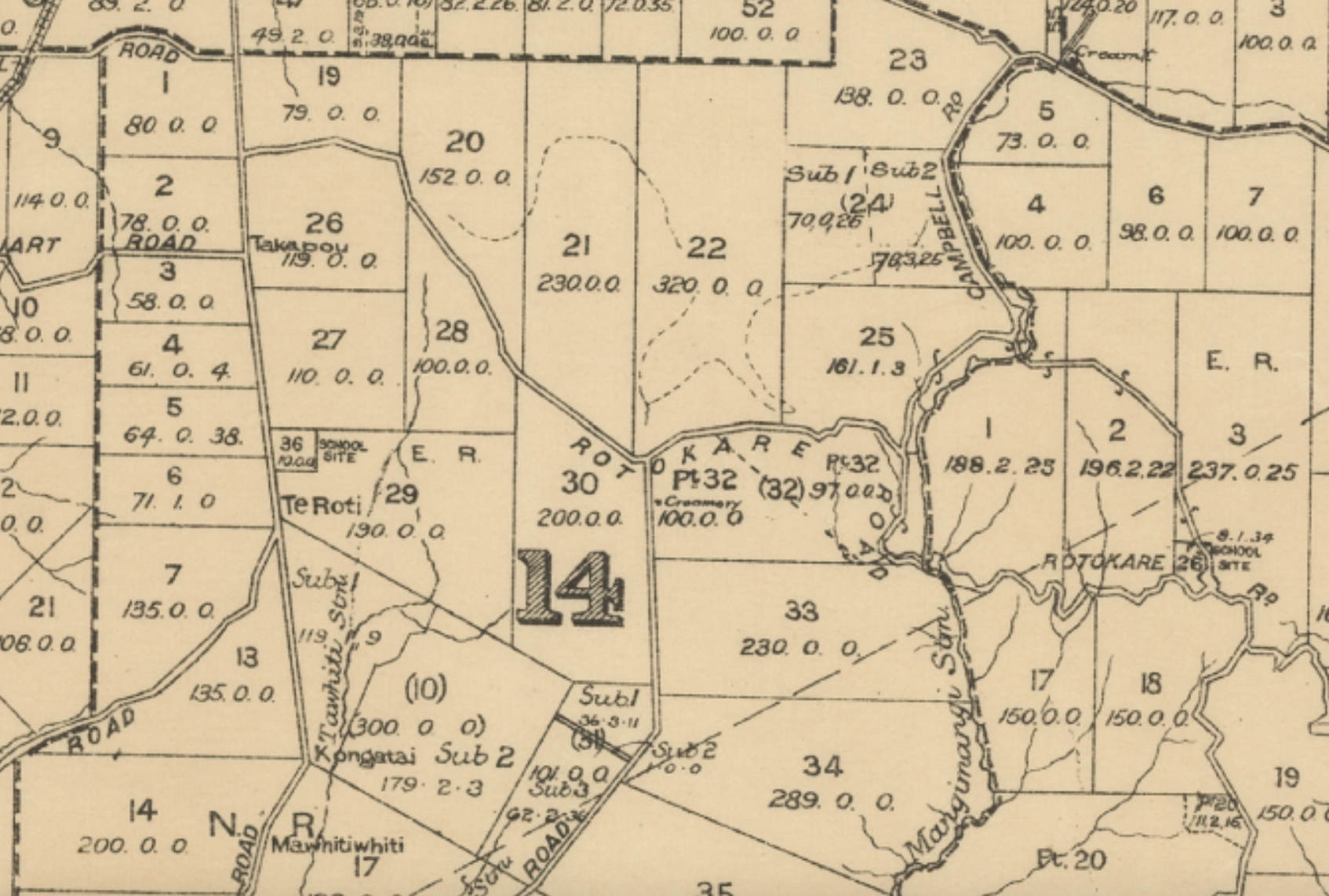
Cadastral features such as parcel boundary intersections are persistent to changes over time. Parcels of land are more often partitioned than they are amalgamated as a result of accelerated urban development in Aotearoa New Zealand during the 20th century [1]. Although the polygonal shape that is created by the parcel is generally orthogonally segmented over time, the original shape of the parcel remains identifiable in the cadaster. The original parcel may simply now have a number of lines drawn through it, for example parcel 22 in 1 is partitioned in the cadaster. These straight lines that depict parcel boundaries and the adjacent parcels they intersect with will be the basis for our analysis since there is no complete ground truth yet developed that could represent all land parcels from a particular point in time when a given map was created. Therefore a common representation space (defined below) is required to be developed upon which comparison can be performed between the two sources.

Our proposed algorithm makes use of the fact that straight lines are particularly salient in both sources (respectively via the Hough Transform [7, 3] for images and simple geometric processing for the cadaster). This supports ready identification of line intersections in either source, and characterisation by their internal angles. Agreement between sets of internal angles is useful but not diagnostic: it does not provide sufficient specificity on its own to match maps to locations. However any pair of intersections (which we call a “dyad” in what follows) furnishes another pair of angles defining their relative orientation, which provides a much more finely grained basis on which to argue for a match.
A “distance” that is low for good matches is simply the sum of squared differences in these two sets of angles, from the map and from a potential site in the cadaster:
| (1) |
Although intuitively appealing, Equation 1 requires some justification. In Section 3, we derive it from considering a Bayes factor for the probability of a match being correct, given the respective angles and , and taking careful account of their various dependencies.
Related work
In our pursuit of an effective method for georeferencing historical map images using data from the cadastral record, we explored several approaches before developing our current line intersection-based algorithm. These preliminary investigations, while ultimately not preferred, did highlight the challenges inherent in this domain. Use of image segmentation and shape recognition techniques to match full parcel polygons is one such option, but our experience has been that these methods are not robust enough to the variability inherent to historical maps, as well as the fundamental differences in spatial object representation between the cartographer’s approach and modern GIS practices that form the current cadastral record. The discrepancies in boundary delineation and feature abstraction between these two distinct technologies rendered direct shape-matching approaches unreliable. Subsequently, we explored point-based methods, employing point-finding algorithms coupled with triangulation techniques such as the Delaunay triangulation [8]. This approach, while theoretically appealing, was also found to be unsuitable, largely due to the noise present in the map images. The arbitrary addition and removal of points caused by image artifacts and inconsistencies in feature representation led to unstable and unreliable triangulations.
We also considered leveraging toponyms extracted through Optical Character Recognition (OCR) techniques in order to conduct direct georeferencing of the historical map. As is evident in Figure 2, this approach faced limitations due to the temporal disconnect between historical and contemporary place names. Many toponyms present on historical maps have since fallen into disuse or been replaced in the process of the colonisation of Aotearoa New Zealand [2]. Text on historical maps also tends to be heavily occluded, and/or follow the geography of the feature that it is describing, introducing even more complexity into the text extraction process [9]. Nevertheless, we found value in using the more persistent toponyms, such as major town names, street names or key geographic features as a means to estimate the general location of the map and thereby reduce the search space for our dyad matching pipeline (described below). These exploratory efforts underscore the complexity of the task at hand and the need for robust, noise-resistant methods in historical map analysis and record linkage.


Feature extraction
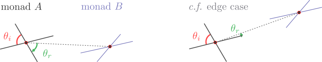
In either source, we refer to a single intersection of two straight lines as a “monad”, to contrast with “dyads” (which are pairs of intersections) that provide the main discriminating features on which our matching algorithm is based – see Figure 3 for an example. Where the intersecting line segment does not extend past another but instead generates a “T” junction, we can still treat this as an “X” shape in effect. Each monad has a characteristic angle, defined to be the smaller of the two internal angles. This is denoted if the source is the map, and if it is from the cadaster. Clearly and similarly for .
Internal angles generated by intersecting parcel boundaries are biased toward , as is evident from Figure 4. Similarly parcel boundary intersections in the cadaster result in internal angles close to , due to small line segments generated by parcels that, for instance, follow the course of a winding river or are located in urbanised areas. Furthermore, the very definition of an intersecting parcel boundary in the cadaster lends itself to complexities with respect to feature extraction since it is difficult to determine whether or not a given point in the coordinate sequence of a polygon doesn’t merely sit along a straight line. For instance in most general contexts a square shaped polygon would likely produce four unique coordinates, but in the cadaster this cannot be assumed and so two parcels could intersect along an almost straight line, producing an angle very close to . The very different nature of the two datasets (the historical map image being cartographic and the cadaster being generated computationally via survey measurements) leads to different complexities with respect to feature extraction since different methods for feature are required for the different datasets. Figure 4 confirms this very skewed distribution across the entire LINZ Parcels Dataset. The higher likelihood of seeing orthogonal or close to parallel lines reduces their discriminating power for the proposed algorithm, which relies on “suspicious coincidences” of angular relationships to attribute matches between dyad pairs.

A dyad is a set of two unique monads from the same source-this induces two further angles that are relative bearings to the line joining the monads, as illustrated in Figure 3. The range for the relative angle so defined is . Collecting these angles then, a given dyad extracted from the map image source, generated by the two monads and consists of , and similarly for a dyad extracted from the cadaster (which is a possible match for ) we have . Monads and dyads are the primary features extracted from both sources. This extraction allows for comparison to be made between the two sources thereby acting as a common representational space for matching across the sources.
Koki Tauriterite: Monad and Dyad Matching Pipeline
We first pre-filter candidate matches on the basis of monad evidence alone, in order to reduce the computational burden of matching each component part of the dyad. This reduces the search space for subsequent, more computationally intensive comparisons. The pipeline can be summarised as follows:
-
1.
Monad matching: For each monad in the map and cadaster, identify putative matches where internal angles differ by no more than degrees.
-
2.
Relative angle calculation: For each plausible pairing of monads, compute the relative bearing angles and .
-
3.
Correct for edge cases: Apply Algorithm 1 to and .
-
4.
Dyad comparison: For each candidate dyad pair, compute a similarity score based on all internal and relative angles.
-
5.
Best match selection: Select the dyad match with the lowest distance score as the most likely correspondence.
The first step filters on the angles of each monad from both sources to generate a set of putative monad-monad matches where pairs meeting the filtering condition are considered, with set to . This exclusion seeks to increase computational efficiency, although we note some potential unlikely matches are overlooked. The algorithm then calculates the relative bearing or between pairs of monads leveraging the identified putative or angle matches.
Algorithm 1 is applied at this point to relative angles, in order to correct for dramatic shifts in that can occur, should the noise present in the map image (or the cadaster) completely change the angle (or respectively). As depicted in Figure 3, this needs to be dealt with because the angle from the connecting line to the next line segment, proceeding clockwise, can either become very small or very large given only a small amount of noise. To ameliorate this fragility we check if is very close (in either direction) to the line segments that constitute the monad, or 0. If so, we generate an edge case alternative value for , referred to as , which is then later computed during the distance step alongside . The best score resulting from the comparison of these two is treated as the true . This algorithm effectively handles the edge cases for (and similarly ), adjusting based on its proximity to the edge of the monad’s line segments, while accounting for a noise factor.
Having generated putative monad matches between the two sources, the dyad selection stage can begin. This step creates the list of relative bearing angle combinations between filtered pairs of monads that each have an inter-source putative match. The algorithm then finds potential inter-source dyad matches and can therefore start to build out potential valid inter-source tuples of dyads where each constituent monad has a putative monad match that is contained in the alternative putative dyad.
The sections mentioned are those of the monad that generate the respective internal angles ( or the other, which is ), and is the line that connects the two monads to generate the relative angle . If isn’t close to either boundary it is returned unaffected.
3 Derivation of an appropriate distance for dyads
Here we derive Equation 1 from the standpoint of a generative model of dyads. Despite the apparent simplicity of the end result, care is needed as the relative angles are conditioned on the internal ones.
Suppose we have a single dyad from the map image source, characterised by angles , and a single dyad from the cadaster, characterised by angles . In addition, we have a putative association between the constituent monads delivered by the pre-processing stage: where are monads from a map and are from the cadaster. Taking the logarithm of the Bayes Factor (i.e., the ratio of probabilities for and against a match) yields a natural score, which quantifies the relative evidence in favour of a match on a logarithmic scale. Ignoring the prior degree of belief in a match (which just adds a constant anyway), we have a score for a match between dyads that is the log of a likelihood ratio:
| where “same” and “diff” refer to ground truth: the two pairs are in fact the same locations, as asserted, or are not. Using the product rule, this is | ||||
| which factors into an and a term | ||||
| and we can unpack the two angles within each equivalents… | ||||
| Using the product rule again, | ||||
| Consider the first term: because is independent of , the latter can be dropped from the conditioning. And continuing to do this for the others as well, terms simplify to: | ||||
We next define these four probabilities one by one, for just the pair:
-
: Here, we expect the two angles to be the same apart from measurement noise, so the probability for should be a narrow distribution centred on , for example .
-
: uniform in the range 0 to (although in practice we ignore angles close to , as noted earlier).
-
: Given that and are independent, at first sight one might imagine this to be uniform in the range 0 to , but this is not quite correct due to an internal dependence on :
(2) -
: In most cases, similar to the comparison of internal angles for monads, we can model this as .
The point made in the third item above applies to the fourth as well: if , the probability of seeing is twice what it would be were . Therefore both the numerator and denominator (bullets 3 and 4) should be doubled when . However every time this applies, it cancels perfectly, and so somewhat surprisingly we are left with just
Logs of Gaussians yield quadratic terms. Including the as well, we arrive at:
Equation 1 is thus the negative log Bayes factor, which can be thought of as a distance or error. Despite the various subtleties involved, the end result is simple and intuitive: to score a match we take the sum of squared differences between (suitably defined) angles. Moreover, appears as a multiplier throughout, and so will not affect the relative rankings of possible matches, whatever its assumed value. In preferring matches that are close according to this measure, we are maximising the log of a likelihood ratio, under a Gaussian noise generative model for the joint distribution over angles.
4 Evaluation
To evaluate Koki Tauriterite, we tested whether it could correctly localise a single historical map image (Figure 1) within Aotearoa New Zealand. We constructed a grid of 15,870 squares covering the country, with each grid square matching the dimensions of the map image’s bounding box (5.05 km × 3.725 km). This grid served as a spatial index: for each square, we queried the LINZ Parcels Dataset and extracted the corresponding monads and dyads. This allowed nationwide coverage with a single comparison per region.
For each grid square, similarity scores were computed using the dyad matching pipeline. For the reasons given earlier, we excluded matches involving internal angles outside the range . A low distance score indicates that internal and relative angles between dyads in the grid and the map image align closely, suggesting a strong match. Despite the scale of the search – covering over 1.6 million monads in the restricted range – the algorithm correctly identified the true location of the map as one of the top-ranking candidates, scoring in the top 0.7% of all grid squares (Figure 5). This result confirms that even a single dyad match can serve as a reliable signal, enabling accurate georeferencing across tens of thousands of possible locations.

5 Conclusion
Evaluation of the algorithm’s performance against the entire cadastral record of Aotearoa New Zealand highlights early success for the proposed approach. The result presented here – identifying the correct region comfortably within the top 1% of all grid squares – was achieved using only a single dyad and no additional “clues” beyond a rough estimate of scale. This suggests that the angular relationships extracted from map and cadaster are sufficiently distinctive, even at national scale, to support robust matching under favourable conditions.
Nonetheless, further improvements are needed to increase robustness and scalability in more challenging settings. In densely partitioned urban areas, the sheer number of potential dyads increases the likelihood of coincidental matches, due in part to the highly skewed angle distributions shown in Figure 4. In such saturated regions, the discriminative power of a single dyad may be insufficient to distinguish true matches from plausible distractors.
We propose two complementary strategies to address these limitations. First, the search space can be constrained by leveraging persistent toponyms extracted from the map image using OCR. These can be cross-referenced against gazetteers or other open geographic datasets, enabling the algorithm to focus only on regions plausibly represented in the map.
Second, the scoring framework can readily incorporate multiple dyads. As described in Section 3, the current algorithm assigns a score to each dyad pair based on the angular similarity of their constituent monads. Under a probabilistic interpretation, the inclusion of an additional, spatially independent dyad multiplies the strength of the match, because the likelihood of two such matches occurring by chance is the product of their individual probabilities. This compounding effect suggests multiple dyads may significantly reduce false positives and sharpen the algorithm’s discriminative power. Each additional dyad imposes another independent constraint, tightening the inference and improving localisation.
We are currently investigating these extensions as part of ongoing work, as they represent a natural progression toward generalising the algorithm across a wider range of maps, including those with more noise, distortion, or limited cadastral distinctiveness.
References
- [1] Larissa Lutchman Arthur Grimes, Eyal Apatov and Anna Robinson. Eighty years of urban development in new zealand: impacts of economic and natural factors. New Zealand Economic Papers, 50(3):303–322, 2016. doi:10.1080/00779954.2016.1193554.
- [2] Te Aue. Davis, Tipene. O’Regan, and John. Wilson. Nga tohu pumahara = The survey pegs of the past : understanding Maori place names. Survey pegs of the past. The Board, Wellington, N.Z, 1990.
- [3] Richard O Duda and Peter E Hart. Use of the hough transformation to detect lines and curves in pictures. Communications of the ACM, 15(1):11–15, 1972. doi:10.1145/361237.361242.
- [4] Margaret Forster and Peter Meihana. Pouwhenua: Marking and storying the ancestral landscape. Ethical Space: International Journal of Communication Ethics, 2023(2/3), August 2023. https://ethicalspace.pubpub.org/pub/p5xo5o1a.
- [5] Hauiti Hakopa. The paepae: spatial information technologies and the geography of narratives. PhD thesis, University of Otago, 2011. URL: https://ourarchive.otago.ac.nz/handle/10523/1801.
- [6] Christopher Hilliard. 204the native land court: Making property in nineteenth-century new zealand. In Native Claims: Indigenous Law against Empire, 1500–1920. Oxford University Press, November 2011. doi:10.1093/acprof:oso/9780199794850.003.0009.
- [7] Paul VC Hough. Method and means for recognizing complex patterns, December 1962. US Patent 3,069,654.
- [8] Yasushi Ito. Delaunay Triangulation, pages 332–334. Springer Berlin Heidelberg, Berlin, Heidelberg, 2015. doi:10.1007/978-3-540-70529-1_314.
- [9] Jina Kim, Zekun Li, Yijun Lin, Min Namgung, Leeje Jang, and Yao-Yi Chiang. The mapKurator system: A complete pipeline for extracting and linking text from historical maps, 2023. arXiv: 2306.17059 [cs.AI]. doi:10.48550/arXiv.2306.17059.
- [10] Steven Newcomb. Healing, restoration, and rematriation, 1995. URL: http://ili.nativeweb.org/perspect.html.
- [11] Te Rūnanga o Ngāi Tahu. Kā huru manu, 2023. URL: https://kahurumanu.co.nz/.
- [12] Mark Palmer and Cadey Korson. Decolonizing world heritage maps using indigenous toponyms, stories, and interpretive attributes. Cartographica, 55(3):183–192, 2020. doi:10.3138/cart-2019-0014.
- [13] Jeffrey R Pier, Jeffrey A Munn, Robert B Hindsley, GS Hennessy, Stephen M Kent, Robert H Lupton, and Željko Ivezić. Astrometric calibration of the sloan digital sky survey. The Astronomical Journal, 125(3):1559, 2003.
- [14] Dick Scott. Ask That Mountain: The Story of Parihaka. Raupo Publishing (NZ) Ltd, Auckland, New Zealand, 2008.
- [15] Edward W. Soja. The city and spatial justice. justice spatiale | spatial justice, September 2009. [«La ville et la justice spatiale», traduction : Sophie Didier, Frédéric Dufaux]. URL: http://www.jssj.org/.
- [16] Ian Winchester. The linkage of historical records by man and computer: Techniques and problems. The Journal of Interdisciplinary History, 1(1):107–124, 1970. URL: http://www.jstor.org/stable/202411.
- [17] Anders Wästfelt. Ambiguous use of geographical information systems for the rectification of large-scale geometric maps. The Cartographic Journal, 57(3):209–220, 2020. doi:10.1080/00087041.2019.1660511.
- [18] Toitū Te Whenua Land Information New Zealand. Landonline: Parcels, 2024. data retrieved from Land Information New Zealand, https://data.linz.govt.nz/layer/51976-landonline-parcel/.
- [19] Toitū Te Whenua Land Information New Zealand. Historic property databases, 2025. URL: https://www.linz.govt.nz/products-services/data/types-linz-data/property-ownership-and-boundary-data/historic-property-databases.