Precomputed Topological Relations for Integrated Geospatial Analysis Across Knowledge Graphs

Abstract
Geospatial Knowledge Graphs (GeoKGs) represent a significant advancement in the integration of AI-driven geographic information, facilitating interoperable and semantically rich geospatial analytics across various domains. This paper explores the use of topologically enriched GeoKGs, built on an explicit representation of S2 Geometry alongside precomputed topological relations, for constructing efficient geospatial analysis workflows within and across knowledge graphs (KGs).
Using the SAWGraph knowledge graph as a case study focused on enviromental contamination by PFAS, we demonstrate how this framework supports fundamental GIS operations – such as spatial filtering, proximity analysis, overlay operations and network analysis – in a GeoKG setting while allowing for the easy linking of these operations with one another and with semantic filters. This enables the efficient execution of complex geospatial analyses as semantically-explicit queries and enhances the usability of geospatial data across graphs. Additionally, the framework eliminates the need for explicit support for GeoSPARQL’s topological operations in the utilized graph databases and better integrates spatial knowledge into the overall semantic inference process supported by RDFS and OWL ontologies.
Keywords and phrases:
knowledge graph, GeoKG, spatial analysis, ontology, SPARQL, GeoSPARQL, discrete global grid system, S2 geometry, GeoAI, PFASCopyright and License:
2012 ACM Subject Classification:
Computing methodologies Spatial and physical reasoning ; Computing methodologies Ontology engineeringSupplementary Material:
Software (SPARQL queries): https://github.com/SAWGraph/public/tree/main/UseCases/UC3-Tracing/UC3-CQ15/GIScience2025-queries [52]archived at
Acknowledgements:
We are grateful to the entire SAWGraph team and all collaborators from federal and state agencies, especially Maine DEP and DACF and Antony Williams and Vasu Kilaru from EPA for their invaluable collaboration on the SAWGraph project. Furthermore, we thank the other Proto-OKN teams for their input on the spatial knowledge graph and the five anonymous reviewers for their constructive comments that helped clarify the presentation.Funding:
This research has been supported by the National Science Foundation under Grant No. 2333782: “Safe Agricultural Products and Water Graph (SAWGraph): An OKN to Monitor and Trace PFAS and Other Contaminants in the Nation’s Food and Water Systems”, which is part of a larger NSF effort to develop a Prototype Open Knowledge Network (Proto-OKN: https://www.proto-okn.net/). Any opinions expressed in this material are those of the authors and do not necessarily reflect the views of the National Science Foundation.Editors:
Katarzyna Sila-Nowicka, Antoni Moore, David O'Sullivan, Benjamin Adams, and Mark GaheganSeries and Publisher:
1 Introduction
Geospatial Knowledge Graphs (GeoKGs) represent a key advancement in AI-driven geographic information integration, enabling interoperable and semantically rich geospatial analytics across diverse domains [63, 37]. They employ a flexible linked data structure wherein data is represented as a set of interconnected entities identified by URIs that are inked to each other via relations (denoted by predicates) to form a graph of nodes and edges. Early geospatial linked datasets, such as OpenStreetMap [44] and Geonames [61], mainly focused on converting geographic data into linked data using Semantic Web standards, such as the Resource Description Framework (RDF) [47], and its semantic extensions RDFS [4] and the Web Ontology Language (OWL2) [23]. Recent GeoKGs extend this by semantically enriching the geographic data with other domain-specific and generalized knowledge to capture spatial, temporal, and thematic contexts [54]. Within GeoKGs, data (i.e. facts) and knowledge (i.e. rules that define and constrain the data schema) become interconnected. Recognizing their transformative potential to prepare data for answering many kinds of questions, several large-scale GeoKGs have been developed, including KnowWhereGraph [29], UF-OKN (Urban Flooding Open Knowledge Network) [20, 31], SAWGraph (Safe Agricultural Products and Water Graph) [19], along with many other KGs being developed under NSF’s Proto-OKN (Open Knowledge Network) [41] and its predecessor initiatives [2]. These efforts address long-standing challenges in geospatial data discovery and usability by transforming heterogeneous, cross-disciplinary geospatial datasets into FAIR (Findable, Accessible, Interoperable, and Reusable) resources [62], thus enhancing interoperability and simplifying integrated querying.
Current GeoKGs still primarily serve as semantically enriched sources of data and knowledge, whereas more advanced spatial analysis is left to traditional Geographic Information Systems (GIS) [38] or relational spatial databases [49]. However, adding explicit semantics to GeoKGs through formal ontologies [17] may allow executing many geospatial analyses directly in GeoKGs as inferential reasoning tasks. This paper explores this hypothesis by specifically focusing on how topologically enriched GeoKGs [56] efficiently support advanced geospatial analysis workflows within and across such graphs. To do so, we adopt and refine KnowWhereGraph’s approach [29, 56] of using an explicit representation of a discrete global grid system – S2 Geometry [50] in our case – in GeoKGs together with precomputed and materialized topological relations between geospatial entities. In our approach, here referred to as Spatial Reference Entities with Precomputed Topological Relations (SRE+Topology for short) spatial entities, such as S2 cells from S2 Geometry as well as administrative regions, serve as reference spatial entities to which geospatial features are spatially linked as a way of precomputing approximate locations and intersections.
Using the SAWGraph KGs as a case study, we demonstrate how the SRE+Topology framework can facilitate a broad range of geospatial analyses and overcome limitations of GeoSPARQL [43, 3] for querying and reasoning about spatial interactions within and across GeoKGs. In this endeavor, we concentrate on three key aspects:
-
1.
We show how this framework supports efficient execution of fundamental GIS operations – such as spatial filtering, proximity analysis, overlay operations, and network analysis – directly in GeoKGs using existing KG technology without the need for GeoSPARQL, specialized geospatial indexing, hybrid spatial reasoners, or explicit spatial query support.
-
2.
Our example queries demonstrate how the approach integrates spatial relationships into the regular semantic inference process that is facilitated by the semantics of RDFS and OWL2 in any RDF-based, semantically-enabled graph database. This deeper integration with the semantics of thematic ontologies allows easy linking of multiple geospatial operations across graphs, often within a single SPARQL query.
-
3.
We illustrate how to perform advanced geospatial analyses by combining fundamental geospatial operations, including complementary ones such as overlay analysis and network tracing. Such integrated analyses would often become prohibitively computationally expensive in a GeoKG if relying exclusively on GeoSPARQL.
This work goes beyond the prior efforts in KWG by using the S2 grid in a GeoKG not just to facilitate a “follow-your-nose” exploration of spatially related data [56, 29] but to efficiently execute advanced geospatial analyses directly as SPARQL queries within and across GeoKGs.
2 Background & Related Work
Many GeoKGs represented using RDF, RDFS and OWL2 rely on the Open Geospatial Consortium (OGC) GeoSPARQL standard [43, 3] as vocabulary for specifying spatial geometries and constructing spatial queries. Its classes geo:Feature and geo:Geometry can describe geospatial entities and their geometries, such as points, polylines, or polygons, whose details can be encoded using WKT (Well-Known Text) strings. Furthermore, GeoSPARQL supports various geometric operations, including for distance computations (geof:distance), area measurements (geof:area), and for deriving new geometries (e.g., geof:buffer, geof:intersection, geof:convexHull). Additionally, it provides topological operations as both relations between spatial objects (i.e., predicates) and as functions on geometries (i.e., query functions). They include eight relations, such as geo:sfContains, geo:sfOverlaps, and geo:sfTouches and their functional equivalents (e.g. geof:sfContains), that are based on the Dimensionally Extended Nine-Intersection Model (DE-9IM) [10].
Scalability Challenges of GeoSPARQL.
Most of the RDF databases that support GeoSPARQL are only partially compliant with the standard in that they only support its topological query functions but not its predicates [26, 46]. But a bigger concern is that the functions are computed dynamically at query time, which poses serious efficiency and scalability challenges [32, 16]. Even RDF databases that also implement the topological predicates, such as GraphDB111https://graphdb.ontotext.com/documentation/10.8/geosparql-support.html, compute them only at query time.
Many common operations, such as arithmetic aggregations and semantic filtering, are well-optimized for SPARQL [14, 53, 58], the query language used for RDF. This is not the case for the spatial operations defined by GeoSPARQL, especially those involving spatial joins over complex geometries, which remain computationally and architecturally challenging [25, 27, 34]. This is especially true for polygon-based operations in graphs that contain high-resolution polygons or multi-polygons, which can become computationally prohibitive. The performance of such computations is influenced by various factors, including the size of the graph and the extent of federation across multiple graphs. However, one of the primary bottlenecks is that geometric computations have polynomial-time complexity relative to the number of nodes in the geometries being tested [49]. To optimize spatial querying in graph databases, various indexing techniques can be adopted, including R-tree [30], quadtree [36], and geohashing [35]. Bounding-box approximations help further reduce expensive geometric computations [8]. Hybrid architectures, such as integrations of graph and spatial databases (e.g., GraphDB + Elasticsearch), improve performance by adding specialized spatial indexing [9, 45]. Despite these optimizations, spatial operations in GeoKGs remain inefficient [39]. For example, in KnowWhereGraph [29] which contains ~29 billion statements, polygon intersection queries frequently time out. Strategies such as graph partitioning, parallel processing (GPU, Spark), caching, and distributed computation offer partial solutions but introduce significant overhead and do not fundamentally resolve the inefficiencies of query-time spatial computations.
Semantic Integration Challenges of GeoSPARQL.
A second major limitation of GeoSPARQL-based GeoKGs is that when topological relations are processed at query-time, spatial querying is decoupled from the RDFS- and OWL2-facilitated semantic inferencing that graph databases afford, which prevents better integration of spatial and non-spatial knowledge. For example, while an OWL2 rule could express that “if Point A is inside region B, then contamination at B will affect A”, current graph databases do not propagate topological knowledge inferred from geometries, such as “point A is inside B”, via such semantic rules. Consequently, GeoSPARQL enables spatial queries but does not support full-fledged spatial reasoning or deeper integration with other, non-spatial semantic reasoning within GeoKGs.
The scalability constraints of GeoSPARQL’s on-the-fly spatial computations, and the separation of topological inferencing from broader semantic reasoning underscore the need for more scalable, semantically integrated approaches to spatial querying in GeoKGs.
3 Approach
To overcome the challenges that arise from relying on GeoSPARQL for spatial querying, topological predicates between spatial objects can be precomputed, which allows for more efficient direct lookup at query time. In the extreme case, this approach requires explicitly storing all topological relations between any combination of spatial objects, which quickly becomes infeasible for large or dynamic datasets. Instead, we seek a pragmatic compromise by precomputing only a much smaller set of topological relations, thus tailoring the topological enrichment method approach pioneered by Regalia et al. [48] and refined by KnowWhereGraph (KWG) [29, 56]. Just like KWG, we choose to leverage the S2 Geometry framework [50], which we elaborate on next, and explicitly represent it as part of the content of the GeoKG. Then, rather than precomputing topological relations between all kinds of geometric features, we only precompute them between the features and two types of common spatial reference entities (SREs) – S2 cells and administrative regions – to save space and increase retrieval efficiency. For that reason, we refer to this tailored approach by the name SRE+Topology. The precomputed relations are explicitly materialized in the graph to reduce the need for computationally expensive on-the-fly geometric computations during query execution.
S2 Geometry.
Google’s S2 Geometry [50] defines a hierarchical and discrete global grid system that tessellates the Earth’s surface into a structured set of connected and well-aligned quadrilateral cells. These cells have geodesic edges and are organized into a nested hierarchy of cells with increasingly finer resolutions (levels). The hierarchy consists of 30 levels, where the average area ranges from ~ (level 0) to ~ (level 30). Each S2 cell is recursively subdivided into four cells at each subsequent level. S2 cells are sequentially ordered along a Hilbert space-filling curve, which projects the unit sphere’s surface onto six cube faces. Each cell is uniquely identified by a S2CellID that encodes its hierarchical level and its position on the Hilbert curve.
Semantic Representation of S2 Geometry.
GeoSPARQL-compliant RDF databases such as GraphDB support S2 Geometry neither conceptually nor via specialized indexing data structures. To take advantage of S2 Geometry in a GeoKG, KWG represents S2 cells and their interrelations explicitly in the graph using a minimal ontology [54, 56] with a set of spatial relations that mirror those of GeoSPARQL as shown and described in Figure 1. The geometry of each kwg-ont:S2Cell is represented as a polygon with four vertices. To account for the hierarchical structure of S2 Geometry, kwg-ont:S2Cell is specialized into subclasses, denoted as kwg-ont:S2Cell_LevelX, where X represents the level within the S2 hierarchy. The kwg-ont:sfContains relations are used to encode parthood (here also parent–child) relations between S2 cells of consecutive levels, while kwg-ont:sfTouches are used for adjacency between cells within a level. We follow the same approach with minor adjustments to the ontology [57], but limit the S2 representation to level 13 S2 cells only as outlined in more detail in Section 4.4.
Topological Enrichment using S2 Geometry.
In addition to the explicit representation of S2 cells, our SRE+Topology approach follows KWG by precomputing and prematerializing topological relations between the S2 cells and all other geospatial features from thematic data layers using the spatial relations from the refined ontology [57] (see Figure 1). Once materialized in the graph, these new relations can be semantically reasoned over just like any other OWL2 properties by using standard OWL2 inference rules, without relying on or interfering with a graph database’s implementation of GeoSPARQL operations.
Using the Topologically Enriched GeoKG for Spatial Analysis.
Our proposed approach allows spatially traversing geospatial features even across graphs by relying as much as possible on the precomputed topological relations with S2 cells and avoiding on-the-fly computation of GeoSPARQL relations. While requiring extra space – which a spatial index would need as well – this approach may significantly improve the efficiency and scalability of spatial queries, especially when multi-scale or multi-polygon geometries are involved [56].
4 SAWGraph: A GeoKG to Support PFAS Analytics
The remainder of this paper will explain the general approach and utility of the SRE+Topology framework for sophisticated geospatial analysis using the Safe Agricultural Products and Water Graph (SAWGraph) [19]. SAWGraph is a GeoKG that ingests and links various geospatial datasets to explore and better understand where and why per- and polyfluoroalkyl substances (PFAS) are present in food and water systems across the United States.
PFAS are a group of thousands of synthetic chemicals associated with various health issues in humans. Known as “forever chemicals”, they are highly persistent in the environment because their strong carbon-fluorine bonds resist degradation, allowing them to accumulate in air, soil, and water. Exposure to PFAS is associated with various adverse health effects, including elevated cholesterol levels, reduced vaccine response in children, liver enzyme changes, pregnancy complications, and elevated risk of kidney and testicular cancer [1, 55]. PFAS contamination arises from various sources, such as chemical plants, landfills, wastewater, biosolids applied as agricultural fertilizers, airports, and firefighting training sites. Non-point sources, including spills and atmospheric deposition, further contribute to the widespread environmental dispersion of PFAS. This ubiquity, combined with its significant health and environmental risks, requires robust, integrative monitoring and mitigation efforts.
4.1 Use Cases: Environmental Contamination with PFAS
PFAS fate and transport in the environment involve complex processes, and testing is costly, resulting in many unanswered questions for experts and decision-makers working to identify, mitigate, and remediate contamination. To assist them, SAWGraph merges public PFAS-related datasets from federal and state agencies into a single GeoKG. This design is based on competency questions gathered from discussions with potential users, leading to three main use cases, each accompanied by example competency questions:
-
1.
Find Testing Results and Gaps: Find PFAS test results from drinking water, groundwater, and agricultural soils and identify coverage gaps in testing. E.g.,
-
What water bodies are near potential contamination sources?
-
Where is PFAS contamination highly likely, but no testing has occurred?
-
-
2.
Contaminant Tracing: Trace how PFAS may have been transported via spatial and hydrological connections from known or suspected contamination sources. E.g.,
-
What potential point sources are upstream from observed high PFAS concentrations in water, soil, or biota?
-
Do the test results downstream from a potential point source show measurable contamination in the surrounding environment?
-
-
3.
Assessing Risk and Identifying Vulnerable Populations: Identify what areas and populations are likely to be impacted the most by PFAS contamination to support equitable access to testing capacities and mitigation resources. E.g.,
-
Which county subdivisions have high PFAS contamination and highly vulnerable populations based on economic and demographic indicators?
-
Which areas rely on private wells and have a high risk of groundwater contamination?
-
Answering these competency questions requires a range of spatial analysis operations, including proximity analysis, overlay analysis, and hydrographic network analysis. In Section 5, we will demonstrate the implementation and chaining of these operations within SPARQL queries using the Contaminant Tracing use case as an example. Prior to this, we will explain the construction of the graphs that comprise SAWGraph, including the datasets, ontologies, and precomputed topological links used in the process.
| Theme | Example Dataset | Description | Source |
|---|---|---|---|
| Contaminant Testing and Release Data | Safe Drinking Water Information System (SDWIS) | PFAS testing results for drinking water | EPA |
| Environmental and Geographic Analysis Database (EGAD) [42] | state test results in surface and ground water and biota | Maine Dept. of Env. Protection | |
| Facilities & Industries | Facility Registry Service | landfills, airports, defense sites, etc. | EPA |
| Hydrological Features | National Hydrography Dataset (NHD) | streams, surface water bodies, aquifers | USGS |
| Water Well Database [40] | private water wells | Maine GS | |
| Chemical Informatics | CompTox | chemical formula, structural identifiers, toxicity | EPA |
| Environm. and Social Context | Soil Survey | soil composition | USDA via KWG |
| Census and American Community Survey | demographics | Census Bureau via Datacommons |
4.2 Datasets
The various use cases require ingesting and linking a diverse range of datasets, which are summarized in Table 1. In order to support modular reuse of the data and speed up queries that require only a small portion of the data, the data is divided into four thematically distinct knowledge graphs, which correspond to the first four data themes in Table 1: PFAS KG, FIO (Facilities and Industries) KG, Hydrology KG, and CompTox (Chemical Informatics) KG. They are supplemented by a fifth graph, the Spatial KG, which captures the S2 Geometry as well as administrative regions and serves as the spatial bridge across the graphs. Through federated querying – as illustrated in Section 5 – SAWGraph can access other GeoKGs, such as Geoconnex [13], KWG [29], and DataCommons [11], to retrieve additional environmental or social context information.
4.3 Ontologies
To structure the knowledge graphs, five connected and extensible OWL 2 ontologies were developed. They are shared at https://github.com/SAWGraph and form the semantic backbone of the five SAWGraph KGs: a contaminant ontology (ContaminOSO [21]; coso: for the PFAS KG), a facilities and industries ontology (fio:, FIO KG), an integrated hydrology ontology (multiple namespaces, Hydrology KG), a PFAS chemistry ontology (comptox:, CompTox KG), and the spatial ontology [57] summarized in Figure 1 (kwg-ont: and spatial:, Spatial KG). The namespaces utilized in the ontologies and SPARQL queries in Section 5 are listed in Table 2 in the Appendix, with their key upper-level classes and relations shown in Figure 2. These ontologies adopt and extend existing standardized ontologies as much as possible. COSO [21], for example, builds on the SOSA [59, 28], QUDT [24], and STAD [60] ontologies, while the hydrology ontology brings together multiple existing hydrology ontologies, including HY_Features [12], GWML2 [5, 22], and HyFO [6, 7, 18]. Both ContaminOSO and FIO have been newly developed specifically to support the SAWGraph project [19], but are made available for reuse by other Proto-OKN projects and other GeoKGs.
4.4 Implementation of the SRE+Topology Approach
SAWGraph extends KWG’s spatial ontology by introducing spatial:connectedTo as a property that subsumes all spatial contact relations (i.e., all topological relations except kwg-ont:sfDisjoint) and by adding meta-relations (e.g. declaring inverses) between them [57]. This additional semantic context is particularly useful for filtering data when more precise topological relationships are not required. For instance, a water body may be represented as a point feature within a county or a polygon feature overlapping the county; both scenarios can be generalized as the water body being spatially connected to the county.
A key challenge in utilizing the SRE+Topology approach is managing the trade-off between storage and query efficiency. For example, materializing the topological relations between features and S2 cells across multiple levels of resolution is not feasible because the number of stored triples grows quadratically with the number of features (including S2 cells). To address this, we only precompute topological relations with two sets of static entities – level 13 S2 cells and level 3 administrative regions (i.e. county subdivisions in the US) – so that each point from a feature’s vector representation produces at most two triples that instantiate topological relations.
From S2 Geometry, SAWGraph only utilizes S2 cells of level 13. They span ~0.76-1.59 km2 with an average area of 1.3 km2 in the continental United States. This resolution strikes a balance between spatial granularity and computational and storage efficiency. It is well-suited for regional-scale analyses, particularly for monitoring environmental phenomena. KWG already included level 0–2 administrative regions (countries, states and counties) from the GADM dataset [15] and their precomputed topological relations with S2 cells. SAWGraph adds the level 3 administrative regions with the relation kwg-ont:administrativePartOf capturing how they are nested inside coarser administrative regions, which supports efficient lookups of geospatial features by any administrative regions up to level 3. For SAWGraph, the level 3 administrative regions and level 13 S2 cells are the only spatial reference entities for which topological relations with all other features are precomputed and materialized.
5 The Contaminant Tracing Case Study
PFAS contamination pathways are complex, often involving significant movement through water, air, and soil, and accumulating in unexpected locations. Better understanding how PFAS enters and moves through environmental systems is crucial for identifying exposure and developing targeted interventions. A key way PFAS spreads is through hydrological systems, such as rivers and groundwater [51, 33]. Contaminated water can infiltrate drinking water supplies, agricultural irrigation, and aquatic ecosystems, creating multiple exposure risks for humans, livestock, and wildlife. These pathways complicate source attribution, which is essential for effective mitigation and remediation and for the design of targeted regulations, such as restrictions on PFAS use in specific industries. In addition, improving our understanding of contamination pathways aids in developing accurate fate and transport models that simulate the movement of PFAS in environmental systems.

Many federal or state agencies are charged with monitoring contaminants like PFAS in water, food and the environment. To fulfill this mission, they regularly analyze water, soil and tissue samples for contamination. For example, Maine DEP and DACF have analyzed hundreds of groundwater and surface water samples but also samples of fish, seafood, other animal, and soil for PFAS. The collected data were used for prototyping SAWGraph. For the purpose of this paper, we will demonstrate the utility of SAWGraph and its implementation of the SRE+Topology approach to gain insights into source-to-impact pathways and the role that particular industries or facilities play in PFAS contamination, focusing on two particular analytic questions that evaluate the role of converted paper product manufacturing facilities – some of which might have used PFAS for coated paper products or for the smooth operation of their machinery – as PFAS point sources: What does the data show about fish tissue and surface water contamination downstream of converted paper product manufacturing facilities in Maine? (Question 1) Figure 3 shows the resulting map. We also explore a follow-up question: Which areas downstream of paper manufacturing facilities are not in a public water service area? (Question 2)
Answering these questions requires accessing multiple graphs to link industrial facilities to PFAS observations through the hydrological network and spatial graph, as illustrated by the connections between the graph’s key concepts in Figure 2. Each question can be expressed as a single SPARQL query but for validation and visualization purposes we often divide them. In this paper, the example query is divided into segments that exemplify important classes of geospatial operations familiar to GIS users. Altogether, we use five basic operations that are essential for constructing a wide range of complex geospatial workflows, namely:
-
1.
Spatial intersection/filtering: Find contamination point sources (e.g., converted paper product manufacturing facilities) that are within the target region (e.g. Maine).
-
2.
Proximity: Find all stream reaches that are near these facilities (e.g., within 1-2km2).
-
3.
Network tracing and distance: Trace all stream reaches downstream.
-
4.
Proximity and spatial intersection: Find all PFAS observations from surface water and fish tissue samples near any of the downstream stream reaches.
-
5.
Vector overlay: Find contaminated areas that are outside public water service areas.
We describe the logic and SPARQL implementation of these operations next.
5.1 Spatial Intersection: Find facilities in the area of interest
The first query retrieves all industrial facilities classified as converted paper product manufacturing industries (Block B1a of Query Segment 1) using the FIO graph and then spatially filtering them to those located in the state of Maine (B1b) using the Spatial graph. More specifically, B1a first retrieves all subindustry codes from the broad group of the NAICS industry code 3222 (i.e., converted paper product manufacturing) because facilities are typically associated with the most fine-grained industry labels available. These are then used to identify facilities whose industry code matches any of those subindustries (lines 4-6). The facilities are retrieved along with their geometries (line 7) and the precomputed S2 cells and county subdivisions (AdministrativeRegion_3) they are in (lines 8, 9). Block B1b leverages the hierarchical structure of the administrative regions from the Spatial KG to identify which county subdivisions are within the state of Maine (identified by its URI kwgr:administrativeRegion.USA.23, lines 12, 13) to eliminate facilities outside of Maine. The precomputed topological relations between S2 cells (connectedTo and sfTouches) suffice for the spatial filtering needs here, thereby ensuring quick query responses.
5.2 Spatial Proximity: Find nearby stream reaches
Tracing where contaminants emitted by the facilities may be transported via surface water flow requires first locating which stream reaches (i.e., hydrological flow segments, which are represented as hyf:HY_FlowPath using the HY_Features ontology [12]) are in proximity to the identified paper manufacturing facilities. If we were to only consider stream reaches that intersect the S2 cell where a facility is located, nearby reaches could be missed when the facility is close to the border of its encompassing S2 cell. To perform proximity or similar buffering operations, it is better to leverage the metric implicitly built into the S2 grid, which is defined by the fairly uniform sizes of level 13 cells (or cells of any particular level). For example, we can approximate the neighborhood of facilities by including the eight neighboring cells of the S2 cell where a facility is located. If a larger distance is desired, one could expand that to the additional 16 neighbors of the neighbors, and so on.
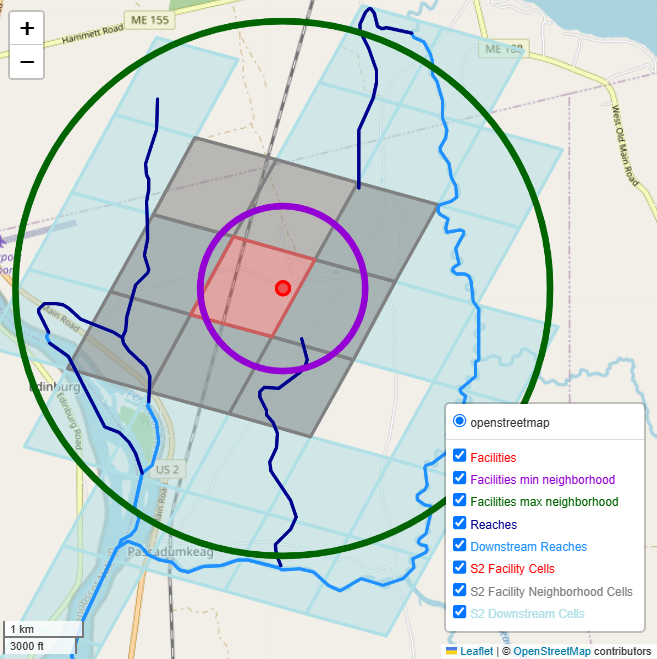
By including the eight S2 neighbors, we guarantee to find all stream reaches within a radius equal to the length of the shortest side of the S2 cell, as illustrated in Figure 4 using the shortest side of the center (red) S2 cell as radius. A circle of this radius, centered at any point in the center S2 cell, will always be entirely within the S2 neighborhood. The green circle has a radius equal to twice the longer diagonal of the center S2 cell to guarantee that the entire eight-cell S2 neighborhood in fully included no matter where the circle is centered within the center S2 cell. Stream reaches outside it will never be deemed “near” the facility by the S2-based approach. Thus, the radii of the red and green circles describe the lower and upper bound of the proximity operation’s spatial precision.
Because our approach is agnostic of where a feature is within an S2 cell, it cannot search within a fixed radius around a point location but approximates the search area using grid cells. It limits spatial precision but gains efficiency because it avoids the need to compute distances or buffers on-the-fly. At query time, the set of S2 cells describing the proximal area can be retrieved from the Spatial KG and passed on to the Hydrology KG for retrieving the stream reaches that intersect those S2 cells (Query Segment 1, B1c, line 21).
5.3 Network Tracing and Network Distance: Trace stream reaches


The identified stream reaches from Query Segment 1 (denoted by variable ?s2_ds_reach and shown as dark blue lines in Figure 5(a)) serve as starting points for our network tracing task. The stream reaches are the smallest hydrological flow segments connected to one another via the relation hyf:downstreamFlowPath and its inverse hyf:upstreamFlowPath in SAWGraph, which are based on NHD’s downstream and upstream relations to define a flow direction. They allow the construction of longer flow paths, which are directed paths that each consist of a sequence of one or more stream reaches and can be traced upstream (i.e., from a sink to a source) or downstream (i.e., from a source to a sink). For our question, Block B1c of Query Segment 1 uses the Hydrology graph to trace the stream reaches downstream (light blue lines in Figure 5(a)) by exploiting the transitive closure of the hyf:downstreamFlowPath relation using SPARQL’s transitive path operator “+” (line 23). The same effect would be achieved by defining hyf:downstreamFlowPathTC as a transitive superproperty thereof in the ontology (see [20]), which is propagated and prematerialized during graph construction and, thus, even faster. Either approach provides a structured way to navigate the hydrological network and simulate flow paths originating from a given starting point.
It may not always be desirable to consider all stream reaches downstream of a given feature. Because the KG stores the length of each reach, it is possible to limit downstream reach to those within a chosen maximum flow path length. This can be accomplished by adding the subquery shown in Query Segment 2 to Block B1c of Query Segment 1 along with a filter to set the maximum length. The subquery takes a reach (?reach) that is near a facility along with any of its downstream reaches (?ds_reach), and then sums the lengths of all intermediate stream reaches (?f1). Because each stream reach is defined as downstream of itself (for this specific purpose), the total distance includes the entire lengths of both ends of the flow path. In the example, only flow paths shorter than 20 km are returned.
These kinds of tracing analyses can be expanded, for example, by using the S2 cells retrieved in Query Segment 1 to also identify potential hydrological connectivity – or at least proximity – between contaminated surface water bodies and groundwater aquifers. This could further improve contaminant tracing by locating groundwater resources that may be infiltrated by PFAS from nearby contaminated stream reaches.
5.4 Proximity and Spatial Intersection: Find relevant PFAS results
The final step in answering Question 1 focuses on retrieving PFAS-related data, such as water quality measurements or fish tissue contamination levels, from samples collected along the downstream reaches of the hydrological network. Since sampling observations and hydrological datasets are in distinct thematic layers, we can only establish meaningful correlations by first spatially linking them via the S2 cells as spatial reference entities. However, stream reaches are often represented as 1-dimensional geometric approximations of a water body’s central flow path, which exclude the width and area of the river. Consequently, sampling points, represented as 0-dimensional geometries, that were originally within the river’s boundaries may no longer intersect with the simplified line geometries. One approach to mitigate this issue is to apply a buffer around the stream reaches, approximating the river’s extent and improving the accuracy of the intersection. However, it may still miss sampling points located just outside along the shore. Another approach is to calculate the distance from each sampling point to the nearest stream reach and retrieve points within a reasonable threshold. However, both methods involve computationally expensive geometric operations, which can be impractical whenever the datasets become larger.
To overcome these limitations, our solution (see Query Segment 3) again leverages the S2 cells (variable ?s2_ds_reach from Query Segment 1) that intersect the downstream reach segments. These S2 cells act as approximate spatial buffers, enabling efficient filtering of PFAS sampling data without the need for computationally intensive geometric calculations. The query retrieves all sampling observations whose sampling points are within those S2 cells (lines 3–4). Lines 6 and 7 then retrieve information about their material sample type (e.g., water or fish) and Block B3b accesses the contamination observation results using the SOSA observation-measurement-result pattern [59].
5.5 Vector Overlay: Find impacted areas without public water supply
In addition to supporting spatial filtering and proximity tasks, the SRE+Topology approach also supports simplified and efficient proxies for more expensive spatial overlay operations such as polygon intersection, union and difference. We demonstrate this functionality by determining which of the reaches downstream from potentially polluting facilities are inside (intersection) or outside (difference operation) of community water supply service areas to address Question 2 introduced at the beginning of Section 5. It helps prioritize PFAS testing in areas without public drinking water access where residents typically rely on private wells that may be affected by the contaminated water table. Analogous to Query Segment 3, we take the S2 cell neighborhoods of all downstream reaches (?s2_ds_reach) as an approximate buffer, and overlay them with the (precomputed) S2 cells that overlap with any community water supply service area to determine the difference between the two sets of S2 cells to avoid computationally expensive spatial calculations.
This analysis is just one of many; Query Segment 3 could be expanded further by adding other environmental variables, such as soil type, precipitation, and land use, via federated querying of external graphs to put the contamination results (encoded by the variable ?measure) in context. It could guide testing and monitoring strategies by examining the correlations highly contaminated stream reaches exhibit with respect to, e.g., agricultural activity, population density, or industrial land use; or prioritize interventions by ranking regions by vulnerability based on observed contamination, environmental factors, and human exposure risks.
5.6 Comparison to GeoSPARQL Operations
For comparison we also implemented and executed Question 1 using on-the-fly GeoSPARQL functions and predicates to perform the same analysis though obtaining the precise rather than spatially approximated results222The original and optimized queries and their GeoSPARQL equivalents are available from https://github.com/SAWGraph/public/tree/main/UseCases/UC3-Tracing/UC3-CQ15/GIScience2025-queries.. The geometries of our features are stored in 3-D coordinates (latitude longitude WGS84), and therefore we use a proximity distance of 0.014 arc degrees, which is equivalent to approximately 1119.06 m in our study area at 44 degrees North latitude. To perform the equivalents of Query Segments 1 and 3 in GeoSPARQL we use a distance search (geof:distance) on facilities within Maine (geo:sfWithin) to find nearby stream reaches, follow them downstream, and then buffer downstream reaches to find sampling points within the downstream reach buffer. This query completes in 165s, compared to our equivalent S2-based query in Section 5.4, which completes in 21s when executed on the same server under the same conditions. The question as defined is limited to only converted paper manufacturing facilities in Maine, which encompasses only 10 facilities. When we expand this search to all facilities in Maine in industries suspected of using PFAS, which encompasses a total of 354 facilities, the GeoSPARQL query completes in approximately 84 minutes (1h 23m 55s) while the equivalent S2-based query takes less than 11 minutes (10m 39s). Both S2-based queries achieve an eightfold – almost an order of magnitude – speedup. More importantly, these improvements do not rely on using any internal quadtree or other specialized indexing data structure for encoding the S2 geometry. Thus, we would expect comparable performance of the SRE+Topology approach in other RDF graph databases regardless of whether they provide any kind of geospatial indexing or GeoSPARQL support. A much more comprehensive comparison will be part of future work.
6 Summary and Discussion
We have demonstrated how the SRE+Topology approach supports efficient execution of advanced geospatial questions, such as about environmental contamination, directly in a GeoKG without the need for specialized reasoners, spatial indexing, or the GeoSPARQL geometric operations. Our example questions about environmental contamination combine network analysis with intersection, proximity, and overlay operations. For example, knowledge about the hydrological network for contaminant transport is leveraged together with proximity information and spatial intersections to identify downstream contamination risks.
Executing such advanced geospatial analysis questions in a GeoKG using GeoSPARQL operations instead of the precomputed topological relations would require spatial indexing and/or expensive spatial computations for geometric overlays, buffering, and topological analysis across features from multiple geospatial data layers. In the SRE+Topology approach, these spatial tasks are addressed in a unified way that relies entirely on precomputed topological links between different features and S2 cells, eliminating the need for resource-intensive geometric operations at query time. Querying a large GeoKG via these links maintains computational efficiency while enabling complex analyses across large datasets and extensive geographic ranges. The SRE+Topology approach facilitates the construction of these queries within and across graphs using standard SPARQL constructs only, that is, without the need for GeoSPARQL, thereby democratizing geospatial analysis via GeoKGs. Morever, the proposed approach integrates the semantic representation afforded by GeoKGs with the analytic capabilities afforded by conventional GIS.
Furthermore, the SRE+Topology approach allows sharing spatial reference entities (SREs), such as S2 cells and administrative regions, across separate graphs. It offers a robust mechanism to distribute data into separate thematic GeoKGs while ensuring their spatial compatibility. Thereby, some of the scalability challenges related to graph construction, maintenance, storage, and querying experienced in KnowWhereGraph – which was constructed as a single monolithic GeoKG – can be overcome. With SRE+Topology, different thematic information, such as hydrological, environmental, or socio-economic information, can be stored in separate GeoKGs, each maintained by their respective data producers or owners. Through the precomputed topological relations between features from these independent graphs and the shared SREs, the GeoKGs can be queried jointly using SPARQL’s federation construct (SERVICE). This modular and distributed architecture supports the growth of these graphs and helps accommodate more diverse and dynamic spatial datasets.
The SRE+Topology approach is, by design, a compromise between a full explicit representation of topological relationships, which would be impractical, and the classical approach of computing spatial queries on-the-fly. This design naturally comes with some drawbacks, which we can only outline here but that require future study. The first is the computational and storage overhead caused by precomputing and storing the intersections of all features in the thematic GeoKGs with the spatial reference entities. The number of additional triples for representing the SREs is constant, thus it is critical to carefully select suitable reference entities. In SAWGraph, we choose level 13 S2 cells and level 3 administrative regions to strike a balance between spatial granularity and computational demands (storage and query processing times). The number of triples for representing the topological relations only grows linearly in terms of the number of geographic features stored across all thematic layers and can be distributed as well. Efficient precomputation may also be more problematic for highly dynamic datasets, as any updates require recomputing the stored topological relations, adding potentially significant maintenance overhead.
A related limitation concerns the afforded spatial granularity and thus spatial precision, in particular for queries that require precise geometric measures, such as distances or buffers. The supported spatial granularity is directly tied to the choice of S2 cell or administrative region level used as SREs. Rather than switching everything to finer-grained S2 cells (or other SREs), which would rapidly increase storage needs, a more flexible approach could leverage the hierarchical relations (e.g., kwg-ont:sfContains) between different levels of SREs to allow topologically linking thematic features to the level that best reflects the granularity of a specific thematic dataset. Another option is a hybrid approach, where the SRE+Topology approach is used to narrow the set of potential features of interest to a small subset of all features (e.g., all PFAS sample locations within the S2 neighbors that overlap a stream reach) before applying precise geometric operations, such as a distance function, to calculate the exact distance of each such sample location from the stream reach to determine whether to include or exclude the location. However, suitable querying approaches require careful design and testing to verify that they actually are more storage and/or time efficient. Finally, some spatial operations, such as those that construct new polygons from the intersection of existing polygons rather than just determining whether they intersect, cannot be easily implemented using only the SRE+Topology approach but would require a hybrid approach.
References
- [1] Agency for Toxic Substances and Disease Registry (ATSDR). Per- and polyflouroalkyl substances (PFAS) and your health, November 2024. URL: https://www.atsdr.cdc.gov/pfas/about/health-effects.html.
- [2] Chaitan Baru, Martin Halbert, Lara Campbell, Tess DeBlanc-Knowles, Jemin George, Wo Chang, Adam Pah, Douglas Maughan, Ilya Zaslavsky, Amanda Stathopoulos, et al. Open knowledge network roadmap: Powering the next data revolution. Technical report, National Science Foundation, 2022.
- [3] Robert Battle and Dave Kolas. GeoSPARQL: Enabling a geospatial semantic web. Semantic Web Journal, 3(4):355–370, 2011.
- [4] Dan Brickley and Ramanathan Guha. RDF vocabulary description language 1.0: RDF schema. W3C recommendation, W3C, February 2004. URL: https://www.w3.org/TR/2004/REC-rdf-schema-20040210/.
- [5] B. Brodaric, E. Boisvert, Chery. L., P. Dahlhaus, S. Grellet, A. Kmoch, F. Letourneau, J. Lucido, B. Simons, and B. Wagner. Enabling global exchange of groundwater data: GroundWaterML2 (GWML2). Hydrogeology Journal, 26(3):733–741, 2018. doi:10.1007/s10040-018-1747-9.
- [6] Boyan Brodaric and Torsten Hahmann. Towards a foundational hydro ontology for water data interoperability. In 11th Internationa Conference on Hydroinformatics (HIC-2014), pages 2911–2915, 2014.
- [7] Boyan Brodaric, Torsten Hahmann, and Michael Gruninger. Water features and their parts. Applied Ontology, 14(1):1–42, 2019. doi:10.3233/AO-190205.
- [8] Ying Chen. Enhancing Spatial Query Efficiency Through Dead Space Indexing in Minimum Bounding Boxes. PhD thesis, University of Waterloo, 2024.
- [9] James Cheng, Yiping Ke, and Wilfred Ng. Efficient query processing on graph databases. ACM Transactions on Database Systems (TODS), 34(1):1–48, 2009. doi:10.1145/1508857.1508859.
- [10] Eliseo Clementini, Paolino Di Felice, and Peter van Oosterom. A small set of formal topological relationships suitable for end-user interaction. In David Abel and Beng Chin Ooi, editors, Advances in Spatial Databases, pages 277–295. Springer, 1993. doi:10.1007/3-540-56869-7_16.
- [11] Data Commons. Data commons 2025. URL: https://datacommons.org.
- [12] Irina Dornblut and Robert Atkinson. HY_Features: a geographic information model for the hydrology domain. Technical Report GRDC 43r1, Global Runoff Data Centre, November 2013.
- [13] Martin Doyle and Kyle Onda. Internet of water: Research and development toward a linked data system and foundational knowledge network for the internet of water. Technical report, NC WRRI, 2023.
- [14] Sebastián Ferrada, Benjamin Bustos, and Aidan Hogan. Similarity joins and clustering for SPARQL. Semantic Web, 15(5):1701–1732, 2024. doi:10.3233/SW-243540.
- [15] GADM maps and data. URL: https://gadm.org/index.html.
- [16] George Garbis, Kostis Kyzirakos, and Manolis Koubarakis. Geographica: A benchmark for geospatial RDF stores. In 12th International Semantic Web Conference (ISWC 2013), pages 343–359. Springer, 2013.
- [17] Torsten Hahmann. Ontology. In B.S. Daya Sagar, Qiuming Cheng, Jennifer McKinley, and Frits Agterberg, editors, Encyclopedia of Mathematical Geosciences, pages 1–5. Springer, 2021. doi:10.1007/978-3-030-26050-7_231-1.
- [18] Torsten Hahmann and Boyan Brodaric. The void in hydro ontology. In 12th International Conference on Formal Ontology in Information Systems (FOIS-12), pages 45–58. IOS Press, 2012. doi:10.3233/978-1-61499-084-0-45.
- [19] Torsten Hahmann, Pascal Hitzler, Hande Küçük McGinty, Ganga Hettiarachchi, Onur Apul, et al. Safe Agricultural Products and Water Graph (SAWGraph): An Open Knowledge Network to Monitor and Trace PFAS and Other Contaminants in the Nation’s Food and Water Systems. URL: https://sawgraph.github.io/.
- [20] Torsten Hahmann and David K Kedrowski. An ontology and geospatial knowledge graph for reasoning about cascading failures. In 16th International Conference on Spatial Information Theory (COSIT 2024), pages 21:1–9. Schloss Dagstuhl – Leibniz-Zentrum für Informatik, 2024. doi:10.4230/LIPIcs.COSIT.2024.21.
- [21] Torsten Hahmann, Katrina Schweikert, Shirly Stephen, and David Kedrowski. ContaminOSO: Ontological foundations and key design choices for an ontology for environmental contaminant data. In 25th International Conference on Formal Ontology in Inf. Systems (FOIS-25). IOS Press, 2025 (to appear).
- [22] Torsten Hahmann and Shirly Stephen. Using a hydro-reference ontology to provide improved computer-interpretable semantics for the groundwater markup language (GWML2). International Journal of Geographic Information Science, 32(6):1138–1171, 2018. doi:10.1080/13658816.2018.1443751.
- [23] Pascal Hitzler, Bijan Parsia, Peter Patel-Schneider, and Sebastian Rudolph. OWL 2 Web Ontology Language Primer (Second Edition). https://www.w3.org/TR/owl2-primer/, 2012. https://www.w3.org/TR/owl2-primer/.
- [24] Ralph Hodgson, Paul J. Keller, Jack Hodges, and Jack Spivak. QUDT: Quantities, units, dimensions and types, 2012. URL: https://qudt.org/.
- [25] Weiming Huang, Syed Amir Raza, Oleg Mirzov, and Lars Harrie. Assessment and benchmarking of spatially enabled RDF stores for the next generation of spatial data infrastructure. ISPRS International Journal of Geo-Information, 8(7):310, 2019. doi:10.3390/IJGI8070310.
- [26] Theofilos Ioannidis. Geospatial RDF stores. In Geospatial Data Science: A Hands-on Approach for Building Geospatial Applications Using Linked Data Technologies, pages 221–240. Association for Computing Machinery, 2023.
- [27] Theofilos Ioannidis, George Garbis, Kostis Kyzirakos, Konstantina Bereta, and Manolis Koubarakis. Evaluating geospatial RDF stores using the benchmark Geographica 2. Journal on Data Semantics, 10(3):189–228, 2021. doi:10.1007/S13740-021-00118-X.
- [28] Krzysztof Janowicz, Armin Haller, Simon J.D. Cox, Danh Le Phuoc, and Maxime Lefrançois. Sosa: A lightweight ontology for sensors, observations, samples, and actuators. Journal of Web Semantics, 56:1–10, 2019. doi:10.1016/j.websem.2018.06.003.
- [29] Krzysztof Janowicz, Pascal Hitzler, Wenwen Li, Dean Rehberger, Mark Schildhauer, Rui Zhu, Cogan Shimizu, Colby Fisher, Ling Cai, Gengchen Mai, et al. Know, Know Where, KnowWhereGraph: A densely connected, cross-domain knowledge graph and geo-enrichment service stack for applications in environmental intelligence. AI Magazine, 43(1):30–39, 2022. doi:10.1609/AIMAG.V43I1.19120.
- [30] Peiquan Jin, Xike Xie, Na Wang, and Lihua Yue. Optimizing R-tree for flash memory. Expert Systems with Applications, 42(10):4676–4686, 2015. doi:10.1016/J.ESWA.2015.01.011.
- [31] J Michael Johnson, Tom Narock, Justin Singh-Mohudpur, Doug Fils, Keith Clarke, Siddharth Saksena, Adam Shepherd, Sankar Arumugam, and Lilit Yeghiazarian. Knowledge graphs to support real-time flood impact evaluation. AI Magazine, 43(1):40–45, 2022. URL: https://ojs.aaai.org/index.php/aimagazine/article/view/19121.
- [32] Milos Jovanovik, Timo Homburg, and Mirko Spasić. A GeoSPARQL compliance benchmark. ISPRS International Journal of Geo-Information, 10(7):487, 2021. doi:10.3390/IJGI10070487.
- [33] Sudarshan Kurwadkar, Jason Dane, Sushil R Kanel, Mallikarjuna N Nadagouda, Ryan W Cawdrey, Balram Ambade, Garrett C Struckhoff, and Richard Wilkin. Per-and polyfluoroalkyl substances in water and wastewater: A critical review of their global occurrence and distribution. Science of The Total Environment, 809:151003, 2022.
- [34] Wenwen Li, Sizhe Wang, Sheng Wu, Zhining Gu, and Yuanyuan Tian. Performance benchmark on semantic web repositories for spatially explicit knowledge graph applications. Computers, Environment and Urban Systems, 98:101884, 2022. doi:10.1016/J.COMPENVURBSYS.2022.101884.
- [35] Jiajun Liu, Haoran Li, Yong Gao, Hao Yu, and Dan Jiang. A geohash-based index for spatial data management in distributed memory. In 22nd International Conference on Geoinformatics, pages 1–4, 2014. doi:10.1109/GEOINFORMATICS.2014.6950819.
- [36] Junnan Liu, Haiyan Liu, Xiaohui Chen, Xuan Guo, Qingbo Zhao, Jia Li, Lei Kang, and Jianxiang Liu. A heterogeneous geospatial data retrieval method using knowledge graph. Sustainability, 13(4):2005, 2021.
- [37] Gengchen Mai, Yingjie Hu, Song Gao, Ling Cai, Bruno Martins, Johannes Scholz, Jing Gao, and Krzysztof Janowicz. Symbolic and subsymbolic GeoAI: Geospatial knowledge graphs and spatially explicit machine learning. Transactions in GIS, 26(8):3118–3124, 2022. doi:10.1111/TGIS.13012.
- [38] Gengchen Mai, Krzysztof Janowicz, Bo Yan, and Simon Scheider. Deeply integrating linked data with geographic information systems. Transactions in GIS, 23(3):579–600, 2019. doi:10.1111/TGIS.12538.
- [39] Gengchen Mai, Krzysztof Janowicz, Rui Zhu, Ling Cai, and Ni Lao. Geographic question answering: challenges, uniqueness, classification, and future directions. In 24th AGILE Conference on Geographic Information Science, pages 8:1–21. Copernicus Publications, 2021. doi:10.5194/agile-giss-2-8-2021.
- [40] Maine Geological Survey (MGS). Water well database. https://www.maine.gov/dacf/mgs/pubs/digital/well.htm. Accessed 3 October 2023.
- [41] National Science Foundation. The Proto-OKN initiative, 2023. URL: https://www.proto-okn.net/.
- [42] Maine Department of Environmental Protection. Enivornmental and geographic analysis database EGAD. https://www.maine.gov/dep/maps-data/egad/. March 2024 release.
- [43] Open Geospatial Consortium. OGC GeoSPARQL - A Geographic Query Language for RDF Data. Open Geospatial Consortium, URL http://www.opengeospatial.org/standards/requests/80, 2011. Document 11-052r3.
- [44] Open Street Map Foundation. OpenStreetMap. URL: https://www.openstreetmap.org/.
- [45] Hoan Nguyen Mau Quoc and Danh Le Phuoc. An elastic and scalable spatiotemporal query processing for linked sensor data. In 11th International Conference on Semantic Systems (Semantics’15), pages 17–24, 2015. doi:10.1145/2814864.281486.
- [46] Amir Raza. Comparison of geospatial support in rdf stores: Evaluation for icos carbon portal metadata. Master Thesis in Geographical Information Science, 2019.
- [47] RDF Core Working Group. Resource Description Framework (RDF): Concepts and Abstract Syntax. http://www.w3.org/TR/2004/REC-rdf-concepts-20040210/, February 2004.
- [48] Blake Regalia, Krzysztof Janowicz, and Grant McKenzie. Computing and querying strict, approximate, and metrically refined topological relations in linked geographic data. Transactions in GIS, 23(3):601–619, 2019. doi:10.1111/TGIS.12548.
- [49] Philippe Rigaux, Michel Scholl, and Agnes Voisard. Spatial databases: with application to GIS. Elsevier, 2002.
- [50] S2 Geometry. URL: http://s2geometry.io/.
- [51] Marina Schauffler. Testing the waters: Tracing the movement of PFAS into waterways and wildlife, 2023. URL: https://themainemonitor.org/testing-the-waters-tracing-the-movement-of-pfas-into-waterways-and-wildlife/.
- [52] Katrina Schweikert, David Kedrowski, Shirly Stephen, and Torsten Hahmann. SAWGraph Example Geospatial SPARQL Queries. Software, version 1.1, swhId: swh:1:dir:678ee78feb48f235c42bd5722e4c19f81f91f9dc (visited on 2025-07-30). URL: https://github.com/SAWGraph/public/tree/main/UseCases/UC3-Tracing/UC3-CQ15/GIScience2025-queries, doi:10.4230/artifacts.24220.
- [53] Chandan Sharma, Pierre Genevès, Nils Gesbert, and Nabil Layaïda. Schema-based query optimisation for graph databases. arXiv preprint arXiv:2403.01863, 2024. doi:10.48550/arXiv.2403.01863.
- [54] Cogan Shimizu, Shirly Stephen, Adrita Barua, Ling Cai, Antrea Christou, Kitty Currier, Abhilekha Dalal, Colby K Fisher, Pascal Hitzler, Krzysztof Janowicz, et al. The KnowWhereGraph ontology. Journal of Web Semantics, page 100842, 2024.
- [55] Amila O. De Silva, James M. Armitage, Thomas A. Bruton, Clifton Dassuncao, Wendy Heiger-Bernays, Xindi C. Hu, Anna Kärrman, Barry Kelly, Carla Ng, Anna Robuck, Mei Sun, Thomas F. Webster, and Elsie M. Sunderland. PFAS exposure pathways for humans and wildlife: A synthesis of current knowledge and key gaps in understanding. Environmental Toxicology and Chemistry, 40:631–657, March 2021. doi:10.1002/etc.4935.
- [56] Shirly Stephen, Mitchell Faulk, Krzysztof Janowicz, Colby Fisher, Thomas Thelen, Rui Zhu, Pascal Hitzler, Cogan Shimizu, Kitty Currier, Mark Schildhauer, et al. The S2 hierarchical discrete global grid as a nexus for data representation, integration, and querying across geospatial knowledge graphs. arXiv preprint, 2024. arXiv:2410.14808.
- [57] Shirly Stephen, Torsten Hahmann, and David K. Kedrowski. The SAWGraph spatial ontology. URL: https://raw.githubusercontent.com/SAWGraph/geospatial-kg/refs/heads/main/ontologies/sawgraph-spatial-ontology.ttl.
- [58] Markus Stocker, Andy Seaborne, Abraham Bernstein, Christoph Kiefer, and Dave Reynolds. SPARQL basic graph pattern optimization using selectivity estimation. In 17th International Conference on World Wide Web (WWW 2008), pages 595–604. ACM, 2008. doi:10.1145/1367497.136757.
- [59] Kerry Taylor, Simon Cox, Krzysztof Janowicz, Maxime Lefrançois, Danh Le Phuoc, and Armin Haller. Semantic sensor network ontology. W3C recommendation, W3C, October 2017. URL: https://www.w3.org/TR/2017/REC-vocab-ssn-20171019/.
- [60] Kingsley Wiafe-Kwakye, Torsten Hahmann, and Kate Beard. An ontology design pattern for spatial and temporal aggregate data (STAD). In 13th Workshop on Ontology Design and Patterns (WOP 2022) at the 21st International Semantic Web Conference (ISWC 2022). CEUR-WS.org, 2022. URL: https://ceur-ws.org/Vol-3352/pattern4.pdf.
- [61] Marc Wick. GeoNames. URL: https://www.geonames.org/.
- [62] Mark D Wilkinson, Michel Dumontier, IJsbrand Jan Aalbersberg, Gabrielle Appleton, Myles Axton, Arie Baak, Niklas Blomberg, Jan-Willem Boiten, Luiz Bonino da Silva Santos, Philip E Bourne, et al. The FAIR guiding principles for scientific data management and stewardship. Scientific data, 3(1):1–9, 2016.
- [63] Rui Zhu. Geospatial knowledge graphs. arXiv preprint arXiv:2405.07664, 2024. doi:10.48550/arXiv.2405.07664.
Appendix A Namespaces for ontologies and SPARQL queries
| PREFIX | Ontology namespace (URL) |
|---|---|
| coso: | http://w3id.org/coso/v1/contaminoso# |
| fio: | http://w3id.org/fio/v1/fio# |
| geo: | http://www.opengis.net/ont/geosparql# |
| hyf: | https://www.opengis.net/def/schema/hy_features/hyf/ |
| kwg-ont: | http://stko-kwg.geog.ucsb.edu/lod/ontology/ |
| kwgr: | http://stko-kwg.geog.ucsb.edu/lod/resource/ |
| me_egad: | http://w3id.org/sawgraph/v1/me-egad# |
| naics: | http://w3id.org/fio/v1/naics# |
| nhdplusv2: | http://w3id.org/hyfo/v1/nhdplusv2# |
| qudt: | http://qudt.org/schema/qudt/ |
| spatial: | http://purl.org/spatialai/spatial/spatial-full# |
Appendix B Visualization of the Contaminant Tracing Results for the State of Maine
