Reachability in Deletion-Only Chemical Reaction Networks

Let $\mathrm{\Lambda }=\{{\lambda }_1,{\lambda }_2,\mathrm{\dots },{\lambda }_{|\mathrm{\Lambda }|}\}$ denote some ordered alphabet of species. A configuration $\overrightarrow{C}\in {\mathbb{N}}^{\mathrm{\Lambda }}$ is a length-$|\mathrm{\Lambda }|$ vector of non-negative integers where $\overrightarrow{C}[i]$ denotes the number of copies of species ${\lambda }_i$. For a species ${\lambda }_i\in \mathrm{\Lambda }$, we denote the configuration consisting of a single copy of ${\lambda }_i$ and no other species as ${\overrightarrow{\lambda }}_i$. A rule or reaction is represented as an ordered pair $\gamma =(\overrightarrow{R},\overrightarrow{P})\in {\mathbb{N}}^{\mathrm{\Lambda }}\times {\mathbb{N}}^{\mathrm{\Lambda }}$. $\overrightarrow{R}$ contains the minimum counts of each reactant species necessary for reaction $\gamma$ to occur, where reactant species are either consumed by the rule in some count or leveraged as catalysts (not consumed); in some cases a combination of the two. The product vector $\overrightarrow{P}$ has the count of each species produced by the application of rule $\gamma$, effectively replacing vector $\overrightarrow{R}$. The species corresponding to the non-zero elements of $\overrightarrow{R}$ and $\overrightarrow{P}$ are termed reactants and products of $\gamma$, respectively.

The application vector of $\gamma$ is $\overrightarrow{P}-\overrightarrow{R}$, which shows the net change in species counts after applying rule $\gamma$ once. For a configuration $\overrightarrow{C}$ and rule $\gamma$, we say $\gamma$ is applicable to $\overrightarrow{C}$ if $\overrightarrow{C}[i]\ge \overrightarrow{R}[i]$ for all $i\in \mathrm{\Lambda }$, and we define the application of $\gamma$ to $\overrightarrow{C}$ as the configuration ${\overrightarrow{C}}^{\prime }=\overrightarrow{C}+\overrightarrow{P}-\overrightarrow{R}$. For a set of rules $\mathrm{\Gamma }$, a configuration $\overrightarrow{C}$, and rule $\gamma \in \mathrm{\Gamma }$ applicable to $\overrightarrow{C}$ that produces ${\overrightarrow{C}}^{\prime }=\overrightarrow{C}+\overrightarrow{P}-\overrightarrow{R}$, we say $\overrightarrow{C}{\to }_{\mathrm{\Gamma }}^1{\overrightarrow{C}}^{\prime }$, a relation denoting that $\overrightarrow{C}$ can transition to ${\overrightarrow{C}}^{\prime }$ by way of a single rule application from $\mathrm{\Gamma }$. We further use the notation $\overrightarrow{C}{\to }_{\mathrm{\Gamma }}^{\ast }{\overrightarrow{C}}^{\prime }$ to signify the transitive closure of ${\to }_{\mathrm{\Gamma }}^1$ and say ${\overrightarrow{C}}^{\prime }$ is reachable from $\overrightarrow{C}$ under $\mathrm{\Gamma }$, i.e., ${\overrightarrow{C}}^{\prime }$ can be reached by applying a sequence of applicable rules from $\mathrm{\Gamma }$ to initial configuration $\overrightarrow{C}$. Here, we use the following notation to depict a rule $(\overrightarrow{R},\overrightarrow{P})$: $\overrightarrow{R}[1]{\lambda }_1+\mathrm{\cdots }+\overrightarrow{R}[|\mathrm{\Lambda }|]{\lambda }_{|\mathrm{\Lambda }|}\to \overrightarrow{P}[1]{\lambda }_1+\mathrm{\cdots }+\overrightarrow{P}[|\mathrm{\Lambda }|]{\lambda }_{|\mathrm{\Lambda }|}$. For example, a rule turning two copies of species $H$ and one copy of species $O$ into one copy of species $W$ would be written as $2H+O\to W$.

A configuration is called terminal with respect to a CRN $(\mathrm{\Lambda },\mathrm{\Gamma })$ if no rule $\gamma$ can be applied to it. An initial configuration $\overrightarrow{A}$ and CRN $(\mathrm{\Lambda },\mathrm{\Gamma })$ is said to be bounded if a terminal configuration is guaranteed to be reached within some finite number of rule applications starting from $\overrightarrow{A}$. We denote the set of reachable configurations of a CRN as $REAC{H}_{\overrightarrow{A},\mathrm{\Lambda },\mathrm{\Gamma }}$. We define the subset of reachable configurations that are terminal as $TER{M}_{\overrightarrow{A},\mathrm{\Lambda },\mathrm{\Gamma }}$.

For each vertex $v\in V$, we create the species $v$, $v_R$, $v_G$, and $v_B$. $v_C$ represents an assignment of color $C\in \{R,G,B\}$ to vertex $v$; the $v$ species will be used to represent assigning only one color to vertex $v$ through specific reactions. We also create the species $X$ to verify that a corresponding color assignment of $G$ in ${𝒞}_{𝒮}$ has no adjacent vertices that share a color.

In step one (or ${\overrightarrow{S}}_0$), for each $v\in V$, we add two copies of $v$ and one copy of $v_R$, $v_G$, and $v_B$. We also create the assignment rule $v+v_C\to \mathrm{\varnothing }$ for each $C\in \{R,G,B\}$. Two of the three assignment rules created for $v$ are applied to its respective species copies, consuming all $v$ copies and two of the three copies of $v_C$. The remaining $v_C$ copy then corresponds to assigning vertex $v$ the color $C$. Additionally, for each edge $(i,j)\in E$ and $C\in \{R,G,B\}$, we create the edge rule $i_C+j_C\to \mathrm{\varnothing }$. If the remaining copy of both $i_C$ and $j_C$ share a color $C$, they will be deleted by one of the edge rules.

In the second step (${\overrightarrow{S}}_1$), we introduce $|V|$ copies of the species $X$. We also construct the verification rule $v_C+X\to \mathrm{\varnothing }$ for each $v\in V$ and $C\in \{R,G,B\}$. All existing copies of $v_C$ will be consumed by a $X$ species. Thus, any remaining copies of $X$ in the terminal configuration indicates that some $v_C$ copies were deleted by an edge rule.

We reduce from the graph 3-colorability problem. Given an instance of 3-COL $⟨G⟩$, we convert $G$ into a $2$-step $(2,0)$ CRN ${𝒞}_{𝒮}$, following the construction outlined above, and set $\overrightarrow{A}={\overrightarrow{S}}_0$ and $\overrightarrow{B}$ to the empty configuration $\overrightarrow{0}$.

Assume there exists a color assignment in $G$ where no adjacent vertices share a color. By the construction of ${𝒞}_{𝒮}$, a sequence of assignment rules can be applied in $\overrightarrow{A}$ that results in a configuration of one copy of $v_C$ for each vertex that matches the color assignment in $G$. Denote this new configuration ${\overrightarrow{S}}_0^{\prime }$. Since no adjacent vertices share a color in $G$, no edge rule will be applied in ${\overrightarrow{S}}_0^{\prime }$, keeping the count of the $v_C$ copies to $|V|$. ${𝒞}_{𝒮}$ then transitions to $\overrightarrow{S_1}$, introducing the $|V|$ $X$ copies. Since $|V|$ $V_C$ copies were preserved, all $v_C$ and $X$ copies are deleted by verification reactions to reach the final configuration $\overrightarrow{0}=\overrightarrow{B}$.

Assume there exists a sequence of applicable rules in ${𝒞}_{𝒮}$ that reaches $\overrightarrow{B}$ from $\overrightarrow{A}$. First, removing all $v$ species can only be accomplished by applying a sequence of assignment rules. The resulting configuration ${\overrightarrow{S}}_0^{\prime }$ is $|V|$ $v_C$ copies. Assume no edge rule can be applied in ${\overrightarrow{S}}_0^{\prime }$. By the construction of ${𝒞}_{𝒮}$, this implies that the matching color assignment in $G$ also does not have adjacent vertices sharing colors. We then add $|V|$ $X$ copies at the second step, resulting in the deletion of all $v_C$ and $X$ copies in the system by the verification rules, resulting in a final terminal configuration of $\overrightarrow{0}$. If an edge rule was applied in ${\overrightarrow{S}}_0^{\prime }$, at least two $v_C$ copies were removed, causing the final count of $X$ to be greater than $0$. Note that applying an edge rule before an assignment rule also guarantees $\overrightarrow{0}$ cannot be reached, as either 1) the assignment rules for the affected $v_C$ copies are then applied, removing those copies and consequentially preventing some $X$ copies from being deleted, or 2) more edge rules are applied on the affected $v_C$ copies, which prevents all $v$ copies from being deleted. Therefore, the only way for ${𝒞}_{𝒮}$ to reach $\overrightarrow{0}=\overrightarrow{B}$ is for a color assignment to exist on all vertices in $G$ where no adjacent vertices share a color.

Theorem 7 shows reachability with void step CRN systems to be in NP. $◀$

We will refer to a node which satisfies one of these conditions as a root node. A path from species ${\lambda }_i$ to a root node ${\lambda }_r$ means that we can delete enough copies of ${\lambda }_i$ to reach the target configuration. We will prove this recursively, inducing over the length of the path from ${\lambda }_i$ to ${\lambda }_r$, to create a reaction sequence through this process with our base case being the end of the sequence.

For our base case, any node ${\lambda }_i={\lambda }_r$ can reach the target amount if it satisfies a condition in the Lemma statement. In Case 1, the number of species in the starting configuration is already the target amount so the claim is trivially true. In Case 2, we may use copies of the species ${\lambda }_j$ to delete ${\lambda }_i$ using the leftover species in the target configuration. In Case 3, the species may delete itself to reach the target amount.

For our inductive case, assume that there exists a reachable configuration such that any species ${\lambda }_k$ with a shortest path of length $\le l$ to a node ${\lambda }_r$ can be reduced to the target amount $\overrightarrow{B}[k]$. For a species ${\lambda }_i$ with a shortest path of length $l+1$, there exists an edge to a species ${\lambda }_k$ with length $l$. We can use the reaction ${\lambda }_i+{\lambda }_k\to {\lambda }_k$ to decrease ${\lambda }_i$ to $\overrightarrow{B}[i]$ copies at the start of the current sequence. It remains to prove that removing these copies does not affect anything later in the sequence. If the closest node ${\lambda }_r$ falls under case 1 or 3 then removing ${\lambda }_i$ does not affect it. If the closest node is case 2 and ${\lambda }_i={\lambda }_j$, the species ${\lambda }_i$ is the one used to remove ${\lambda }_r$; thus, the condition $\overrightarrow{B}[j]\ge 1$ means that we leave at least a single copy in the configuration that can be used to delete ${\lambda }_r$.

If a node does not have a path to a root node, then it either does not have any outgoing edges, or all of its outgoing edges are part of some cycle where all nodes along each cycle have a target count of $0$. As a result, if the node does not fall into case 1, there is no way of reducing the respective species to its target count without leaving some other species unsatisfied. $◀$

We will show that we can decide whether a node has no path to a root in log space; thus reachability is in coNL $=$ NL. We non-deterministically check a species ${\lambda }_i$, then for every node ${\lambda }_j$ reachable from ${\lambda }_i$ in the implication graph, we check if ${\lambda }_j$ satisfies any of the conditions in Lemma 10. If we do not find such a node ${\lambda }_j$, then we reject.

If any node does not have a path to a root node, then some branch of this algorithm will reject. Checking each path can be done in NL as this is a directed graph. Checking if a node is a root node can be done in log space as it only involves edge queries and queries to the target configuration. $◀$

We now show that adding an extra step turns the problem NP-complete, as with $(2,0)$ CRN systems. Here, we reduce from the classic 3SAT problem. Given an instance of 3SAT $⟨\mathrm{\Phi }⟩$, we construct a $(2,1)$ $2$-step CRN ${𝒞}_{𝒮}$ as follows.

For each variable $x_i$, we create a pair of species $T_i$ and $F_i$, which represents assigning $x_i$ a value of true or false, respectively. Additionally, for each clause $c_j$, we create the species $C_j$. The presence of a copy of $C_j$ in a configuration of ${𝒞}_{𝒮}$ indicates $c_j$ has yet to be satisfied by one of its assigned variables. Finally, we create the species $X$ for “clean-up” procedures.

In the first step $({\overrightarrow{S}}_0)$, for each variable $x_i$, we introduce one copy of $T_i$ and $F_i$. We also create a pair of assignment rules, one to represent assigning true to $x_i$ ($T_i+F_i\to T_i$) and one for assigning false ($T_i+F_i\to F_i$). One of two assignment reactions will be applied to the copies of $T_i$ and $F_i$; the non-deleted copy represents assigning $x_i$ the corresponding boolean value.

In the second step $({\overrightarrow{S}}_1)$, we add a single copy of a clause species $C_j$ for each clause $c_j$ and a single copy of $X$. Additionally, given a clause $c_j$ and a variable of the clause $x_k\in (x_a,x_b,x_c)$, $3$ separate verification rules created of the form $C_j+T_k\to T_k$ (for non-negated variables) or $C_j+F_k\to F_k$ (for negated variables). If $T_k$/$F_k$ is still present in ${𝒞}_{𝒮}$, then $C_j$ will be consumed by that species. Finally, for each variable $x_i$, we create the cleaning rules $X+T_i\to X$ and $X+F_i\to X$ to consume all present copies of $T_i$ and $F_i$. Any $C_j$ species remaining in ${𝒞}_{𝒮}$ after the application of the cleaning rules indicates that it could not be deleted by a verification rule.

We reduce from 3SAT. Given an instance of 3SAT $⟨\mathrm{\Phi }⟩$, we convert $\mathrm{\Phi }$ into a $2$-step $(2,1)$ CRN ${𝒞}_{𝒮}$ via the reduction from above. Let $\overrightarrow{A}={\overrightarrow{S}}_0$ and $\overrightarrow{B}$ be a single copy of $X$ ($\overrightarrow{X}$).

Assume there exists an assignment of variables that satisfies $\mathrm{\Phi }$ to true. A sequence of assignment reactions can be then performed in ${\overrightarrow{S}}_0$ that results in a configuration with only one $T_i/F_i$ copy for each variable that matches the variable assignment. In the second step, by the construction of ${𝒞}_{𝒮}$, since the assignment satisfies $\mathrm{\Phi }$, each introduced copy of $C_j$ can be deleted with a verification reaction. Finally, the added $X$ copy deletes all remaining literal species. The final configuration of ${𝒞}_{𝒮}$ is then $\overrightarrow{X}$.

Assume there exists a sequence of applicable rules in ${𝒞}_{𝒮}$ that reaches $\overrightarrow{B}$ from $\overrightarrow{A}$. First, a sequence of assignment reactions can be performed in ${\overrightarrow{S}}_0$ that consumes one of the $T_i$ and $F_i$ copy for each variable. We then add one copy of each $C_j$ species and one copy of $X$ in the second step. Assume all $C_j$ copies can be consumed by a verification reaction. By the construction of ${𝒞}_{𝒮}$, this implies that there exists an assignment of variables in $\mathrm{\Phi }$ that evaluates the formula to true. The $X$ copy can delete the remaining $X_i/F_i$ copies with cleanup rules to reach the final configuration $\overrightarrow{X}$. If a $C_j$ copy could not be removed, this implies that the variable assignment couldn’t satisfy the corresponding clause. Therefore, the only way for ${𝒞}_{𝒮}$ to reach $\overrightarrow{X}=\overrightarrow{B}$ is for an assignment of variables in $\mathrm{\Phi }$ to exist that satisfies all clauses of the formula.

Theorem 7 shows reachability with void step CRN systems to be in NP. $◀$

For simplicity, let $n=|\mathrm{\Lambda }|$. Assume there exists a sequence of reactions $a_1{r}_1,\mathrm{\dots },$ $a_{n+1}{r}_{n+1}$ for a CRN $𝒞$ with set of species $\mathrm{\Lambda }$ and set of rules $\mathrm{\Gamma }$ that takes some initial configuration $\overrightarrow{A}$ to configuration $\overrightarrow{B}$, where $a_1,\mathrm{\dots },a_{n+1}$ are positive integers (denoting how many times to apply each rule) and $r_1,\mathrm{\dots },r_{n+1}$ are rules in $\mathrm{\Gamma }$. There must then exist some species $s$ that gets consumed by 2 rules $r_i$ and $r_j$, where . Let $s^i$, $s^x$ and $s^f$ denote the initial, intermediate and final counts of species $s$, where $r_i$ reduces $s$ from $s^i$ to $s^x$ and $r_j$ reduces $s$ from $s^x$ to $s^f$. Since $s^i>s^x$, any rule $r_l$, where $l>i$, that uses $s$ with count $s^x$ can also use $s$ with count $s^i$. Thus, rule $r_i$ is not needed. $◀$

Let $\mathrm{\Gamma }$ denote the set of rules. We can use a dynamic programming approach to solve the problem. Construct an $|\mathrm{\Lambda }|\times (|\mathrm{\Lambda }|+1)$ table $D(s,j)$ of boolean entries, where each row represents a different species. Reduce the count of each species to $max(k,s^f)$, where $s^f$ represents the final count of species $s$, if there exists a rule that can do so. Starting from the first column $j=0$, place a $1$ if the respective species is already in its final count. Then, for each entry $D(s,j)$, place a $1$ if $D(s,j-1)$ is a $1$ or if there exists a reaction $\gamma \in \mathrm{\Gamma }$ that reduces $s$ to its final count, where all the reactants of $\gamma$ have either reached their final counts or will not prevent the reaction from occurring once they do. If column $|\mathrm{\Lambda }|+1$ contains all 1’s, then reachability is possible. Otherwise, it is not.

By Lemma 19, a solution to the problem requires at most $|\mathrm{\Lambda }|$ unique reactions, where each reaction directly reduces each species from its initial counts to its final counts. Thus, finding a solution to the problem takes at most $|\mathrm{\Lambda }|$ steps since we are implicitly selecting at least one reaction per column. This results in $|\mathrm{\Lambda }|+1$ columns, with the first column representing the initial configuration.

Since every rule is a catalytic void rule, there must exist an ordering of reactions such that some reactions can occur first without impeding other species from getting reduced to their final counts. A bottom-up approach can be used to find this ordering, starting with the reactions that can be put off until later and working up to the reactions that must occur first. In table $D$, this ordering is implicitly represented between columns, with the reactions between the rightmost columns being the ones we do first. Any species with final count greater than $k$ is reduced before the algorithm is run if there exists an applicable rule, as reducing this species count does not prevent any other rule from occurring. Filling $D$ takes at most $O({|\mathrm{\Lambda }|}^2|\mathrm{\Gamma }|)$ steps. Hence, reachability is solvable in polynomial time. $◀$

This follows from Theorem 20. Since we are considering a rule set $\mathrm{\Gamma }$ where the size of each rule $\gamma \in \mathrm{\Gamma }$ is $\le k$, reducing each initial species count to $\max (k,s^f)$ guarantees that any $r$ that needs $s$ will be able to occur. The algorithm remains the same. $◀$

Follows from Theorem 12. $◀$

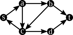
We create a species for every path through a vertex (unless it starts at $t$ or goes back to $s$). For example, looking at Figure 3, for vertex $b$, we create two species $S_{a,b,c}$ and $S_{a,b,t}$, where the notation denotes the vertex it came from, the vertex itself, and the vertex it goes to. With a maximum in/out degree of two, for each vertex, there are at most 4 paths through the vertex. In general, for each vertex $j\in V$, we create the species $S_{i,j,k}$ where $(i,j),(j,k)\in E$ and $k\ne s$, $i\ne t$. For $s,t$, we just have $S_s$ and $S_t$. We also create a species $P_i$ for each $i\in V$ where $i\ne s$. Thus, we have $n-1$ of these species.

There are two main types of reactions: those that pick which path through a vertex and those that walk the Hamiltonian path.

• $\mathrm{■}$

  Since there are at most 4 species per vertex, we will create rules that create a tournament to choose one of the species for each vertex. Assuming 3 species for ease of explanation, we create the rules $S_1+S_2+S_3\to S_1$, $S_1+S_2+S_3\to S_2$, and $S_1+S_2+S_3\to S_3$. With only two species, we can create a dummy species that is not used as a catalyst. With 4 species, we augment the case of 3 species with another reaction that must occur with a dummy species ($S_d$) and the previous choice. For each choice $S_i$ with $i\in \{1,2,3\}$, we create the rules $S_i+S_4+S_d\to S_i$ and $S_i+S_4+S_d\to S_4$.

• $\mathrm{■}$

  We create rules that walk the Hamiltonian path with valid connecting species and a “fuel” species ($P_i$) so that we can only visit a vertex one time. We create each of the rules $S_{i,j,k}$ + $S_{j,k,l}+P_k\to S_{j,k,l}$ where $i,j,k,l\in V$ and $i\ne t,l\ne s$. This rule indicates a walk from $j$ to $k$ along a valid edge and removes the $P_k$ token to mark the vertex as visited.

For Figure 3, we give the full reduction as follows. The final configuration $\overrightarrow{S_t}$ (just a single copy of $S_t$) is only reachable if there is a Hamiltonian path.

• $\mathrm{■}$

  The main species are $S_s$, $S_{s,a,b}$, $S_{s,a,c}$, $S_{a,b,c}$, $S_{a,b,t}$, $S_{a,c,d}$, $S_{b,c,d}$, $S_{c,d,t}$, $S_t$, $P_a$, $P_b$, $P_c$, $P_d$, and $P_t$. We also create a single copy each of dummy species $D_a$, $D_b$, $D_c$.

• $\mathrm{■}$

  The tournament reactions for each vertex are (d has only one path)

  • –

    a) $S_{s,a,b}+S_{s,a,c}+D_a\to S_{s,a,b}$ and $S_{s,a,b}+S_{s,a,c}+D_a\to S_{s,a,c}$,

  • –

    b) $S_{a,b,c}+S_{a,b,t}+D_b\to S_{a,b,c}$ and $S_{a,b,c}+S_{a,b,t}+D_b\to S_{a,b,t}$,

  • –

    c) $S_{a,c,d}+S_{b,c,d}+D_c\to S_{a,c,d}$ and $S_{a,c,d}+S_{b,c,d}+D_c\to S_{b,c,d}$.

• $\mathrm{■}$

  The walking reactions for each vertex are

  • –

    a) $S_s+S_{s,a,b}+P_a\to S_{s,a,b}$ and $S_s+S_{s,a,c}+P_a\to S_{s,a,c}$,

  • –

    b) $S_{s,a,b}+S_{a,b,c}+P_b\to S_{a,b,c}$ and $S_{s,a,b}+S_{a,b,t}+P_b\to S_{a,b,t}$,

  • –

    c) $S_{s,a,c}+S_{a,c,d}+P_c\to S_{a,c,d}$ and $S_{a,b,c}+S_{b,c,d}+P_c\to S_{b,c,d}$,

  • –

    d) $S_{a,c,d}+S_{c,d,t}+P_d\to S_{c,d,t}$ and $S_{b,c,d}+S_{c,d,t}+P_d\to S_{c,d,t}$,

  • –

    t) $S_{a,b,t}+S_t+P_t\to S_t$ and $S_{c,d,t}+S_t+P_t\to S_t$.

We reduce from the directed Hamiltonian path problem. Given an instance $⟨G,s,t⟩$, we convert this to an instance of the reachability problem, as outlined above, for CRN $𝒞$ and target configuration $\overrightarrow{S_t}$. We show that $H$ is true iff the configuration $\overrightarrow{S_t}$ is reachable in $𝒞$.

Assume there exists a Hamiltonian path in $G$ from $s$ to $t$. Then it is possible that the tournament for every vertex correctly produces the species that represents the Hamiltonian path through the vertex. If this does occur, all species have been removed from the system except $|V|$ $S$ species for the path and $|V|-1$ $P$ species. Then, the walking reactions can occur successively by destroying the previous path vertex and the “fuel” species, which will only leave one copy of $S_t$.

Assume there exists a sequence of applicable rules in ${𝒞}_{𝒮}$ that reaches $\overrightarrow{B}$ from $\overrightarrow{A}$. The only way to remove an $S$ species is through the tournament and the walking reactions. The tournament will always leave at least one $S$ for each vertex, meaning the walking reactions must be used to delete the other $|V|-1$. Along with this, the $P$ vertices ensure that each vertex can only be visited once. Thus, the walk can not occur before the tournament and take multiple paths to reach a vertex. Thus, reaching a configuration with only $S_t$ ensures that a walk through the graph occurred starting at $S_s$, ending at $S_t$, and that every vertex was visited.

All void CRN systems are in NP with the certificate being the sequence of rules to apply, and the number of times to apply them [1]. $◀$

For $g\ge 1$, this follows from Theorem 23. For $g=0$, this follows from the fact that reachability for $(3,0)$ rules is NP-complete [1]. $◀$

References

- [1] Robert M. Alaniz, Bin Fu, Timothy Gomez, Elise Grizzell, Andrew Rodriguez, Robert Schweller, and Tim Wylie. Reachability in restricted chemical reaction networks, 2022. doi:10.48550/arXiv.2211.12603.
- [2] Rachel Anderson, Alberto Avila, Bin Fu, Timothy Gomez, Elise Grizzell, Aiden Massie, Gourab Mukhopadhyay, Adrian Salinas, Robert Schweller, Evan Tomai, and Tim Wylie. Computing threshold circuits with void reactions in step chemical reaction networks. In 10th conference on Machines, Computations and Universality (MCU 2024), 2024.
- [3] Rachel Anderson, Bin Fu, Aiden Massie, Gourab Mukhopadhyay, Adrian Salinas, Robert Schweller, Evan Tomai, and Tim Wylie. Computing threshold circuits with bimolecular void reactions in step chemical reaction networks. In International Conference on Unconventional Computation and Natural Computation, pages 253–268. Springer, 2024. doi:10.1007/978-3-031-63742-1_18.
- [4] Dana Angluin, James Aspnes, Zoë Diamadi, Michael J. Fischer, and René Peralta. Computation in networks of passively mobile finite-state sensors. Distributed Computing, 18(4):235–253, March 2006. doi:10.1007/s00446-005-0138-3.
- [5] Rutherford Aris. Prolegomena to the rational analysis of systems of chemical reactions. Archive for Rational Mechanics and Analysis, 19(2):81–99, January 1965. doi:10.1007/BF00282276.
- [6] Rutherford Aris. Prolegomena to the rational analysis of systems of chemical reactions ii. some addenda. Archive for Rational Mechanics and Analysis, 27(5):356–364, January 1968. doi:10.1007/BF00251438.
- [7] Michael Blondin, Matthias Englert, Alain Finkel, Stefan Göller, Christoph Haase, Ranko Lazić, Pierre Mckenzie, and Patrick Totzke. The reachability problem for two-dimensional vector addition systems with states. Journal of the ACM (JACM), 68(5):1–43, 2021. doi:10.1145/3464794.
- [8] Adam Case, Jack H Lutz, and Donald M Stull. Reachability problems for continuous chemical reaction networks. Natural Computing, 17(2):223–230, 2018. doi:10.1007/S11047-017-9641-2.
- [9] Matthew Cook, David Soloveichik, Erik Winfree, and Jehoshua Bruck. Programmability of Chemical Reaction Networks, pages 543–584. Springer Berlin Heidelberg, Berlin, Heidelberg, 2009. doi:10.1007/978-3-540-88869-7_27.
- [10] Wojciech Czerwiński, Sławomir Lasota, Ranko Lazić, Jérôme Leroux, and Filip Mazowiecki. The reachability problem for Petri nets is not elementary. Journal of the ACM (JACM), 68(1):1–28, 2020. doi:10.1145/3422822.
- [11] Wojciech Czerwiński, Sławomir Lasota, and Łukasz Orlikowski. Improved Lower Bounds for Reachability in Vector Addition Systems. In 48th International Colloquium on Automata, Languages, and Programming (ICALP 2021), volume 198 of Leibniz International Proceedings in Informatics (LIPIcs), pages 128:1–128:15, Dagstuhl, Germany, 2021. Schloss Dagstuhl – Leibniz-Zentrum für Informatik. doi:10.4230/LIPIcs.ICALP.2021.128.
- [12] Wojciech Czerwiński and Łukasz Orlikowski. Reachability in vector addition systems is Ackermann-complete. In 62nd Annual Symposium on Foundations of Computer Science, FOCS’21, pages 1229–1240. IEEE, 2021.
- [13] Daniel T Gillespie. Stochastic simulation of chemical kinetics. Annu. Rev. Phys. Chem., 58(1):35–55, 2007.
- [14] Michel Henri Théodore Hack. Decidability questions for Petri Nets. PhD thesis, Massachusetts Institute of Technology, 1976.
- [15] John Hopcroft and Jean-Jacques Pansiot. On the reachability problem for 5-dimensional vector addition systems. Theoretical Computer Science, 8(2):135–159, 1979. doi:10.1016/0304-3975(79)90041-0.
- [16] Richard M. Karp and Raymond E. Miller. Parallel program schemata. Journal of Computer and System Sciences, 3(2):147–195, 1969. doi:10.1016/S0022-0000(69)80011-5.
- [17] Ulla Koppenhagen and Ernst W Mayr. Optimal algorithms for the coverability, the subword, the containment, and the equivalence problems for commutative semigroups. Information and Computation, 158(2):98–124, 2000. doi:10.1006/INCO.1999.2812.
- [18] Jérôme Leroux. The reachability problem for Petri nets is not primitive recursive. In 62nd Annual Symposium on Foundations of Computer Science, FOCS’21. IEEE, 2021.
- [19] Jérôme Leroux and Sylvain Schmitz. Reachability in vector addition systems is primitive-recursive in fixed dimension. In 2019 34th Annual ACM/IEEE Symposium on Logic in Computer Science (LICS), pages 1–13. IEEE, 2019. doi:10.1109/LICS.2019.8785796.
- [20] Richard J. Lipton. The reachability problem requires exponential space. Technical Report 62, Yale University, 1976.
- [21] Ernst W. Mayr. An algorithm for the general Petri net reachability problem. In Proceedings of the Thirteenth Annual ACM Symposium on Theory of Computing, STOC ’81, pages 238–246, New York, NY, USA, 1981. Association for Computing Machinery. doi:10.1145/800076.802477.
- [22] Ernst W Mayr and Albert R Meyer. The complexity of the word problems for commutative semigroups and polynomial ideals. Advances in mathematics, 46(3):305–329, 1982.
- [23] Carl Adam Petri. Kommunikation mit Automaten. PhD thesis, Rheinisch-Westfälischen Institutes für Instrumentelle Mathematik an der Universität Bonn, 1962.
- [24] Ján Plesník. The np-completeness of the hamiltonian cycle problem in planar diagraphs with degree bound two. Information Processing Letters, 8(4):199–201, 1979. doi:10.1016/0020-0190(79)90023-1.
- [25] George S Sacerdote and Richard L Tenney. The decidability of the reachability problem for vector addition systems (preliminary version). In Proceedings of the ninth annual ACM symposium on Theory of computing, pages 61–76, 1977. doi:10.1145/800105.803396.
- [26] Sylvain Schmitz. The complexity of reachability in vector addition systems. ACM SigLog News, 2016. doi:10.1145/2893582.2893585.
- [27] David Soloveichik, Matthew Cook, Erik Winfree, and Jehoshua Bruck. Computation with finite stochastic chemical reaction networks. natural computing, 7(4):615–633, 2008. doi:10.1007/S11047-008-9067-Y.
- [28] Gergely Szlobodnyik and Gábor Szederkényi. Polynomial time reachability analysis in discrete state chemical reaction networks obeying conservation laws. MATCH-Communications in Mathematical and in Computer Chemistry, 89(1):175–196, 2023.
- [29] Gergely Szlobodnyik, Gábor Szederkényi, and Matthew D Johnston. Reachability analysis of subconservative discrete chemical reaction networks. MATCH-Communications in Mathematical and in Computer Chemistry, 81(3):705–736, 2019.
- [30] Robert Tarjan. Depth-first search and linear graph algorithms. SIAM journal on computing, 1(2):146–160, 1972. doi:10.1137/0201010.
- [31] Chris Thachuk and Anne Condon. Space and energy efficient computation with dna strand displacement systems. In International Workshop on DNA-Based Computers, 2012.
- [32] Boya Wang, Chris Thachuk, Andrew D Ellington, Erik Winfree, and David Soloveichik. Effective design principles for leakless strand displacement systems. Proceedings of the National Academy of Sciences, 115(52):E12182–E12191, 2018.
Appendix A Proof Details for (2,0) and (2,1) Mixed rules
Here we show the full details for the proof of correctness and runtime for the Lemmas and Theorems from Section 5.
A.1 Proof of Correctness
Lemma 29.
A species represented by a mandatory vertex must use void rules to be completely deleted, and mandatory cycles must have at least one species represented by a mandatory vertex to completely delete the cycle.
Proof.
We first consider the case of trying to delete a non-zero amount of a species represented by a mandatory vertex. We thus know that cannot be deleted by any catalytic rules. Thus, it can only be deleted with void rules, which means we must have as many matchings with as the number of deletions required to remove the species.
To show that completely deleting a mandatory cycle requires at least one species to be represented by a mandatory vertex, recall that the definition of a mandatory cycle is a cycle of void rules where the only catalytic rules that can delete each vertex is within the cycle. This means to completely delete the species in the cycle only using the rules of the cycle will always leave at least one species in the cycle with a non-zero amount of copies. Since we can always perform catalytic rules in the cycle such that every species in the cycle has a count of , then no matter what order the catalytic rules are applied in the cycle, there is always at least one species with a count of one. Thus, to completely delete all species of the cycle, a matching from a rule must be performed on .
Lemma 30.
A perfect b-matching in G implies we have a set of rules that, if applied, can delete and only .
We represent configurations and in disjoint subgraphs in as and , respectively. If a perfect matching exists, then for all , which holds for all vertices in . Since every edge represents a deletion either from a void rule or a catalytic void rule, this implies that if all rules are applied that are represented in , this would delete at least because , and is equal to the count of in . Since this is true for all , we can delete the entirety of and completely remove only if we have a perfect matching.
Lemma 31.
A perfect -matching in contains (2,0) void rule matchings for all species represented by mandatory vertices in .
If a species is represented in , there exists a non-zero count of that must be deleted to reach . By definition, a species represented by a mandatory vertex can only be completely deleted by a rule. Thus, if we have a perfect matching, we have matched all of the species represented by mandatory vertices through these void rule edges.
Lemma 32.
If there exists a perfect b-matching in , then there exists a vertex in each mandatory cycle that is matched to a rule.
A perfect matching contains the property that for all vertices, . Let be a collection of vertices that compose a mandatory cycle. By the construction of , for all , there exists an edge from to or to , where is the node representing catalytic rules among the vertices in the cycle. The vertex has -value , which means there is at most matchings with the vertices in the cycle. This implies at least one matching must occur without the catalytic rules represented by , and since the matching is perfect, this matching must exists. Furthermore, since this a mandatory cycle, no species in this cycle can be deleted through a catalytic rule not represented in the cycle. Thus, there is at least one rule matching with some vertex in this cycle when we have a perfect matching.
Theorem 33.
has a perfect b-matching if and only if is reachable from .
Forward Direction.