Differentiable Programming of Indexed Chemical Reaction Networks and Reaction-Diffusion Systems

Abstract
Many molecular systems are best understood in terms of prototypical species and reactions. The central dogma and related biochemistry are rife with examples: gene is transcribed into RNA , which is translated into protein ; kinase phosphorylates substrate ; protein dimerizes with protein . Engineered nucleic acid systems also often have this form: oligonucleotide hybridizes to complementary oligonucleotide ; signal strand displaces the output of seesaw gate ; hairpin triggers the opening of target . When there are many variants of a small number of prototypes, it can be conceptually cleaner and computationally more efficient to represent the full system in terms of indexed species (e.g. for dimerization, , ) and indexed reactions (). Here, we formalize the Indexed Chemical Reaction Network (ICRN) model and describe a Python software package designed to simulate such systems in the well-mixed and reaction-diffusion settings, using a differentiable programming framework originally developed for large-scale neural network models, taking advantage of GPU acceleration when available. Notably, this framework makes it straightforward to train the models’ initial conditions and rate constants to optimize a target behavior, such as matching experimental data, performing a computation, or exhibiting spatial pattern formation. The natural map of indexed chemical reaction networks onto neural network formalisms provides a tangible yet general perspective for translating concepts and techniques from the theory and practice of neural computation into the design of biomolecular systems.
Keywords and phrases:
Differentiable Programming, Chemical Reaction Networks, Reaction-Diffusion SystemsFunding:
Inhoo Lee: Schmidt Academy for Software Engineering, NSF CCF/FET Award 2212546.Copyright and License:
2012 ACM Subject Classification:
Computer systems organization Molecular computingAcknowledgements:
Many thanks to inspirational and technical discussions with Alex Mordvintsev, Andrew Stuart, Lulu Qian, Kevin Cherry and members of the Winfree, Qian, and Rothemund groups. Inhoo Lee and Salvador Buse are co-first authors.Editors:
Josie Schaeffer and Fei ZhangSeries and Publisher:
1 Introduction
As an embodiment of self-organized chemical complexity, living organisms challenge us to conceptualize how molecules can interact to create functional systems. Mathematical and computational models of molecular systems help us understand existing biology, the design space explored by evolution, and the engineering of sophisticated molecular technologies. Depending on purpose, different abstractions are available, from quantum chemistry to molecular dynamics to chemical kinetics and beyond. Formal chemical reaction networks with bulk mass-action kinetics occupy a particularly interesting place in the space of models: they have been used both as descriptive models for existing chemical systems [21], and as prescriptive models for specifying the target behavior for systems being engineered [59].
The basic chemical reaction network (CRN) model considers the temporal dynamics of the concentrations of a finite number of species undergoing a finite set of specified reactions. Software using the CRN representation for systematic modeling of complex biochemical pathways, such as COPASI [28] or Tellurium [12], has been an important ingredient for the development of systems biology. For these uses, generalizations of the basic CRN model have been important (non-mass-action rate formulas to allow for models involving Michaelis-Menten kinetics and other approximations; compartments to represent different parts of a cell; discrete events such as cell division) and have been incorporated into the systems biology markup language (SBML) that serves as a standard for thousands of models in the literature [32, 40]. Nonetheless, explicit listing of every relevant species and reaction can be cumbersome, leading to rule-based modeling languages such as Kappa [4] that allow concise descriptions of combinatorial modifications and even reaction mechanisms that potentially allow for an infinite number of distinct species, such as polymerization reactions. The bottom line is that the choice of representation impacts how we think about complex molecular systems and how we can efficiently simulate, analyze, and design them.
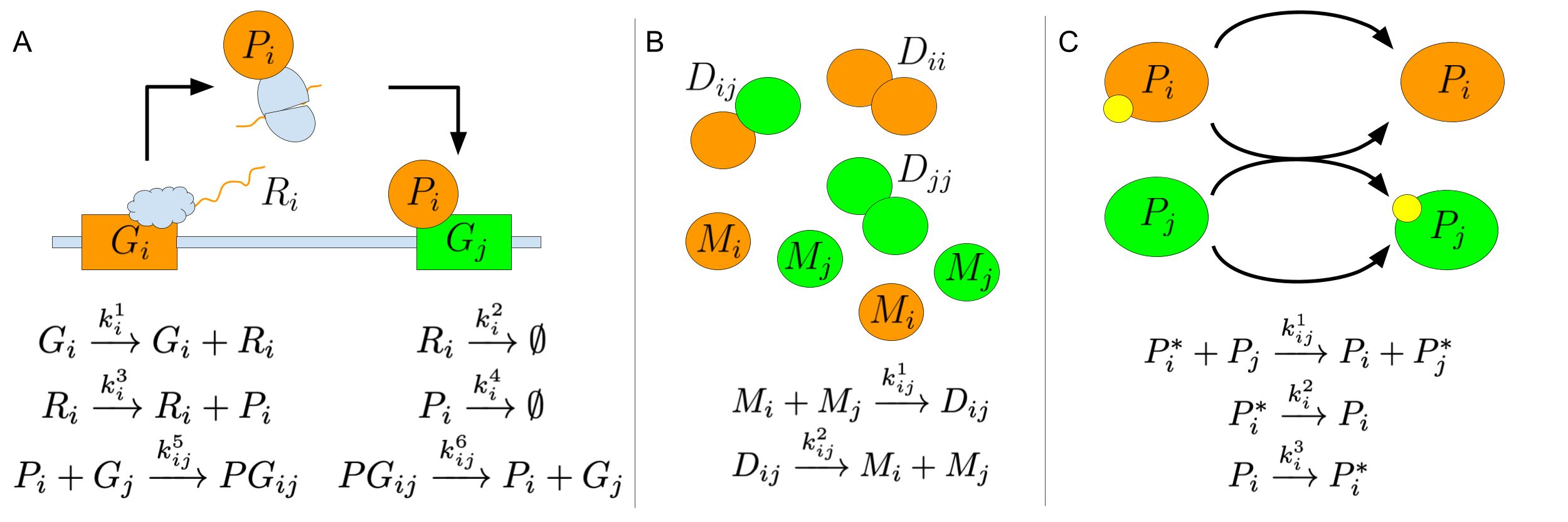
The starting point for our current work is to look for representations that reflect parallels between complex biochemical systems and neural networks. Canonical examples in biology include systems of metabolic enzymes [27], genetic regulatory networks [42, 7], signal transduction cascades [6, 14], and protein dimerization networks [48]. Inspired by these examples, synthetic biochemical systems have been explicitly designed to perform neural computation and experimentally demonstrated in cell-free enzyme systems [34, 35, 36, 24, 47], in DNA strand displacement cascades [51, 11, 64, 63, 67], and in living cells [52, 10]. The “neural” character of these systems stems from several factors: they have complex, multidimensional, nonlinear, analog dynamics that depend on a plethora of tunable parameters (such as reaction rate constants) and can perform information-processing tasks such as pattern recognition and attractor-based computation. Moreover, each type of network (e.g. metabolic, genetic regulation, signal transduction, dimerization) may be understood, in a simplified fashion, in terms of many instances of a prototypical mechanism, each differing only by its quantitative parameters – similar to how neural network models are often described in terms of a standard neural unit parameterized by weights and a threshold. Informally, we call such systems “index-amenable” because each species or reaction rate (or neuron or weight) can be identified by an index or tuple of indices; see Fig 1 for three examples based on genetic regulatory networks [7], dimerization networks [48], and phosphorelay networks [14, 9].
A particularly intriguing question is how biochemical “neural” computation can help make the decisions necessary to guide organismal development [42]. Reaction-diffusion systems, as pioneered by Alan Turing [62], provide a simplified model system – with local CRN dynamics spatially coupled by passive diffusion – for examining possible mechanisms for pattern formation. Even very simple CRNs can, in the reaction-diffusion context, give rise to complex textures and biological-looking patterns [49, 38]. Inspired by the neural cellular automaton model [45] that illustrated how a spatial array of neural networks can be trained to grow and maintain a precise “organismal” pattern, such as the image of a lizard, we have been exploring how a specific neural reaction-diffusion system can be trained for similar pattern formation tasks [8]. Both of these works employ differentiable programming techniques [16], where physical simulation models are optimized by automatic differentiation and gradient descent. Relevant to the work here, differentiable programming has been applied to small CRNs [44] as well as to complex cellular morphogenesis models [19].
The work reported here extends our prior work [8] by abstracting from a specific “neural” CRN to a general model for what we call indexed chemical reaction networks (ICRNs). ICRNs use index symbols to succinctly describe a set of species and reactions that can be naturally scaled to be arbitrarily large. Not only does indexing provide notational convenience, but the representation allows computations to be efficiently performed with tensors. Furthermore – and making a very pragmatic connection to neural computation – software utilizing tensors can leverage machine learning technologies to train parameters of the chemical system to optimize its behavior. A natural consequence of the ICRN representation is that species and reactions may involve more than one index, representing potential all-to-all interactions that some molecular biologists call “promiscuous” [1, 60] but that also correspond to what neuroscientists call “synaptic weights”. In neuroscience it is well understood that many weak interactions can dominate over select strong interactions in processes such as visual perception [56], highlighting the potential importance of even weak “promiscuous” interactions in molecular biology. We hope that the ICRN model can provide a natural framework for describing chemical systems that embody neural network principles of collective computation, thus helping facilitate the transfer of concepts, insights, mathematics, and software between fields.
2 Chemical Reaction Networks
The chemical reaction network (CRN) model is a general mathematical formalism for (typically) mass-action chemical kinetics described as ordinary differential equations (ODEs) [30]. Chemical reaction network theory, as presented by Feinberg [22], provides a canonical representation that models chemical systems with sets of objects: , , , . The set contains the species in consideration. For example, might be . The set of complexes are multisets of species, i.e., each complex assigns a count to each of the species. For example, is a complex. The set of reactions contains ordered pairs of complexes specifying the reactants and the products. For example, is a reaction.
Lastly, the rate constants are specified by a function that assigns a positive real number to a reaction. For example, if then we may write . A CRN is specified by the tuple .
In practice, Feinberg’s canonical representation is inconvenient for simulation software, where it may be desirable to allow reaction rate constants and to permit the same reaction to be listed multiple times, perhaps with different rate constants. The usual convention, which we take here, is to sum rate constants in that case, e.g., if a CRN contains and and , where , then this would correspond in Feinberg’s canonical representation to a single reaction with unless , in which case the reaction would not be included in .
A chemical state is given as , representing the concentrations of each species. The notation refers to -length tuples where each component corresponds to an element of and specifies a non-negative real number for that species. For complex , define , the product over species in a complex of each concentration raised to the power of the respective stoichiometric coefficient. (Here, we define to completely ignore species whose stoichiometry is zero.) Then the mass action chemical kinetics for canonical CRN or equivalent non-canonical CRN list , with possibly repeated reactions listed, can be described by the ODE
where the difference of complex multisets and is interpreted as a vector in , and .
3 Indexed Chemical Reaction Networks
The indexed chemical reaction network (ICRN) model provides an abstraction and representation suitable for the specification and simulation of index-amenable chemical systems. To specify an ICRN for simulation, one provides symbolic information akin to the descriptions in Fig 1 together with the ranges for indices, complemented with numerical information for rate constant tensors and initial concentration tensors. Thus, the symbolic information can be very compact. Of course, since an ICRN may use any number of indices, including none, in a trivial sense every classical CRN can be considered to be an ICRN, and in this case no efficiency improvement is obtained for the specification of the system. In the other direction, given an ICRN we can obtain a CRN by enumeration: replacing each indexed reaction by a finite set of concrete CRN reactions in which index symbols take on particular values. The dynamics for ICRNs are defined below so as to ensure that an ICRN and its enumerated CRN always give identical chemical kinetics.
ICRNs and CRNs are structurally similar, and so share terminology, such as species, reactions, and rate constants. Yet the two representations differ in that ICRN objects are the multidimensional analogs of CRN objects. When necessary, to avoid confusion, the term indexed will be used to describe objects of the ICRN and the term concrete will be used to describe objects of the underlying CRN.
3.1 Winner-Take-All ICRN
The winner-take-all DNA neural network from Cherry and Qian [11] is a prime example of a CRN with neural-network-like structure, and thus will be used both for illustrating the ICRN formalism here and for the first simulation and training example in Section 5. It can be described by the following indexed reactions.
In an indexed reaction, base species, such as , and base rate constants, such as are associated with index symbols, . Associating specific values to all the index symbols in an indexed reaction describes a concrete reaction. For example, assigning values and in the first indexed reaction gives the concrete reaction . The enumeration of the first indexed reaction is the collection of concrete reactions formed by substituting every combination of . The enumeration of the ICRN is the collection of enumerations for each of its indexed reactions. This enumeration is a multiset: the same reaction may appear multiple times, possibly with different rate constants, and in such cases the effective rates constants are summed.
3.2 ICRN Definitions
By discussing ICRNs as representations of chemical systems, we have considered meaning, or semantics. Turning our attention to syntax, what are the rules for constructing ICRNs? The reader should pause and consider whether the examples below are valid ICRNs ().
We will define the ICRN, covering its syntax and its relationship to its semantics. Just as the various CRN conventions can be understood in terms of Feinberg’s formalism, our formalism serves as a common way to precisely describe ICRNs.
An ICRN is specified by five collections: . The base species and base rate constants are multidimensional analogs of species and rate constants from concrete CRNs. Indexed reactions use index symbols to describe interactions between the multidimensional objects. The index sets describe the index values that are valid to associate with base species, base rate constants, or indexed reactions.
Index symbols are essential for the abstraction provided by ICRNs. In the winner-take-all system, the set of index symbols contains index symbols . Each index symbol has an associated index set, denoted , which is the set of values the index symbol can take on. For example, . A tuple of index symbols has an index set that is the product of the index sets of its constituent index symbols .
Defining index symbols as objects that exist globally throughout the system, as opposed to each indexed reaction having its own notion of index symbols, has two advantages. Firstly, global index symbols avoid the confusion that arises when the same index symbol appears in multiple reactions but takes on different values across the reactions. Secondly, global index symbols directly represent entities of the system. In the winner-take-all system, there are inputs and outputs to a winner-take-all computation. Thus, the index symbol represents a single input while and are used to represent a single output.
Base species and base rate constants are multidimensional objects representing groups of concrete species and concrete rate constants, respectively. Both base species and base rate constants have index sets, denoted for base species and for base rate constants . A base species maps from its index set to a concrete species, while a base rate constant maps from its index set to a concrete rate constant. For example, the base species has an index set and represents a group of concrete species, . Base species can be thought of as dictating the overall structure of a group of biomolecules that vary at designated regions, or domains. Each concrete species is a specific variation of the overall structure and specifies the chemical identity of the domains.
Fixing , , and , and their index sets, there is a notion of a set of valid indexed species and a set of valid indexed rate constants . An indexed object is valid if the index set of the base object and index set of the index symbols are the same.
An indexed reaction is a triple in . Reactants and products are multisets of and are accompanied by an indexed rate constant from . The set of index symbols present in the indexed reaction implies the index set of the indexed reaction, denoted . Specifying values for each index symbol specifies a concrete reaction, so indexed reactions are functions from the index set to concrete reactions. The enumeration of an indexed reaction is the image of the index set under , . The enumeration of an ICRN is the multiset union of the enumeration of each indexed reaction: .
At this point, the reader should be able to identify as the ill-defined ICRN. The other three ICRNs are valid given that the index sets of their objects are in agreement. Additionally, the reader may have noticed indexed species written as rather than . For instance, we wrote instead of . The former notation emphasizes the concrete object that results from enumeration. However, indexed bases and indexed rate constants are objects in their own right and are, strictly speaking, the building blocks of indexed reactions. When there is room for confusion, the latter notation will be used to refer to indexed species and indexed rate constants.
ICRNs can be enumerated to capture a wide variety of concrete CRNs. There are systems of interest that are well suited to being described by indexed reactions but with restricted index sets. In many of these cases, the system of interest can be captured by creative use of the base species and base rate constants. For example, in the winner-take-all system, the implementation of the annihilation reaction in the DNA substrate produces a non-functioning annihilator molecule for the case where . This restriction in indexing can be addressed by setting when , so the concrete reaction does not occur for . Symmetric systems in particular are discussed further in appendix A.
3.3 Dynamics
The dynamics of an ICRN follows the dynamics of the enumerated CRN. Concentrations of base species and base rate constants are naturally represented as tensors. Accordingly, the dynamics of an ICRN can be expressed with tensor operations, which can be derived through symbolic manipulation of the ICRN.
The tensor representing the concentrations for base species is written as , where with . To distinguish between the concentrations associated with the ICRN and the concrete CRN that it abstracts, we will use to refer to concentrations in the ICRN representation and to refer to the concentration of the concrete species, , where . The time-dependent state of an ICRN is where . Thus, specifies for all . The dynamics of an ICRN describes the time derivative of , which is the tuple of time derivatives for each :
The dynamics for the ICRN follows the dynamics of the enumerated concrete CRN, so the time derivative for is the collection of time derivatives for each concrete species represented by , where the time derivative of is defined by the time derivative of from the enumerated concrete CRN:
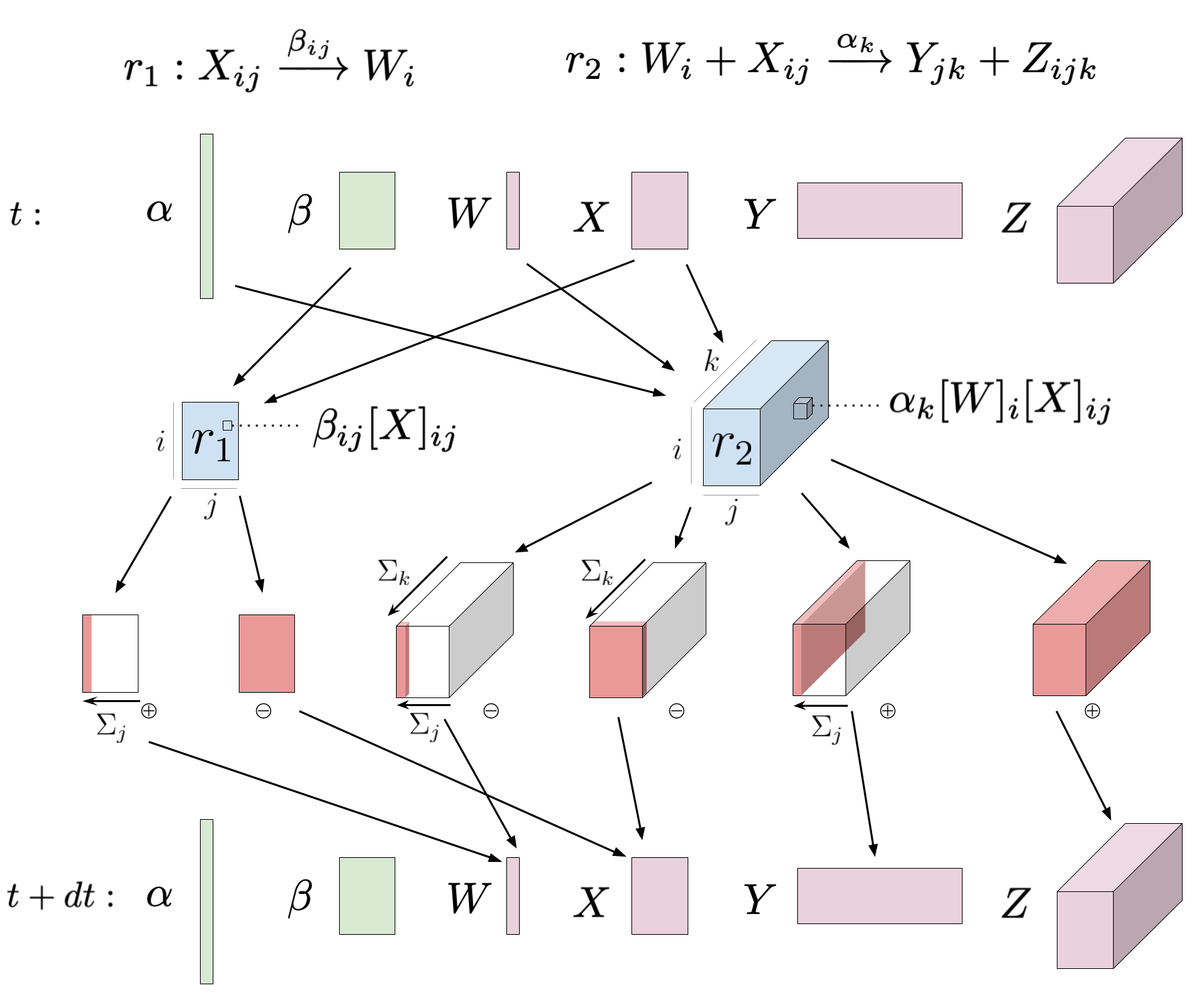
As seen in Fig 2, each indexed reaction has an associated indexed reaction flux , a real-valued tensor. For each appearance of an indexed species , sums are taken along the dimensions of that correspond to index symbols that are present in the indexed reaction but not present in the indexed species. The result is the flux contribution to , denoted , which is a real-valued tensor with the same shape as . A base species receives contributions from every appearance of any indexed species that derives from among all the indexed reactions.
The indexed reaction flux, is a real-valued tensor with the same shape as the index set of . Let be index symbols such that and be the multisets of reactants and products, respectively. Then , where is an indexed species. Additionally, let be the indexed rate constant used in reaction . Here, is the real-valued rate constant. The following is an element-wise specification of , indexing with , since all index symbols in are present in the right hand expression.
The flux contribution to from depends on which indexed species is participating in the reaction. The following equation is an element-wise specification of the tensor using the index symbols .
On the right hand side, is the tuple of index symbols in and refers to the index symbols that are in but not . Thus, the right hand side is an expression that is parameterized by . Moreover, the summation is an Einstein summation, a kind of indexed summation which can be efficiently computed [58].
The totality of the contributions to from each appearance of a derived indexed species can be formulated as the following element-wise specification.
The left hand side describes the rate of change of an element of corresponding to index symbols . On the right, refers to an element of the tensor indexed by . Since , the right hand side is an expression parameterized by . An example of the dynamics derivation appears in appendix B.
ICRNs can be extended naturally from the well-mixed to a spatial setting, becoming reaction-diffusion systems. For classical CRNs, reaction-diffusion dynamics are described mathematically by a PDE: . For reaction-diffusion with species in spatial dimensions, the concentration field is a function , with a bounded subset of the spatial dimension. is a diagonal matrix of diffusion constants, is the Laplacian operator encoding diffusion, and represents the derivatives due to the CRN’s reactions. ICRNs require only a tensor generalization of these semantics.
4 Software
The icrn Python library allows for efficient simulation and training of ICRNs by compiling a general ICRN into its dynamics in a tensor-based and differentiable framework. The SymPy symbolic programming library [41] is used for transforming an ICRN representation into a function that computes the dynamics and influenced the nomenclature of the ICRN definitions. While the ICRN representation is symbolic, the dynamics function is numerical and takes as input real-valued tensors for concentrations and rate constant information to compute a change of concentrations. In the icrn library, tensors and the operations between them are backed by JAX [5], so the dynamics computation is not only efficient, making use of hardware acceleration to speed up tensor computations, but also is automatically differentiable, allowing for gradient based optimization methods.
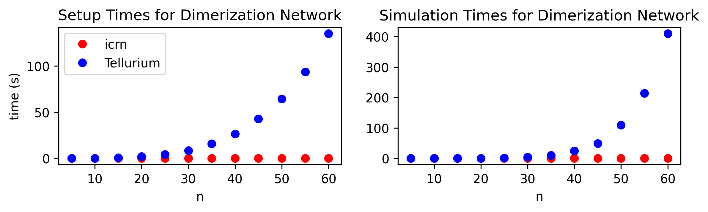
Existing reaction system simulators, such as Tellurium [12], do not take advantage of mapping of dynamics onto tensor operations. Fig 3 compares the use of the icrn library and Tellurium for setting up and simulating dimerization networks from Fig 1 with varying , the number of monomer species.
Well-mixed systems are simulated explicitly using forwards Euler or Runge-Kutta methods adapted to tensor operations. As of writing, icrn has only limited support for time-scale separation: “fast” reactions that go to completion (not equilibrium or steady-state) within each time step, subject to the restriction that no species may appear as a reactant in more than one fast reaction. To simulate reaction diffusion, we use a finite-differences numerical scheme, dividing both the spatial and temporal dimensions into discrete points, and deriving operators for the reaction and diffusion update steps. Thus, spatial extent expands the dimensions of concentration tensors, with discretized positions playing a role analogous to indices. Our ICRN simulator software uses an implicit-explicit (IMEX) integration scheme: diffusion derivatives are solved implicitly in the Fourier domain [54], and the reaction derivatives are handled explicitly. The icrn package and notebooks with code for the examples below are available at https://github.com/SwissChardLeaf/icrn.
5 Examples
We provide three examples, demonstrating different aspects of the ICRN formalism and our icrn software. First, we simulate the winner-take-all example described earlier, showing that the starting concentrations may be optimized by gradient descent to perform the classification task, rather than set manually as in [11]. Second, we explore the Gray-Scott reaction-diffusion model [25]. While this is a simple CRN and does not stand to gain from indexing, it serves to illustrate how tensor-based simulation facilitates reaction-diffusion modeling and how differential programming can be used to find parameters that produce target textures. Finally, we replicate the developmental pattern formation task from [8], showing how icrn can be used to efficiently optimize a large (256 species) ICRN in the reaction-diffusion setting.
5.1 Indexed Well Mixed – Winner-Take-All
.png)
The abstract winner-take-all computation can classify hand written digits. Following Cherry and Qian [11], our dataset is a reduced-resolution subset of the MNIST [18] dataset and consists of input-output pairs where indicates a specific pair, specifies a by image of a handwritten digit, and specifies the digit that the image represents (seven, eight, or nine). A digit classifier is a function from images to classes. The abstract winner-take-all computation acts as a classifier by computing weighted sums for each class and taking the class with the highest sum to be the output class. The weights are specified by a matrix , where a column contains the weights used in the weighted sum per class.
Cherry and Qian set the weights of the classifier by pruning an average-digit matrix. Average-digit weights are the averages of examples in the training data. A column of the weight matrix is populated by the average of from the digit class corresponding to the column. Due to experimental limitations from having many nonzero elements, the pruned matrix takes the highest elements of each class.
The winner-take-all ICRN can be trained to optimize different qualities. One view is that the fluorescence signal for the correct class should completely saturate (at 100 nM) while for other classes it is . A large difference in the output fluorescence is important experimentally for being able to resolve the output signal from the classifier. The superiority score captures this idea, for a given target input-output pair that results in endpoint fluorescence vector . Ideal behavior gives a superiority metric of , and lower values reflect deviation from the ideal (Fig 4B). The loss function can be set to produce a weight matrix with a high superiority metric. Another possibility is to optimize the ICRN’s ability to produce the correct output without a concern for how low the fluorescence is for the other output classes. The endpoint fluorescence can be interpreted as a probability by normalizing with the softmax function, . The loss function computes a cross entropy loss with an regularization term, , that penalizes high weights, which encourages the training process to produce fewer nonzero weights, increasing experimental feasibility. The results of applying these training methods are shown in Fig 4D.
5.2 Reaction Diffusion – Gray-Scott Textures
We will begin with the Gray-Scott model [25] to illustrate the simulation and training of reaction-diffusion systems within our software framework. The Gray-Scott model is a reaction-diffusion system with just two species, and , and four reactions: , , , and . As such, it does not stand to gain simplicity from indexing, but nonetheless it is a (trivial) instance of an ICRN. The PDE can be written as:
This reaction-diffusion system has just four parameters: rate constants and , and diffusion constants and . However, tuning these parameters, the system generates a wide variety of patterns, both stable and time-varying, explored and categorized by Pearson [49].
Our task is to use differentiable programming [16] to find Gray-Scott parameters that yield a particular type of pattern – e.g. mazes, spots, waves. As in Pearson’s paper, we will fix the diffusion constants (with diffusing twice as fast as ), and vary only and . We set up the task as follows: first, we choose and to yield a certain type of pattern when simulated forwards from initial conditions randomly sampled from a distribution (see Fig 5). The Gray-Scott PDE is fairly stiff, necessitating many steps with small to let its characteristic patterns develop from unstructured initial conditions. We thus take a single long simulation output using these parameters, and call this our target pattern. During training, we will run shorter simulations that are more amenable to gradient descent, but which will introduce other challenges.
.png)
Next, we need to define a loss function measuring how closely simulations during training match the target. We would like the loss function to be relatively stable to different initial conditions, so we cannot use a simple pixel-by-pixel comparison of simulation output and target: rather, we want something that captures and compares the qualitative features of the patterns. Taking inspiration from work on neural transfer of artistic style [23] and matching textures with self-organizing neural cellular automata [43], we evaluate pattern matches using the low-level (early layer) features from VGG-16, a convolutional neural network trained for image classification [57]. We feed our target pattern to VGG-16 as an input, and extract the activations from the first through third max-pooling layers. We then compute Gram matrices from these features, capturing some sense of how different elements of the pattern vary with each other over space. The Gram matrix element , where and are the spatial dimensions of the layer and is feature at position in layer .
Finally, we can compute a stylistic loss function, defined as the mean squared distance between the target Gram matrices and those extracted from the simulated output by the same process: . For stability, we augment the loss by adding a “moments-matching” term, comparing the means and log-variances of the simulation outputs with reference values, drawn by simulating the Gray-Scott model in different parts of the pattern-forming parameter space:
Here, is the simulated output, and is an average over ten reference simulation outputs, and is the variance of . Finally, we add a “potential well” regularization term, penalizing parameter values outside of the pattern-forming region of We then have loss .
We train the parameters using gradient descent on this loss function applied to the output of short simulations that start with the target pattern rather than a random noise state. Thus we are accommodating the stiffness of the Gray-Scott PDE by training for stability rather than for de novo generation of the texture. This has an additional benefit in that for some parameters, pattern formation in the Gray-Scott system can fail to “kick start” properly for random initial conditions. As in the winner-take-all example, both the simulation (using icrn) and loss function computation are written using differentiable JAX primitives, meaning that the derivatives may be calculated automatically using backpropagation-through-time (BPTT) [2, 53]. We integrate the gradients using mini-batch gradient descent, adding a small amount of randomness to the parameters when the learning converges to a local minimum.
The results shown in Fig 5, including a final long simulation from the lowest loss endpoint among the training runs, are perhaps deceptively well-behaved: training of this system was finicky and challenging. The vast bulk of parameter combinations give rise to spatially homogeneous outputs, and only in a sliver of parameter space are interesting patterns to be found – and there, the sensitivity to initial state was often confounding. Making this problem even harder, learning can turn just two knobs, and . The success of modern machine learning in many contexts is thanks to, among other things, the high dimensionality of deep neural networks. With so many parameters, there is almost always some direction in parameter space we can move along to reduce the loss, meaning that even simple, first-order optimization algorithms like gradient descent perform well. In the next section we will consider an ICRN with tens of thousands of parameters in the reaction-diffusion setting. Though small by modern standards, it is big enough to enjoy the blessings of dimensionality.
5.3 Indexed Reaction Diffusion – Hopfield CRN Images
Reaction-diffusion systems can be trained to grow into significantly more complex patterns. Here, we take the Hopfield network-inspired CRN and training approach used in [8], and train an ICRN to grow from simple initial conditions into a rendering of a photograph.
The Hopfield CRN consists of a set of neurons , with variables , and for an -neuron system. In the well-mixed setting, the Hopfield CRN can be trained to store a set of “memories”, similar to the classical Hopfield network [29]. The neurons are connected all-to-all. Catalytic reactions between pairs of neurons correspond to weighted sums, and a trimolecular degradation reaction for each neuron corresponds to an activation function. To allow negative values for the variables, and negative weights between neurons, we use a dual-rail representation: the variable is the difference in the concentrations of two species, , with . A fast annihilation reaction is added between the positive and negative species for each variable. The ICRN is defined as
| Weighted sums: | Degradation: | ||
| Annihilation: | |||
where , ensuring that all rate constants are non-negative. The parameters for the Hopfield ICRN consist of two weight matrices and (with ), two -vectors of degradation rate constants and (with ), and two -vectors of diffusion constants and (with ). When the weight matrices are symmetric and degradation rate constants are equal, the Hopfield ICRN has equivalent attractor-basin structure as the classical Hopfield associative memory, but we find that allowing asymmetric and unequal parameters facilitates improved pattern formation [8]. The ICRN software admits an efficient representation of dual-rail ICRNs.
The training approach and loss function for the pattern forming task was inspired by Mordvintsev’s work on neural cellular automata [45]. We define the first three variables () to be the visible units, corresponding to red, green, and blue, and the remaining are hidden. We pick an RGB target image , and train the parameters of the ICRN such that the visible state of the system matches the target as closely as possible, when it is grown from specified initial conditions for a specific duration of time, . The target in Fig 6 is grayscale, but we treat it in RGB for generality. We can write the pixel-wise loss as
where and are the discretized points in space. The loss function considers only the visible species. This loss is simpler than that used in the Gray-Scott example, but is also less flexible – a pattern which to the eye appears similar in style may have a high loss, if the pixel values are different. As in the Gray-Scott training task, we train the rate constants, but for this task we also train the diffusion constants. Unlike in the winner-take-all example, the initial conditions are fixed, consisting of a simple asymmetric pattern in the visible units. We use the Optax implementation of the Adam optimizer [37, 17].
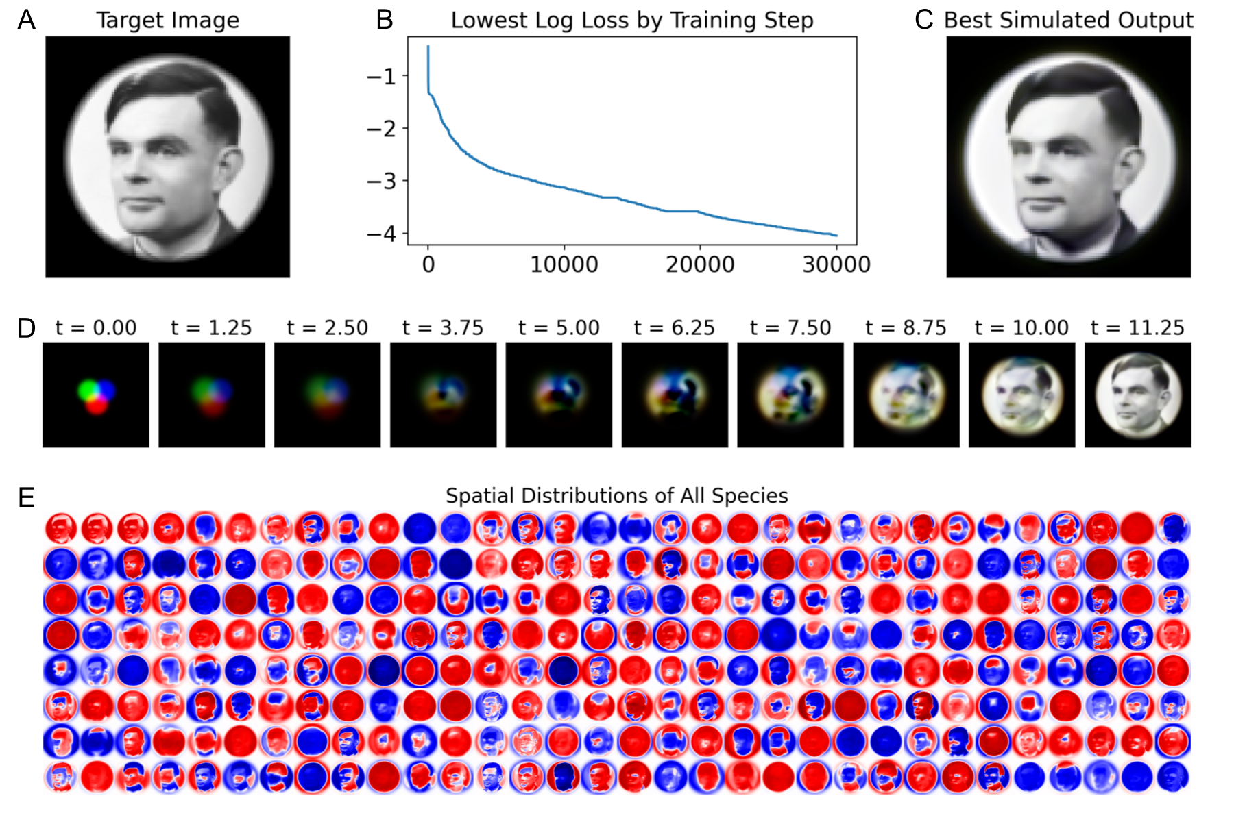
Fig 6 shows the training of a Hopfield ICRN with neurons. The corresponding CRN has 512 species (two per dual-rail variable), 131072 () catalytic rate constants, 512 () degradation rate constants, and 512 () diffusion constants, all of which may be varied during training. This amounts to considerably more real values than the grayscale pixels of the target image, helping explain the accuracy of pattern formation. In general, we observe that increasing allows the training procedure to find a set of parameters with a lower loss.
The Hopfield CRN has several other notable differences from the Gray-Scott model. First, it is much less sensitive to how the parameters are initialized, and the choice of target pattern. Most training runs are at least somewhat successful, matching the target to some level of fidelity. Second, the Hopfield reaction-diffusion system is less stiff, and so can grow into the pattern in fewer steps without encountering numerical errors. With so many species, the state of the system occupies significant memory, and so we use gradient checkpointing to reduce the memory overheads from backpropagation-through-time [26]. Finally, note that the target image is a correct snapshot at the specified time, but is not stable – more sophisticated training procedures are discussed in [8] that improve the stability and robustness of pattern formation in Hopfield CRNs.
6 Discussion
We have demonstrated that the dynamics of ICRNs can be expressed and computed efficiently for systems with mass action kinetics. At this point the reader may be asking themselves whether there is a general principle for when a CRN is index-amenable and would benefit from the ICRN representation. We know of no concise characterization, and indeed the choice depends upon how simple the rate constant tensors can be. For example, any CRN involving only count-preserving bimolecular reactions can be represented as an ICRN with just one indexed reaction, , together with a perhaps very sparse 4-dimensional tensor for . A framework like this was the starting point for the prior differentiable programming of small CRNs [44]. The optimal tradeoff for the number of indexed reactions and the complexity of the rate constant tensors may be quite subtle.
Toward the goal of concise representations, observe that rate laws other than mass action as well as a variety of timescale separation conventions are used widely because they allow for simplifying assumptions, such as general pseudo-steady-state approximations, that result in more compact CRNs. For example, in systems with an enzyme concentration sufficiently lower than the substrate concentration, utilizing Michaelis-Menten kinetics allows the simulation to disregard the enzyme concentration. Appropriate formalisms and compilation methods that will produce efficient tensor operations for these cases have yet to be developed.
Once ICRNs are compiled into dynamics expressed through tensor operations, there are a variety of numerical methods for forward simulation of ICRNs, and choosing among these options is particularly important for the training of ICRNs. Simple integration methods often perform poorly on stiff problems, requiring small and multiple time steps, which has two significant consequences for training the ICRN. Firstly, an increase in simulation steps increases the memory requirements during backpropagation, limiting the size of ICRN that can be trained. Secondly, the learning algorithm may enter a region of the state space with low loss but with numerical artifacts. In these cases, the learned weights are invalid as the simulation no longer reflects the time evolution of the physical system. Expanding support for more sophisticated numerical methods will open doors for training stiff ICRNs.
All the ICRNs in the examples were trained by evaluating loss against a target state at the end of simulation. However, the target could be a trajectory through time and the loss could be evaluated over multiple time points. Others have trained parameters of chemical systems to fit trajectories but consider a restricted class of CRNs [44, 15]. On the other hand, our work considers the training of ICRNs with no restriction. One advantage of this flexibility is the increased potential to train experimental systems. If an experimental system can be written as an ICRN, and data regarding the target behavior can be gathered, the ICRN can be trained to perform the target behavior. Of course, there is no guarantee that the ICRN will respond well to training. The value of the ICRN formalism and software is precisely to uncover the classes of ICRNs that respond well.
DNA is especially well-suited as a molecular substrate to physically realize large ICRNs designed in this way. The biophysics of DNA-DNA interactions are relatively well-understood and modeled, and are simple enough that they can sometimes be abstracted without a critical loss of detail. Tools like NUPACK [68] enable the design of large libraries of sequences which are more or less orthogonal, enabling the creation of standardized components that can be scaled to large systems without too much cross-talk. The Hopfield CRN relies on non-orthogonal interactions (“promiscuous”, quadratic with the number of neurons), and progress has been made on tools to design DNA molecules with a range of non-orthogonal interactions [46, 3]. Prior work has also shown a theoretical basis for the morphogenesis of arbitrary patterns in reaction-diffusion systems [55], although using a digital circuits-inspired approach which may be hard to scale to more complex patterns. On the experimental side, nucleic acids have been used to generate reaction-diffusion patterns in a wide range of approaches, as reviewed in [65]. Though the pattern-forming Hopfield CRN has not been implemented experimentally, we believe it is at least on the horizon of feasibility in DNA.
The abstraction of DNA design is not yet at the level of silicon and transistors, but is much more straightforward than the design of proteins or organic molecules. These molecules have much more complex dynamics, and in general systems built with them face the problem that parameters cannot be changed independently of each other: changing a protein’s fold will affect how it interacts with all other proteins. Impressive work has been done in synthetic biology, including the synthetic morphogenesis of bacterial colonies [20] and mammalian cells [61]. Still, these patterns are closer in their complexity to those formed by simple reaction-diffusion systems like Gray-Scott. As tools for biomolecular design continue to improve – think of protein design models like AlphaFold [33] and RFdiffusion [66] – it is interesting to consider what sorts of biological design tasks will become possible.
Some biological and computational systems can also learn autonomously. This is clearly the case for humans, but even relatively simple CRNs (e.g. for linear regression) can be designed to do gradient descent on a chemically-specified loss function, learning a representation via their dynamics, rather than externally [39, 50]. Homo sapiens slowly changes from one generation to the next under evolution, but individual humans also learn from their experiences. This relationship can be thought of in the frame of inner-vs-outer optimization [13], or meta-learning [31]. It is thought-provoking to consider how CRNs could be designed to autonomously learn to execute more complex tasks, like pattern formation.
References
- [1] Amir Aharoni, Leonid Gaidukov, Olga Khersonsky, Stephen McQ Gould, Cintia Roodveldt, and Dan S. Tawfik. The “evolvability” of promiscuous protein functions. Nature Genetics, 37:73–76, 2005.
- [2] Atılım Günes Baydin, Barak A. Pearlmutter, Alexey Andreyevich Radul, and Jeffrey Mark Siskind. Automatic differentiation in machine learning: a survey. J. Mach. Learn. Res., 18:5595–5637, 2017.
- [3] Joseph Don Berleant. Rational design of DNA sequences with non-orthogonal binding interactions. In International Conference on DNA Computing and Molecular Programming, pages 4:1–4:22, 2023. doi:10.4230/LIPICS.DNA.29.4.
- [4] Pierre Boutillier, Mutaamba Maasha, Xing Li, Héctor F. Medina-Abarca, Jean Krivine, Jérôme Feret, Ioana Cristescu, Angus G. Forbes, and Walter Fontana. The Kappa platform for rule-based modeling. Bioinformatics, 34:i583–i592, 2018. doi:10.1093/BIOINFORMATICS/BTY272.
- [5] James Bradbury, Roy Frostig, Peter Hawkins, Matthew James Johnson, Chris Leary, Dougal Maclaurin, George Necula, Adam Paszke, Jake VanderPlas, Skye Wanderman-Milne, and Qiao Zhang. JAX: composable transformations of Python+NumPy programs, 2018. URL: http://github.com/jax-ml/jax.
- [6] Dennis Bray. Protein molecules as computational elements in living cells. Nature, 376:307–312, 1995.
- [7] Nicolas E. Buchler, Ulrich Gerland, and Terence Hwa. On schemes of combinatorial transcription logic. Proceedings of the National Academy of Sciences, 100:5136–5141, 2003.
- [8] Salvador Buse and Erik Winfree. Developmental pattern formation in neural reaction-diffusion systems. Manuscript in preparation, 2025.
- [9] Chun-Hsiang Chan, Cheng-Yu Shih, and Ho-Lin Chen. On the computational power of phosphate transfer reaction networks. New Generation Computing, 40:603–621, 2022. doi:10.1007/S00354-022-00154-6.
- [10] Zibo Chen, James M. Linton, Shiyu Xia, Xinwen Fan, Dingchen Yu, Jinglin Wang, Ronghui Zhu, and Michael B. Elowitz. A synthetic protein-level neural network in mammalian cells. Science, 386:1243–1250, 2024.
- [11] Kevin M. Cherry and Lulu Qian. Scaling up molecular pattern recognition with DNA-based winner-take-all neural networks. Nature, 559:370–376, 2018.
- [12] Kiri Choi, J. Kyle Medley, Matthias König, Kaylene Stocking, Lucian Smith, Stanley Gu, and Herbert M. Sauro. Tellurium: an extensible Python-based modeling environment for systems and synthetic biology. Biosystems, 171:74–79, 2018. doi:10.1016/J.BIOSYSTEMS.2018.07.006.
- [13] Benoít Colson, Patrice Marcotte, and Gilles Savard. Bilevel programming: A survey. 4OR, 3:87–107, 2005. doi:10.1007/S10288-005-0071-0.
- [14] Attila Csikász-Nagy, Luca Cardelli, and Orkun S. Soyer. Response dynamics of phosphorelays suggest their potential utility in cell signalling. Journal of The Royal Society Interface, 8:480–488, 2011.
- [15] Alexander Dack, Benjamin Qureshi, Thomas E. Ouldridge, and Tomislav Plesa. Recurrent neural chemical reaction networks that approximate arbitrary dynamics, 2024. arXiv:2406.03456.
- [16] Filipe de Avila Belbute-Peres, Kevin Smith, Kelsey Allen, Josh Tenenbaum, and J. Zico Kolter. End-to-end differentiable physics for learning and control. In Advances in Neural Information Processing Systems, volume 31, pages 7178–7189, 2018. URL: https://proceedings.neurips.cc/paper/2018/hash/842424a1d0595b76ec4fa03c46e8d755-Abstract.html.
- [17] DeepMind, Igor Babuschkin, Kate Baumli, Alison Bell, Surya Bhupatiraju, Jake Bruce, Peter Buchlovsky, David Budden, Trevor Cai, Aidan Clark, Ivo Danihelka, Antoine Dedieu, Claudio Fantacci, Jonathan Godwin, Chris Jones, Ross Hemsley, Tom Hennigan, Matteo Hessel, Shaobo Hou, Steven Kapturowski, Thomas Keck, Iurii Kemaev, Michael King, Markus Kunesch, Lena Martens, Hamza Merzic, Vladimir Mikulik, Tamara Norman, George Papamakarios, John Quan, Roman Ring, Francisco Ruiz, Alvaro Sanchez, Laurent Sartran, Rosalia Schneider, Eren Sezener, Stephen Spencer, Srivatsan Srinivasan, Miloš Stanojević, Wojciech Stokowiec, Luyu Wang, Guangyao Zhou, and Fabio Viola. The DeepMind JAX Ecosystem, 2020. URL: http://github.com/google-deepmind.
- [18] Li Deng. The MNIST database of handwritten digit images for machine learning research. IEEE Signal Processing Magazine, 29:141–142, 2012. doi:10.1109/MSP.2012.2211477.
- [19] Ramya Deshpande, Francesco Mottes, Ariana-Dalia Vlad, Michael P. Brenner, and Alma Dal Co. Engineering morphogenesis of cell clusters with differentiable programming, 2024. doi:10.48550/arXiv.2407.06295.
- [20] Salva Duran-Nebreda, Jordi Pla, Blai Vidiella, Jordi Piñero, Nuria Conde-Pueyo, and Ricard Solé. Synthetic lateral inhibition in periodic pattern forming microbial colonies. ACS Synthetic Biology, 10:277–285, 2021.
- [21] Irving R. Epstein and John A. Pojman. An Introduction to Nonlinear Chemical Dynamics: Oscillations, Waves, Patterns, and Chaos. Oxford University Press, 1998.
- [22] Martin Feinberg. Foundations of Chemical Reaction Network Theory. Springer International Publishing, 2019.
- [23] Leon A. Gatys, Alexander S. Ecker, and Matthias Bethge. Image style transfer using convolutional neural networks. In Proceedings of the IEEE Conference on Computer Vision and Pattern Recognition (CVPR), pages 2414–2423, 2016. doi:10.1109/CVPR.2016.265.
- [24] Anthony J. Genot, Teruo Fujii, and Yannick Rondelez. Scaling down DNA circuits with competitive neural networks. Journal of The Royal Society Interface, 10:20130212, 2013.
- [25] Peter Gray and Stephen K. Scott. Autocatalytic reactions in the isothermal, continuous stirred tank reactor: Oscillations and instabilities in the system A + 2B → 3B; B → C. Chemical Engineering Science, 39:1087–1097, 1984.
- [26] Andreas Griewank and Andrea Walther. Revolve: An implementation of checkpointing for the reverse or adjoint mode of computational differentiation. ACM Transactions on Mathematical Software, 26:19–45, 2000.
- [27] Allen Hjelmfelt, Edward D. Weinberger, and John Ross. Chemical implementation of neural networks and Turing machines. Proceedings of the National Academy of Sciences, 88:10983–10987, 1991.
- [28] Stefan Hoops, Sven Sahle, Ralph Gauges, Christine Lee, Jürgen Pahle, Natalia Simus, Mudita Singhal, Liang Xu, Pedro Mendes, and Ursula Kummer. COPASI—a complex pathway simulator. Bioinformatics, 22:3067–3074, 2006. doi:10.1093/BIOINFORMATICS/BTL485.
- [29] John J. Hopfield. Neural networks and physical systems with emergent collective computational abilities. Proceedings of the National Academy of Sciences, 79:2554–2558, 1982.
- [30] Fritz Horn and Roy Jackson. General mass action kinetics. Archive for Rational Mechanics and Analysis, 47:81–116, 1972.
- [31] Timothy Hospedales, Antreas Antoniou, Paul Micaelli, and Amos Storkey. Meta-learning in neural networks: A survey. IEEE Transactions on Pattern Analysis and Machine Intelligence, 44:5149–5169, 2021. doi:10.1109/TPAMI.2021.3079209.
- [32] Michael Hucka, Andrew Finney, Herbert M. Sauro, Hamid Bolouri, John C. Doyle, Hiroaki Kitano, Adam P. Arkin, Benjamin J. Bornstein, Dennis Bray, Athel Cornish-Bowden, et al. The systems biology markup language (SBML): a medium for representation and exchange of biochemical network models. Bioinformatics, 19:524–531, 2003. doi:10.1093/BIOINFORMATICS/BTG015.
- [33] John Jumper, Richard Evans, Alexander Pritzel, Tim Green, Michael Figurnov, Olaf Ronneberger, Kathryn Tunyasuvunakool, Russ Bates, Augustin Žídek, Anna Potapenko, Alex Bridgland, Clemens Meyer, Simon A. A. Kohl, Andrew J. Ballard, Andrew Cowie, Bernardino Romera-Paredes, Stanislav Nikolov, Rishub Jain, Jonas Adler, Trevor Back, Stig Petersen, David Reiman, Ellen Clancy, Michal Zielinski, Martin Steinegger, Michalina Pacholska, Tamas Berghammer, Sebastian Bodenstein, David Silver, Oriol Vinyals, Andrew W. Senior, Koray Kavukcuoglu, Pushmeet Kohli, and Demis Hassabis. Highly accurate protein structure prediction with AlphaFold. Nature, 596:583–589, 2021. doi:10.1038/s41586-021-03819-2.
- [34] Jongmin Kim, John Hopfield, and Erik Winfree. Neural network computation by in vitro transcriptional circuits. Advances in Neural Information Processing Systems, 17:681–688, 2004. URL: https://proceedings.neurips.cc/paper/2004/hash/65f2a94c8c2d56d5b43a1a3d9d811102-Abstract.html.
- [35] Jongmin Kim, Kristin S. White, and Erik Winfree. Construction of an in vitro bistable circuit from synthetic transcriptional switches. Molecular Systems Biology, 2:68, 2006.
- [36] Jongmin Kim and Erik Winfree. Synthetic in vitro transcriptional oscillators. Molecular Systems Biology, 7:465, 2011.
- [37] Diederik P. Kingma and Jimmy Ba. Adam: A method for stochastic optimization. In International Conference on Learning Representations, 2015. arXiv:1412.6980.
- [38] Shigeru Kondo and Takashi Miura. Reaction-diffusion model as a framework for understanding biological pattern formation. Science, 329:1616–1620, 2010.
- [39] Matthew R. Lakin. Design and simulation of a multilayer chemical neural network that learns via backpropagation. Artificial Life, 29:308–335, 2023. doi:10.1162/artl_a_00405.
- [40] Rahuman S. Malik-Sheriff, Mihai Glont, Tung VN Nguyen, Krishna Tiwari, Matthew G Roberts, Ashley Xavier, Manh T. Vu, Jinghao Men, Matthieu Maire, Sarubini Kananathan, et al. Biomodels—15 years of sharing computational models in life science. Nucleic acids research, 48:D407–D415, 2020. doi:10.1093/NAR/GKZ1055.
- [41] Aaron Meurer, Christopher P. Smith, Mateusz Paprocki, Ondřej Čertík, Sergey B. Kirpichev, Matthew Rocklin, Amit Kumar, Sergiu Ivanov, Jason K. Moore, Sartaj Singh, Thilina Rathnayake, Sean Vig, Brian E. Granger, Richard P. Muller, Francesco Bonazzi, Harsh Gupta, Shivam Vats, Fredrik Johansson, Fabian Pedregosa, Matthew J. Curry, Andy R. Terrel, Štěpán Roučka, Ashutosh Saboo, Isuru Fernando, Sumith Kulal, Robert Cimrman, and Anthony Scopatz. SymPy: symbolic computing in Python. PeerJ Computer Science, 3:e103, 2017. doi:10.7717/PEERJ-CS.103.
- [42] Eric Mjolsness, David H. Sharp, and John Reinitz. A connectionist model of development. Journal of Theoretical Biology, 152:429–453, 1991.
- [43] Alexander Mordvintsev, Eyvind Niklasson, and Ettore Randazzo. Texture generation with neural cellular automata, 2021. AI for Content Creation Workshop (CVPR). arXiv:2105.07299.
- [44] Alexander Mordvintsev, Ettore Randazzo, and Eyvind Niklasson. Differentiable programming of chemical reaction networks, 2023. doi:10.48550/arXiv.2302.02714.
- [45] Alexander Mordvintsev, Ettore Randazzo, Eyvind Niklasson, and Michael Levin. Growing neural cellular automata. Distill, 2020. https://distill.pub/2020/growing-ca. doi:10.23915/distill.00023.
- [46] Maxim P. Nikitin. Non-complementary strand commutation as a fundamental alternative for information processing by DNA and gene regulation. Nature Chemistry, 15:70–82, 2023. doi:10.1038/s41557-022-01111-y.
- [47] Shu Okumura, Guillaume Gines, Nicolas Lobato-Dauzier, Alexandre Baccouche, Robin Deteix, Teruo Fujii, Yannick Rondelez, and Anthony J. Genot. Nonlinear decision-making with enzymatic neural networks. Nature, 610:496–501, 2022.
- [48] Jacob Parres-Gold, Matthew Levine, Benjamin Emert, Andrew Stuart, and Michael B. Elowitz. Contextual computation by competitive protein dimerization networks. Cell, 188:1984–2002, 2025.
- [49] John E. Pearson. Complex patterns in a simple system. Science, 261:189–192, 1993.
- [50] William Poole, Thomas E. Ouldridge, and Manoj Gopalkrishnan. Autonomous learning of generative models with chemical reaction network ensembles. Journal of The Royal Society Interface, 22, 2025. doi:10.1098/rsif.2024.0373.
- [51] Lulu Qian, Erik Winfree, and Jehoshua Bruck. Neural network computation with DNA strand displacement cascades. Nature, 475:368–372, 2011. doi:10.1038/NATURE10262.
- [52] Luna Rizik, Loai Danial, Mouna Habib, Ron Weiss, and Ramez Daniel. Synthetic neuromorphic computing in living cells. Nature Communications, 13:5602, 2022.
- [53] David E. Rumelhart, Geoffrey E. Hinton, and Ronald J. Williams. Learning representations by back-propagating errors. Nature, 323:533–536, 1986.
- [54] Vojtěch Rybář. Spectral methods for reaction–diffusion systems. In Proceedings of the Annual Conference of Doctoral Students – WDS, volume 22, pages 97–101, 2013.
- [55] Dominic Scalise and Rebecca Schulman. Designing modular reaction-diffusion programs for complex pattern formation. Technology, 02:55–66, 2014. doi:10.1142/s2339547814500071.
- [56] Elad Schneidman, Michael J. Berry, Ronen Segev, and William Bialek. Weak pairwise correlations imply strongly correlated network states in a neural population. Nature, 440:1007–1012, 2006.
- [57] Karen Simonyan and Andrew Zisserman. Very deep convolutional networks for large-scale image recognition. In International Conference on Learning Representations, 2015. arXiv:1409.1556.
- [58] Daniel G. A. Smith and Johnnie Gray. opt_einsum - A Python package for optimizing contraction order for einsum-like expressions. Journal of Open Source Software, 3:753, 2018. doi:10.21105/JOSS.00753.
- [59] David Soloveichik, Georg Seelig, and Erik Winfree. DNA as a universal substrate for chemical kinetics. Proceedings of the National Academy of Sciences, 107:5393–5398, 2010.
- [60] Christina J. Su, Arvind Murugan, James M. Linton, Akshay Yeluri, Justin Bois, Heidi Klumpe, Matthew A. Langley, Yaron E. Antebi, and Michael B. Elowitz. Ligand-receptor promiscuity enables cellular addressing. Cell Systems, 13:408–425, 2022.
- [61] Satoshi Toda, Lucas R. Blauch, Sindy K. Y. Tang, Leonardo Morsut, and Wendell A. Lim. Programming self-organizing multicellular structures with synthetic cell-cell signaling. Science, 361:156–162, 2018.
- [62] Alan Mathison Turing. The chemical basis of morphogenesis. Philosophical Transactions of the Royal Society, 237:37–72, 1953.
- [63] Marko Vasić, Cameron Chalk, Austin Luchsinger, Sarfraz Khurshid, and David Soloveichik. Programming and training rate-independent chemical reaction networks. Proceedings of the National Academy of Sciences, 119:e2111552119, 2022.
- [64] Marko Vasić, Cameron Chalk, Sarfraz Khurshid, and David Soloveichik. Deep molecular programming: a natural implementation of binary-weight ReLU neural networks. In International Conference on Machine Learning, pages 9701–9711. PMLR, 2020. URL: http://proceedings.mlr.press/v119/vasic20a.html.
- [65] Siyuan S. Wang and Andrew D. Ellington. Pattern generation with nucleic acid chemical reaction networks. Chemical Reviews, 119:6370–6383, 2019. doi:10.1021/acs.chemrev.8b00625.
- [66] Joseph L. Watson, David Juergens, Nathaniel R. Bennett, Brian L. Trippe, Jason Yim, Helen E. Eisenach, Woody Ahern, Andrew J. Borst, Robert J. Ragotte, Lukas F. Milles, Basile I. M. Wicky, Nikita Hanikel, Samuel J. Pellock, Alexis Courbet, William Sheffler, Jue Wang, Preetham Venkatesh, Isaac Sappington, Susana Vázquez Torres, Anna Lauko, Valentin De Bortoli, Emile Mathieu, Sergey Ovchinnikov, Regina Barzilay, Tommi S. Jaakkola, Frank DiMaio, Minkyung Baek, and David Baker. De novo design of protein structure and function with RFdiffusion. Nature, 620:1089–1100, 2023.
- [67] Xiewei Xiong, Tong Zhu, Yun Zhu, Mengyao Cao, Jin Xiao, Li Li, Fei Wang, Chunhai Fan, and Hao Pei. Molecular convolutional neural networks with DNA regulatory circuits. Nature Machine Intelligence, 4:625–635, 2022. doi:10.1038/S42256-022-00502-7.
- [68] Joseph N. Zadeh, Conrad D. Steenberg, Justin S. Bois, Brian R. Wolfe, Marshall B. Pierce, Asif R. Khan, Robert M. Dirks, and Niles A. Pierce. NUPACK: Analysis and design of nucleic acid systems. Journal of Computational Chemistry, 32:170–173, 2011. doi:10.1002/JCC.21596.
Appendix A Symmetry
Symmetry arises when an index-amenable chemical system is naturally described by an ICRN but there are objects that can be considered equivalent with a permutation of index symbols. Specifically, we say an object of the ICRN is symmetric if the dimensions of the index set can be permuted to produce the same concrete object. There are two types of symmetry: species symmetry and reaction symmetry. Although our formalism does not explicitly model symmetries, the ICRN can capture many symmetries in the system of interest.
Symmetry at the level of species often reflects symmetry in the physical substrate. The annihilator of the winner-take-all network is an example of species level symmetry. The DNA substrate that implements the annihilator is a double stranded complex composed of two single strands with the same general structure, a toehold domain followed by two domains that are dependent on the value of the index symbol. For an annihilator molecule indexed , one strand has the complement of domain followed by the domain, and the other strand has the complement of domain followed by the domain. The toehold domains of the two strands are identical. Therefore, both and are composed of the same two identical single strands that hybridize identically to form the same double stranded complex. Thus, the annihilator is symmetric: .
It is possible for the enumeration of an indexed reaction to produce multiple concrete reactions that could be considered equivalent. Reaction level symmetry can arise with or without the participation of base species that are symmetric. The annihilation reaction of the winner-take-all system exemplifies both kinds of reaction symmetry. The presence of the symmetric annihilator, with symmetry, leads to symmetry in the annihilation reaction. The annihilation reaction has the same reactants and products as the reaction . The annihilator species exists to allow for the physical implementation of the competitive annihilation between the species. Thus, we can consider the idealized annihilation reaction without the annihilator. This idealized reaction also displays reaction level symmetry as has identical reactants and products.
There are generally two strategies that can be used so that an ICRN’s dynamics matches the dynamics of symmetric index-amenable system. The tensors representing concentrations can be manipulated or the base rate constants can be manipulated. Suppose that the following index-amenable concrete CRN reactions exist.
Setting the initial concentrations and the base rate constants of the ICRN in the following way will produce the same dynamics.
From the above equations, it is clear that the symmetry could also have been addressed by manipulating the base rate constant. The ICRN base rate constant can be set in the following way.
Appendix B Dynamics Example
Take for example, the process of deriving the time derivative of in the winner-take-all ICRN. is produced in the second reaction and degraded in the third reaction, where appears twice as a reactant but with different associated indices. Let so that and . The following enumerated concrete reactions will determine the dynamics for .
Each indexed reaction flux is a real-valued tensor.
Every appearance of the indexed species of contributes a summation to the dynamics expression. appears in the second indexed reaction, and both and appear in the third reaction. Therefore, we have three contributions the dynamics of : . To find each , the sum of the indexed reaction flux is taken is taken over the dimensions corresponding to index symbols that are in the indexed reaction and not in the indexed species. For , the indexed symbol participates in the reaction but is not present in the indexed species , so the sum proceeds over . This summation naturally describes the element-wise specification for , indexed by .
Each is a real-valued tensor.
These summations can then be combined, accounting for the difference in product and reactant stoichiometric coefficients for each appearance of .
The reader can confirm that the mass action dynamics for , derived from symbolic manipulation matches the dynamics from the enumerated concrete CRN.