Secondary Structure Design for Cotranscriptional 3D RNA Origami Wireframes
Abstract
We address the task of secondary structure design for de novo 3D RNA origami wireframe structures in a way that takes into account the specifics of a cotranscriptional folding setting. We consider two issues: firstly, avoiding the topological obstacle of “polymerase trapping”, where some helical domain cannot be hybridised due to a closed kissing-loop pair blocking the winding of the strand relative to the polymerase–DNA-template complex; and secondly, minimising the number of distinct kissing-loop designs needed, by reusing KL pairs that have already been hybridised in the folding process. For the first task, we present an efficient strand-routing method that guarantees the absence of polymerase traps for any 3D wireframe model, and for the second task, we provide a graph-theoretic formulation of the minimisation problem, show that it is NP-complete in the general case, and outline a branch-and-bound type enumerative approach to solving it. Key concepts in both cases are depth-first search in graphs and the ensuing DFS spanning trees. Both algorithms have been implemented in the DNAforge design tool (https://dnaforge.org) and we present some examples of the results.
Keywords and phrases:
RNA origami, wireframe nanostructures, cotranscriptional folding, secondary structure, kissing loops, algorithms, self-assemblyCopyright and License:
2012 ACM Subject Classification:
Theory of computation Theory and algorithms for application domainsAcknowledgements:
We thank Mr. Robin Runne for essential contributions to the implementation of our DFS tree enumeration method.Funding:
This work was initiated during a visit by P.O. to the University of Electro-Communications, supported by grant “Design Tools for DNA Nanotechnology” from the Finnish Cultural Foundation, and significantly advanced during a visit by S.S. to Aalto University, supported by a Visiting Researcher grant from the Aalto Science Institute.Editors:
Josie Schaeffer and Fei ZhangSeries and Publisher:
 Leibniz International Proceedings in Informatics, Schloss Dagstuhl – Leibniz-Zentrum für Informatik
1 Introduction
Concurrently to the advances in DNA nanotechnology, there has been increasing interest in using RNA as the fabrication material for self-assembling bionanostructures. In comparison to DNA, the appeal of RNA is that the strands can be produced by the natural process of polymerase transcription, and the structures can thus be created in room temperature in vitro, and possibly eventually in vivo, from genetically engineered DNA templates. The challenge, on the other hand, is that the folding process of RNA is kinetically more complex and hence less predictable than DNA helix formation, at least at the present stage of RNA engineering.
The first design technique applied in this area of RNA nanotechnology was modular “RNA tectonics”, in which naturally occurring RNA structures are connected together to create bigger target complexes using specific connector motifs such as sticky-end pairings and a variety of pseudoknots [11, 12]. A complementary top-down method of “RNA origami”, in which a task-specific strand is rationally designed to fold into the desired target structure, was then introduced in a pioneering work by Geary et al. in 2014 [8]. Geary et al. demonstrated the feasibility of their method by synthesising 2D “RNA tiles” of different sizes, and this approach has since then been further developed with new design motifs, techniques, and tools [14, 6]. (For an overview, see [17].)

One emphasis in the work of Geary et al. [8, 6] has been the cotranscriptional nature of the polymerase transcription process, that is, the way the transcribed RNA strand starts to fold into secondary structures already while being spooled off the polymerase enzyme (Figure 1). This characteristic of natural RNA generation introduces new challenges and also opportunities for the rational design process, some of which we shall explore in the present work.
In the following, Section 2 presents a spanning-tree based framework for self-assembly of wireframe structures by co-transcriptional folding, and introduces the topological folding obstacle of polymerase trapping. Section 3 then demonstrates how this obstacle can always be avoided by using a depth-first-search (DFS) based design scheme. Next, Section 4 introduces the notion of the KLX number of a DFS tree, which corresponds to the maximum number of kissing loops that are simultaneously “open” in the folding process, and hence need different designs in order to avoid nonspecific pairings. Minimising this number provides the possibility of efficiently reusing KL designs, although, as proved in Section 5, the KLX minimisation problem is in the general case NP-hard. Since an efficient minimisation algorithm is thus unlikely, Section 6 provides a branch-and-bound type enumeration approach to the problem. Section 7 provides some examples of using the DNAforge tool to compute the DFS tree based designs and KLX minimisation. Section 8 summarises the results and suggests some directions for further work.
2 Wireframe RNA origami and the polymerase trapping obstacle
An extension of the RNA origami method to the design of 3D wireframe structures was presented by Elonen et al. in [3]. We conduct our discussion in this framework, but the basic ideas apply, mutatis mutandis, also to the task of designing 2D RNA origami tiles (cf. [15]). The general spanning-tree based 3D wireframe design scheme is outlined in Figure 2.


In this scheme, one starts from the targeted wireframe, which in the case of Figure 2(a) is a simple tetrahedron. (Or more precisely the wireframe skeleton of a tetrahedral mesh.) In the first design step (Figure 2(b)) one chooses some spanning tree of the wireframe graph ,111A spanning tree of a graph is an acyclic subgraph that connects all the vertices of . and designs the primary structure of the RNA strand so that it folds to create a twice-around-the-tree walk on , covering each edge of twice in antiparallel directions. In the second design step (Figure 2(c)) one then extends the walk halfway along each of the co-tree (= non-spanning tree) edges of into a hairpin loop, and designs the base sequences at the termini of the hairpins so that pairwise matching half-edges are connected by the 180° kissing-loop design motif introduced in [8], thus constituting the co-tree edges. Figure 2(d) presents a nucleotide-level model of the eventual nanostructure.
One potentially significant topological obstacle to cotranscriptional folding in this framework is the phenomenon of polymerase trapping, first identified by Geary and Andersen in [9] and also addressed in the recent 2D RNA origami design tool ROAD by Geary et al. [6, pp. 551–552, SI p. 102 ff]. Our mathematical model of this phenomenon is basically the same as introduced and analysed by Mohammed et al. in [15], but adapted to the present setting of 3D wireframe origami designs.
To explain this concern, let us review the previous tetrahedron design, presented in more detail in Figure 3. Figure 3(a) shows the tetrahedral wireframe as a Schlegel diagram, that is, as a planar projection from a point above one of the tetrahedron’s faces. The edges of the chosen spanning tree, which in this case is a 3-pointed star, are indicated by solid black lines, and the co-tree edges by dashed green lines.


Figure 3(b) depicts again the corresponding twice-around-the-tree strand routing (blue) and the complementary kissing-loop pairings (green and red). The helix junctions in the design, which constitute the vertices of the eventual 3D nanostructure, are now indexed according to their first-visit order in the strand routing.
The schematic in Figure 3(c) presents the design as a domain-level arc diagram, where the strand is laid out along a line in the 5´ to 3´ direction, the vertex visits are marked by the corresponding indices, the domain-to-domain helical pairings are indicated by solid blue arcs, and the kissing-loop pairings by green and red dashed arcs. (For simplicity and clarity, the pairings of the half-edge stem domains flanking each kissing-loop hairpin are not shown.)
Consider now how a cotranscriptional folding process of this structure might proceed. Instead of thinking of the RNA strand being spooled out of the polymerase starting at the 5´ end and folding as the appropriate base pairings become available, it may be easier to visualise the large polymerase–DNA-template complex as traversing the 5´-3´ strand route outlined in Figure 3(c) and transcribing the nucleotide domains as it goes.
First the domains 1-2 and 2-3 are transcribed, and the RNA strand stays linear until the transcription of domain 3-2 begins. (For simplicity, we are ignoring any transient nonspecific nucleotide pairings that arise during the folding process.) Between the completion of domain 2-3 and the initiation of domain 3-2, the two opening hairpins for the kissing loops 3-4 and 3-1 are transcribed. (The best relative ordering of these two transcriptions is a geometric and sequence-design issue, and we leave this choice open in this high-level view.) After (or while) the complementary domains 2-3 and 3-2 hybridise, domain 2-4 is transcribed, and after that the closing hairpin of the 3-4 kissing loop and the opening hairpin of the 4-1 kissing loop, in some order.
Consider now what happens when the polymerase reaches domain 4-2 (marked with a red cross in diagram 3(b)), where it should create a double-stranded helix with domain 2-4, by winding the strand around it in antiparallel direction. If the 3-4 kissing loop (drawn in red and marked with a red arrow in 3(b)) has already closed, the strand with the big polymerase–DNA complex coupled to it cannot achieve this, since the kissing-loop pairing is blocking the pathway. (This is of course also a time-scale issue, and depends among other things on the strand distance between the closing hairpin of the kissing loop and the closing domain of the helical pairing; but let us again ignore these lower-level details at this presentation.222Furthermore, moving from our strand-centric to a polymerase-centric view, the polymerase of course does not stop transcribing even if the folding is temporary blocked. Eventually the polymerase detaches from the fully transcribed strand and leaves it to fold the unfolded 3´ tail the best it can. From this perspective, the polymerase trapping phenomenon is more of a kinetic than a topological obstacle.)
Schematically, one can see that the risk of this kind of “polymerase trapping” obstacle emerges when a kissing-loop pair, initiated (opened) before a given helical pairing, closes between the opening and closing of the helical pairing; or in terms of our arc diagram when a “dashed arc” that has been initiated before a “solid arc” terminates inside that solid arc.
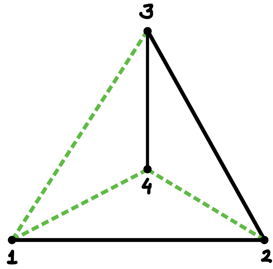
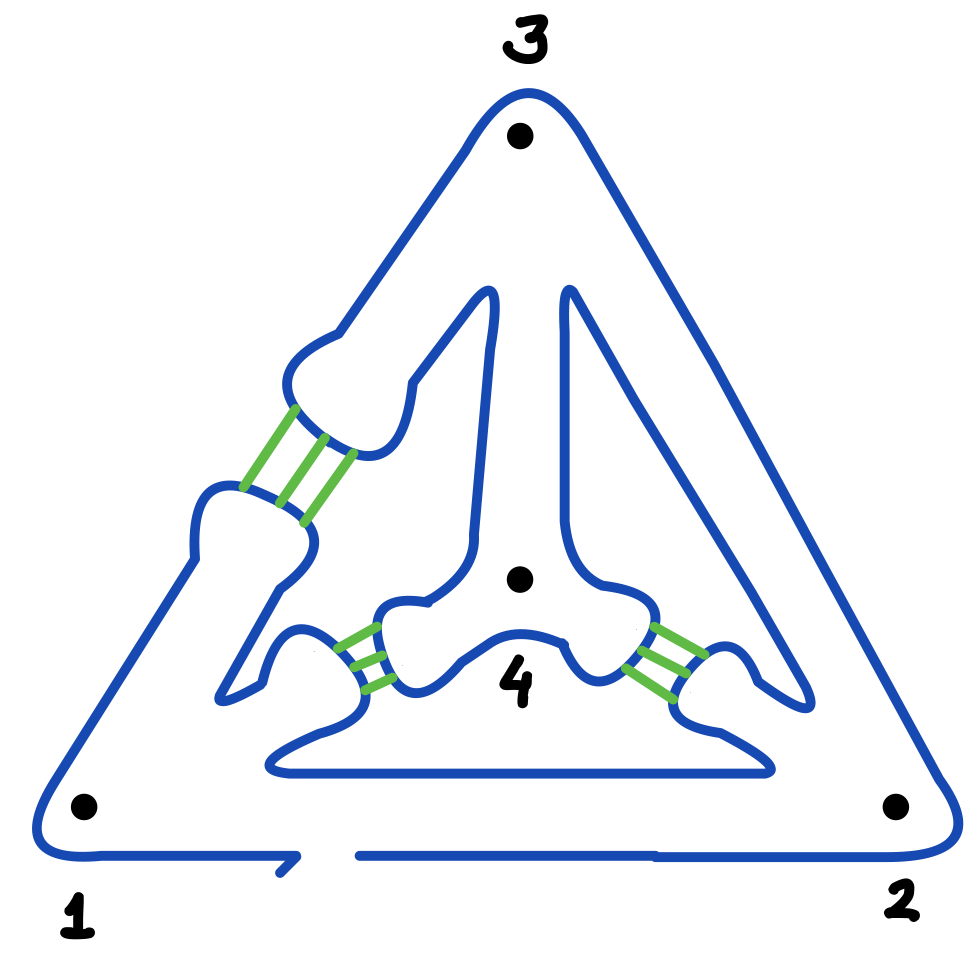

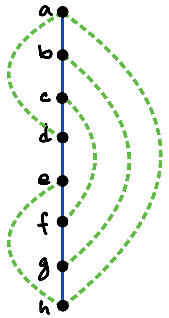
As another example, let us consider the tetrahedron design presented in Figure 4. As shown in Figure 4(a), in this case the spanning tree is a simple 4-vertex path. Figure 4(b) again outlines the corresponding strand route and kissing-loop pair arrangement, with the helix junctions numbered according to their first-visit order. As witnessed by Figure 4(c), this time there is no risk for the polymerase trapping obstacle. That is, every kissing loop closes only after the completion of all the helical pairings that have been initiated after the kissing loop was opened.
Such complete absence of polymerase traps seems like a very particular property, and one may wonder for which kinds of wireframe models this situation can be achieved. As we shall see in the next section, however, such an arrangement of the helical and kissing loop pairings can in fact be found for any connected wireframe graph, by an application of the fundamental algorithmic method of depth-first search [1, Sec. 20.3].
3 Cotranscription-friendly secondary structure design
To streamline the presentation, we assume henceforth that any graph under consideration is connected and undirected, unless stated otherwise. The depth-first search (DFS) method for systematically traversing and labelling a (connected, undirected) graph is presented as Algorithm 1.
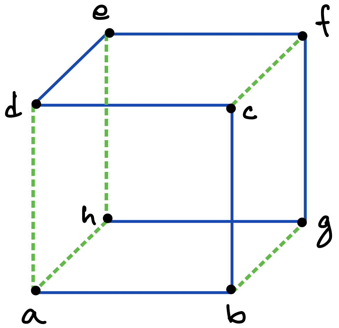
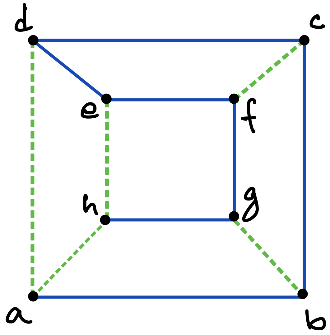

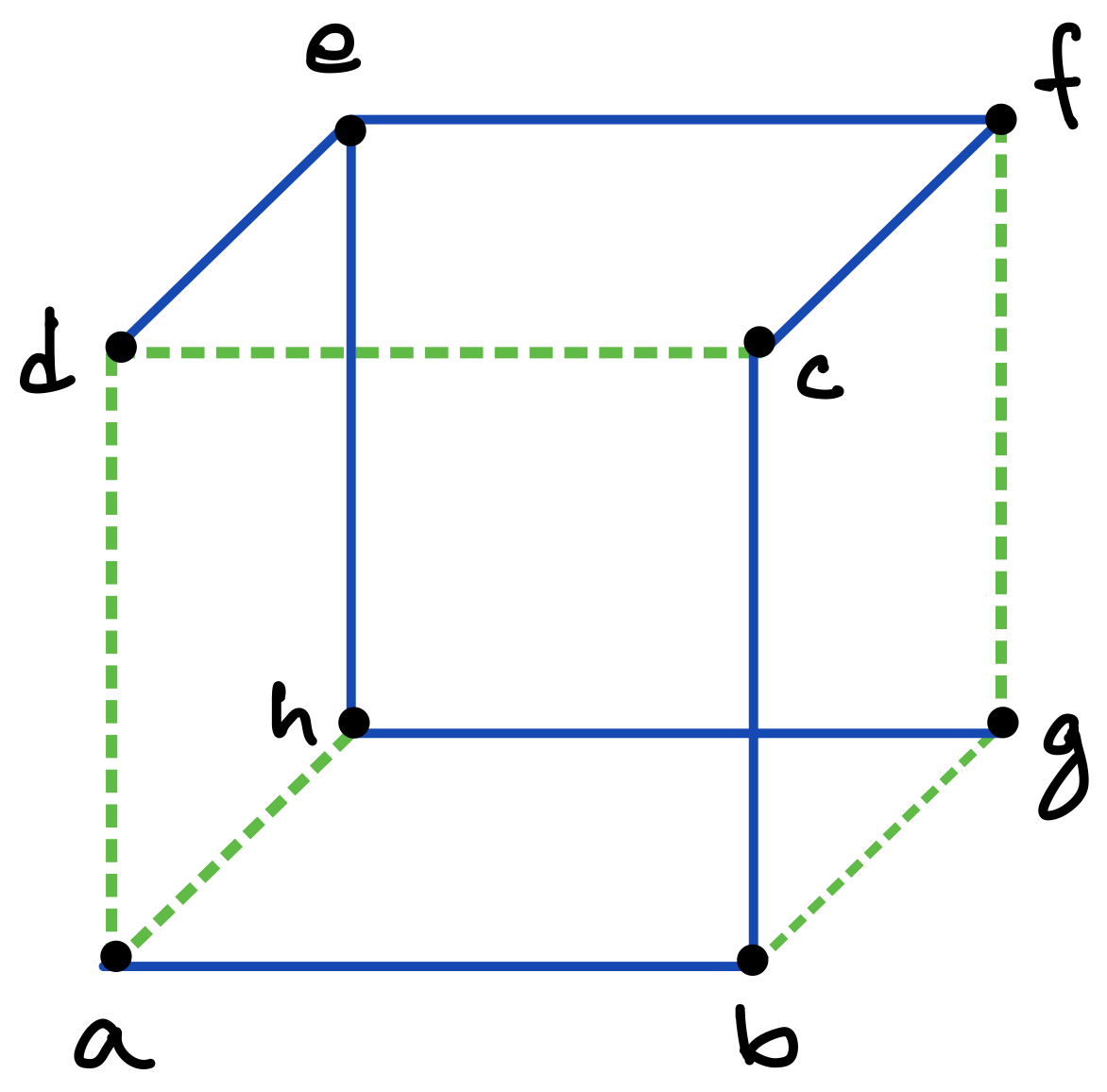
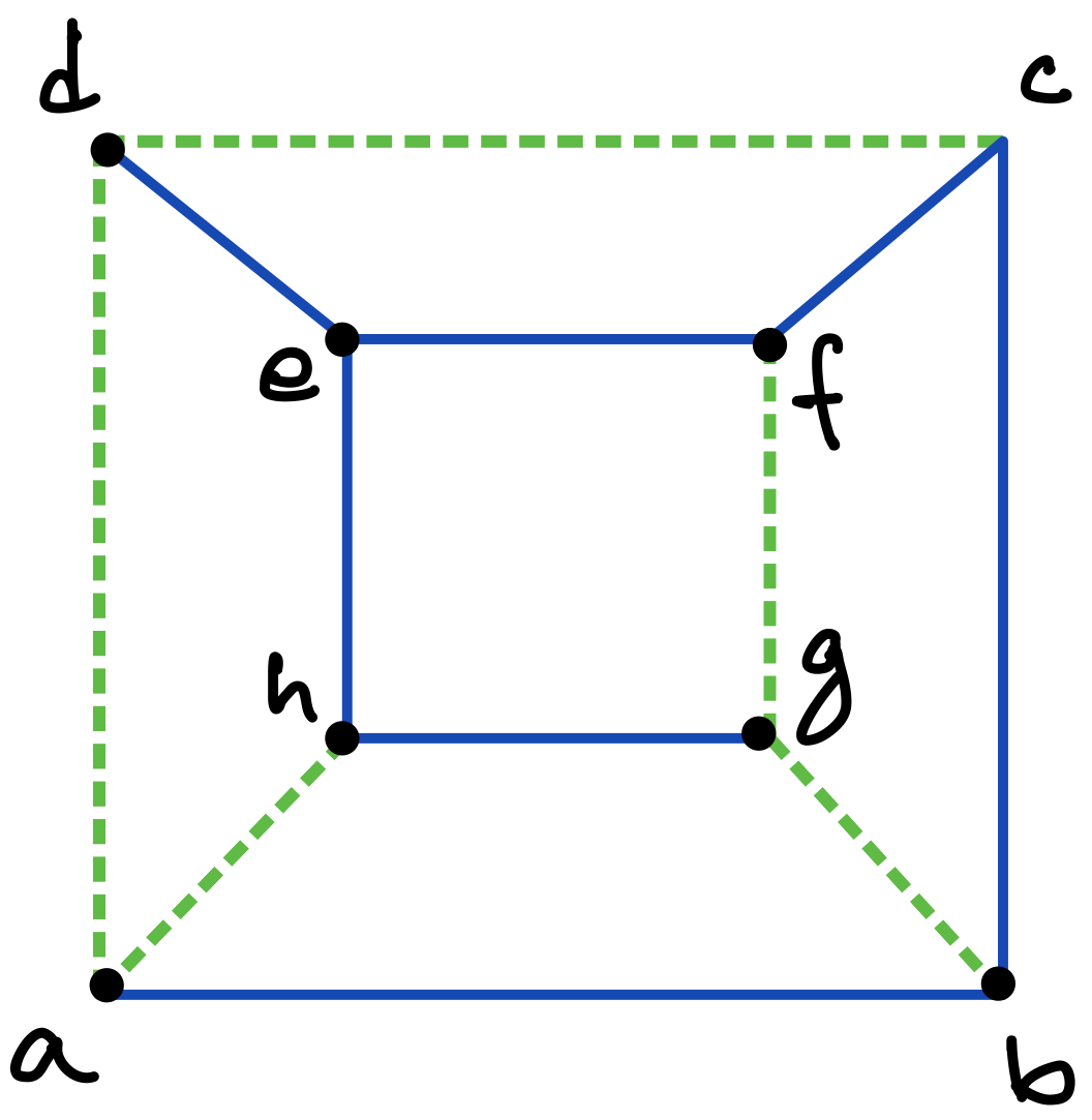
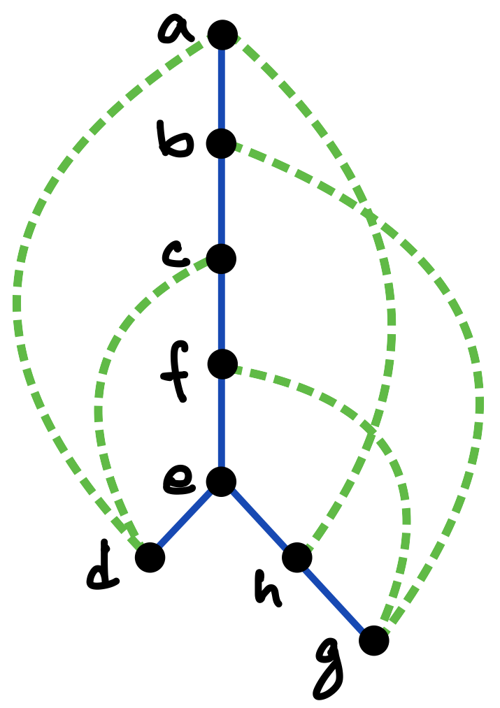

Consider a graph with vertices and edges. Then a DFS traversal of , starting from any chosen root vertex , partitions the set of edges in time in two disjoint classes: tree edges and back edges. The tree edges constitute a spanning tree of , which can be considered to be rooted at and oriented accordingly, whereas the back edges (which constitute the corresponding co-tree ) have the important property that they can always be oriented to point “upward” towards the root of the tree [13]; in other words, there are no “cross edges” connecting two different branches of the directed tree, as exemplified in Figures 5 and 6 (c), and also in Figure 7.333The simple reason for the absence of cross edges is that if for an edge , vertex is still unmarked when the traversal first considers at vertex (or vice versa), then becomes a tree edge.
To make this precise and to introduce another important notion, consider such a DFS (spanning) tree for a graph to be a four-tuple , where is the set of tree edges, is the chosen root which determines the orientation of the tree, and is a pre-ordering that labels the vertices in order of their first visits in the traversal. As discussed above, any edge of is either part of the stem or connects a vertex and its ancestor along the unique path in from the vertex to the root. We often consider as embedded in the plane so that the children of each vertex are ordered from left to right in increasing order of their values. Thus, for example, vertex in Figure 6(c) is presumed to have been visited earlier than vertex in the traversal that created the tree.
A plane embedded DFS tree provides an initial blueprint for designing a cotranscriptionally folding RNA wireframe nanostructure. In the first stage of the design process, the contour of the tree is traced by an RNA strand so that each edge of becomes assembled as an RNA helix, hybridised from two complementary antiparallel domains of . In the second stage the co-tree edges of , which are now back edges of the DFS tree , are constituted as kissing loops made of two half-edge hairpins that extend to meet from the end-vertices of the respective edges.
Let us call the sequence of vertex labels encountered during a walk around the contour of any labelled, plane embedded tree a contour trace or linear arrangement of .444Also known as a “twice-around-the-tree walk” and full walk in [1, p. 1112]. In the special case that is a DFS tree we refer to this sequence as a DFA arrangement based on . By construction, any contour trace of a tree accommodates every edge of exactly twice: firstly, when the traversal crosses in a forward direction, and secondly when the traversal crosses in the opposite direction. Since any DFS tree (or more generally any spanning tree) of a graph with vertices has edges, any DFS arrangement in contains vertex labels. For example, every DFS tree of a tetrahedron is a simple 4-path in its Schlegel diagram, and the corresponding DFS arrangement has the pattern (see Figures 4(a) and (c)).
To complete our blueprint for designing a cotranscriptionally folding RNA nanostructure, the DFS arrangement needs to be augmented into a (domain-level) arc diagram by adding information that indicates when, for each pair of hybridising domains , the forward domain is transcribed and when its complementary reverse domain . For each such pair, these time points are connected by an edge (“arc”), with the first time point considered as the “opening” and the second the “closing” time for this pair. Since in our design scheme, DFS tree edges correspond to helical domains, we correspondingly say that a tree edge is opened when it is crossed by the contour traversal in the forward direction, and closed when it is crossed in the reverse direction. Note that the chosen DFS completely determines the scheduling of the opening and closing pattern of the helical domains.
Let us then consider scheduling the opening and closing times of the back edges, i.e. kissing loops in the eventual RNA nanostructure. Multiple occurrences of internal vertices (neither a root nor a leaf) provide us with freedom to choose, for each back edge , at which visits of and each of the two constituent hairpins of it is to be formed. For each back edge , an occurrence of and that of can be chosen and connected by an arc; then we say that this edge is opened at the time point which corresponds to the left end of the arc, and closed at the right end.
The freedom in timing opening and closing of back edges brings multiple arc diagrams based on the same DFS arrangement. Which should we choose then? Given an arc diagram of , we say that a cycle in is closed at an edge if is in the cycle, and in the arc diagram, all the other edges involved in the cycle have already been closed before is closed. It is known to be kinetically unfavourable to close a cycle at a tree edge. This experimental obstacle motivates our “phloem principle” for ordering back edge connections.555Phloem is a pathway for transporting products of photosynthesis from leaves to the rest of a plant. Recall that the vertices and are labelled with distinct integers and , respectively, and whichever labelled smaller is an ancestor of the other. This principle says that, if , then the assembly of this edge (by a kissing loop) should begin at and end at .
Lemma 1.
The phloem principle prevents any cycle of from being closed at a tree edge.
Proof.
Any cycle of involves a back edge as is acyclic. Let be the set of edges in this cycle; then and are the set of tree edges in the cycle and the set of back edges in the cycle, respectively. The absence of cross edges implies that subtrees of a vertex are connected only via the vertex even in . Hence, the vertex with the smallest -value in a cycle must be incident to a back edge in the cycle; in other words, the following inequality must hold:
Thus, this cycle is closed at the back edge.
This lemma ensures that arc diagrams serve as a blueprint of the polymerase-trap-free co-transcriptional folding pathway as long as they obey the phloem principle. Now we count out any arc diagram that violates the principle. Thus, from now on, an arc diagram of is a pair of a DFS arrangement based on a DFS tree of G and a mapping with such that for all back edge with , if , then , , and . (Arcs for tree edges do not appear anywhere in this definition, but they are uniquely identified by the DFS arrangement.) As , all arc diagrams of are provided with arcs for kissing loops. An arc diagram of the tetrahedron is shown in Figure 4 (d) and those of the cube without any branch and with a branch are shown respectively in Figures 5 (d) and 6 (d), where the arcs for kissing loops are coloured in green, while those for the tree stem are in blue. All of them follow the phloem principle.
The phloem principle does not fully eliminate the freedom in drawing an arc for with since is visited more than once before the last visit at , unless is a leaf. For the sake of the kissing loop crossing (KLX) number, a measure of how good an arc diagram is that we shall discuss next, the arc should be drawn as short as possible, that is, from the last occurrence of to the immediate occurrence of (as is an ancestor of , the search returns to after the last visit to ). However, this criterion of KLX optimisation does not pay any attention to the possible adverse topological effect of focusing a lot of hairpin formations at one time point. Therefore, we have left this freedom in the above definition of arc diagram.
4 Minimising kissing loop crosstalk
A set of kissing loop types should be as orthogonal as possible to minimise the risk of crosstalk, that is the risk of mismatching hairpins hybridising. However, sets of kissing loops that have proven orthogonal enough in the laboratory are limited in size (see, e.g., [10]). The size of largest orthogonal KL sets available in reality serves as a standard for deciding whether a specific (rooted, ordered) DFS tree should be chosen or not. If the design leaves more than this number of kissing loops open simultaneously at any point of folding, it increases the risk of crosstalk.
Recall that any DFS arrangement corresponds one-to-one with a rooted and ordered DFS tree. Given an arc diagram of a DFS tree of a graph , the KLX number of a segment is the number of arcs that cross the vertical line drawn between and . It is defined formally as
| (1) |
The maximum of these values across all segments is the KLX number of this diagram , that is, . Finally, the KLX number of the graph , denoted by , is the minimum among the KLX numbers of all the possible arc diagrams of .
The 1-to-1 correspondence between DFS arrangements and pairs of a graph and its rooted and preordered DFS tree justifies the introduction of the notation as an alias of .
Lemma 2.
Let and be its rooted DFS tree. Let be a (connected) subtree of , and be the subgraph of induced by the vertex set of . Then .
Proof.
It is known that becomes a DFS tree of [13]. Indeed, it suffices to traverse according to the preorder . Note that may preorder the vertices differently and more favorably for the KLX number.
This lemma can be used to prune the search tree for DFS trees with small KLX number, as outlined in Section 6.
As an algorithmic tool, it is useful to exclude some back edges from computing of the KLX number. For a subset of back edges , the KLX number of the segment restricted to , denoted by , can be computed by replacing the occurrence of in Eq. (1) with . It is also convenient to define the KLX number of a tree edge as the number of kissing loops that are opened but yet to be closed during the backward traversal across the edge; the following inequality justifies this definition.
Lemma 3.
In the setting above, let and be the segments that correspond to the forward and backward traversals through an edge of , that is, and . Then .
Proof.
In order for this inequality not to hold, there must be an arc that crosses the segment but not , that is, and . Then would hold, but this contradicts the phloem principle.
Example 4 (KLX number of the cube).
Recall that, with one DFS tree fixed along with the preorder , any back edge with should be opened at the last visit to and then closed ASAP, that is, at the next visit to . No other timing of opening/closing this edge that respects the phloem principle improves in terms of KLX minimisation.
Given a rooted DFS tree without any preorder specified, the sibling order with the minimum KLX number can be computed bottom-up. Consider a branch with its siblings , and suppose that they are visited in this order: first, next, and so on. Then any back edge between the subtree rooted at and a vertex strictly above increments by 1 the KLX number of all the segments corresponding to the edges or all the subtrees below them, although this contribution may not be very clear on the drawing of a DFS tree annotated with back edges, unless the tree is without any branch. Compare (c) with (d) in Figure 6; the back edges and even cross the segments that correspond to the whole traversal of the other subtree of , which consists of the edges and ; this is as clear as day on the arc diagram. The subtrees below are spared this increment because they have been fully explored before such an edge is opened. The back edges that cross over increase the KLX numbers of the path from the root to independently of the order in which the children of are visited. These observations allow the KLX-minimum sibling orders for a given rooted but unordered tree to be computed in a bottom-up manner, starting from leaves, by comparing at each branch (the domainial number of) all permutations of its children.
Let be a vertex with children , be the subtree of below , and be the subtree of below . Let be the set of back edges one of whose endpoints is in , and let be defined analogously with respect to . Suppose that for all edges in with , the KLX numbers restricted to the back edges opened below , that is, , have already been calculated. Let us compute the KLX number restricted less severely to the back edges opened below . The back edges that come from inside and go outside, that is, towards the path of from the root to can be categorised into those ending at and those that go beyond; let us count them and denote the counts, respectively, by and by . Suppose that the children of are visited in this order. The KLX number of an edge in would be then incremented by , that is,
| (2) |
That of an edge would be set as
| (3) |
With the maximum among these numbers in Eqs. (2) and (3), this order competes with the others, and the children of should be ordered according to the one that achieves the minimum; then the KLX number restricted to the back edges opened below should be updated for all tree edges below accordingly.
Ordering the children of even a single vertex in this way may require domainial time in . For the class of 3-regular graphs, quadratic time suffices as a vertex can have at most two children.
5 The minimum kissing loop crossing and minimum tree depth problems
The minimum KLX (kissing loop crossing) number problem (MinKLX) asks, given an undirected, connected graph and a positive integer , if there exists an arc diagram of whose KLX number is at most . This problem is computationally hard as stated in the next theorem; its proof can be found in the technical appendix A.
Theorem 5.
The MinKLX problem is NP-hard.
Another relevant problem is that of determining the depth of the shallowest DFS tree for a given graph , because finding a shallower DFS tree decreases the number of helical domains kept open in parallel, and may result in a sequence with fewer helical domain types. This quantity is closely related to the tree-depth of , which is defined to be the depth of the shallowest DFS tree for a supergraph of . It is NP-hard to compute the tree-depth even for the class of triangulated graphs [2].
Considering the NP-hardness of the MinKLX problem, the only approach to finding a KLX-minimal, cotranscription-friendly designs for a given graph may be via full enumeration of all the DFS trees for . In the next section, we present a branch-and-bound approach to this enumeration process.666As an aside, if one gives up the goal of cotranscription-friendly design, a strand routing that minimises the total number of kissing loops needed to complement it can be found efficiently for any graph, and this number is for many typical wireframe models just zero or one [4].
Before proceeding, let us note that Theorem 5 does not exclude the possibility that KLX-optimal DFS trees could still be found in polynomial time for some graph classes of practical importance such as 3-regular or polyhedral graphs. As any graph can be approximated by a 3-regular one by replacing each vertex by a network of vertices of degree 3, it would be quite interesting to know whether the KLX-minimisation task remains hard for this class. As regards the class of polyhedral graphs, it is known that the MinKLX-related cutwidth minimisation problem (described in the proof of Theorem 5 in Appendix A) is NP-hard for the class of planar graphs with maximum degree 3 [16].
6 Solving the MinKLX and MinTD problems by enumeration
Let us now propose a prototype of algorithmic enumeration of DFS trees for computing the KLX number of a given graph . Algorithm 2 is its pseudocode. Starting from the empty forest, it enumerates the DFS trees by inserting edges of one by one in a predetermined order as a tree edge, that is, as an edge of a DFS tree to be built up. Biconnectedness is utilized, the property of a graph being free from an articulation point, whose removal disconnects the graph. DFS trees of a graph cannot circumvent any biconnected components, or blocks, of . We shall demonstrate how each local branching of a DFS tree orients edges of globally once it is accommodated inside a block of . Orientations thus insisted by more than one such local branching are highly likely to contradict each other, enabling the incremental enumeration of DFS trees to prune the edge-insertion-based search tree. As a shallower tree involves more branches, the tighter an optional upper bound on the depth of DFS trees to be obtained is set, the more effective this block-based pruning should get.
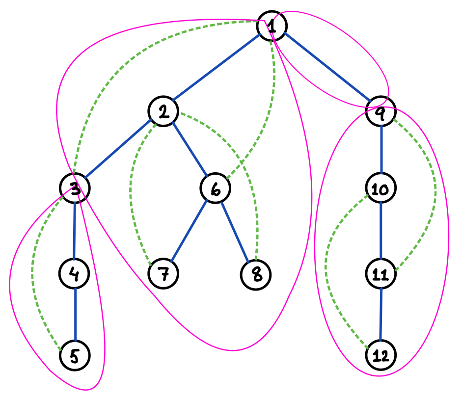
A graph and its spanning tree can be uniquely decomposed into a set of biconnected components, or blocks, , along with a spanning tree that is the intersection of and , the induced subgraph of by ; unless confusion arises, we may call even a block. The blocks can then be uniquely organised into a so-called block-cut tree by connecting two blocks by an edge if these blocks induce the subgraphs of that share (exactly one) vertex in common, which is an articulation point of (see Figure 7 for an example); any articulation point of thus serves as an interface among multiple blocks. We say that is the underlying graph of this block-cut tree. Each block is one of the following types:
-
Branching. if involves a vertex that is incident to at least three edges in (branch);
-
Spinal. otherwise.
Every block contains at least one edge of and no blocks share an edge; hence, the block-cut tree is composed of at most blocks. If a node in a block is incident to at least two tree edges of the block, say , then we say the node is internal. Hence, a spinal block can contain at most two non-internal nodes. Note that an internal node in a spinal block can be a branch of ; unlike a branch in a branching block, this branch is an articulation point of . Therefore, a spinal block can have three or more interfaces. A spinal block consisting of a single edge is particularly called a bridge in [18], and we will borrow this term when it matters whether a spinal block involves an internal vertex or not.
6.1 KLX computation
The decomposition of a graph into blocks may facilitate the computation of the KLX number of , but may not yet save it from brute-forcing sibling orders at every branch, which was discussed at the end of Section 4. Consider a block-cut tree that is free from a branching block; note that the underlying graph may admit a DFS tree with a branch because an internal node of a spinal block can serve as an interface as explained above, and three or more spinal blocks may be incident to an articulation point. The absence of branching block enables the KLX number of the underlying graph according to a DFS tree to be computed as the maximum of those of the blocks according to the respective restrictions of the DFS tree; indeed, it makes no sense for the depth-first-search to stay in a spinal block at any internal interface unless all the other blocks incident to the interface have been already traversed.
The computation of the KLX number of each block according to a DFS tree under construction does not require the DFS tree to be rooted but suffices for each block to know at or beyond which interfaces of them lies the global root. As observed shortly, the DFS tree cannot be rooted at any internal node. Hence, a spinal block can be locally rooted only at one of its two non-internal nodes. Its KLX number does not depend on which of these two vertices the global root is on or beyond. Branching blocks rather restrict where the global root can be due to intrinsic orientation of each of their branches, as we see from now on.
6.2 Pruning
The enumerative computation of the KLX number of can adopt two kinds of pruning strategies.
The one based on the downward closedness of the KLX number along a specific spanning tree (Lemma 2) is simple; while growing a DFS tree as a block-cut forest, once the KLX number of any tree in the forest exceeds a predetermined target value or the current best, then this path of the enumerative search is not worth being pursued further, and hence should be pruned.
The other strategy is based on the following two structural properties of blocks and their DFS rooting from [13]: given a biconnected graph and its spanning tree like the block and its spanning tree ,
-
1.
in order for the spanning tree to be a DFS tree of the graph, it must be rooted at a leaf (of the tree, not of the biconnected graph, all of whose vertices are of degree at least 2);
-
2.
if the spanning tree has a branch, then there exists at most one vertex (indeed, a leaf as just recalled) starting from which the tree can be traversed in a DFS manner.
Let us reproduce a proof for Property 2 (Observation 3.2 in [13]). Suppose there were two such vertices and . If rooted at , the branch, say , has at least two subtrees and , neither of which contains ; without loss of generality, we assume that does not contain . Since the tree becomes a DFS tree by being rooted at , and is not an articulation point, there must be a back edge from to some vertex above along the unique tree path from to the root , but this would become a cross edge once the tree is rather rooted at .
This proof can be applied to observe in our context that every branch inside a branching block is intrinsically oriented, independently of other branches, in such a way that among the edges incident to it, one is incoming while the others are outgoing, as illustrated in Figure 8 (one must be incoming as the branch cannot be a root due to Property 1). Each (local) branch thus globally prohibits a DFS tree of from being rooted at any vertex beyond these outgoing edges. As indicated by red dashed lines in Figure 8, a branch cannot be part of a DFS tree of if it can be bypassed to go back and forth between any two of its three subtrees (second from the left in the figure). A branch inside a block thus orients some edges across the tree that contains the block, and the in-degree of a vertex is defined naturally. Intrinsic orientations imposed by two branches may contradict each other even inside a block, for example, by yielding a vertex of in-degree 2 or higher (second from the right). As soon as the addition of an edge results in such branch(es), a forest under construction is doomed and should be pruned from the search tree.
6.3 Edge insertion and merging of blocks
An edge can be added to grow a forest only if all the following conditions hold: (1) it bridges two separate trees, say and , (connecting two vertices in the same tree would result in a contradictory cycle of tree edges), (2) at least one of the endpoints, say and , is an articulation point of , and (3) or is of in-degree 0; it is then oriented from the endpoint of in-degree 1, if any, to the other (whose in-degree must be 0); if both endpoints are of in-degree 0, then the added edge remains yet-to-be-oriented (see Figure 9). Let us note, related to (2), that a bridge between an internal node and another node is intrinsically oriented away from the internal node in order to prevent a block from being rooted locally at its internal node. Hence, no tree edge can be added between two internal nodes.
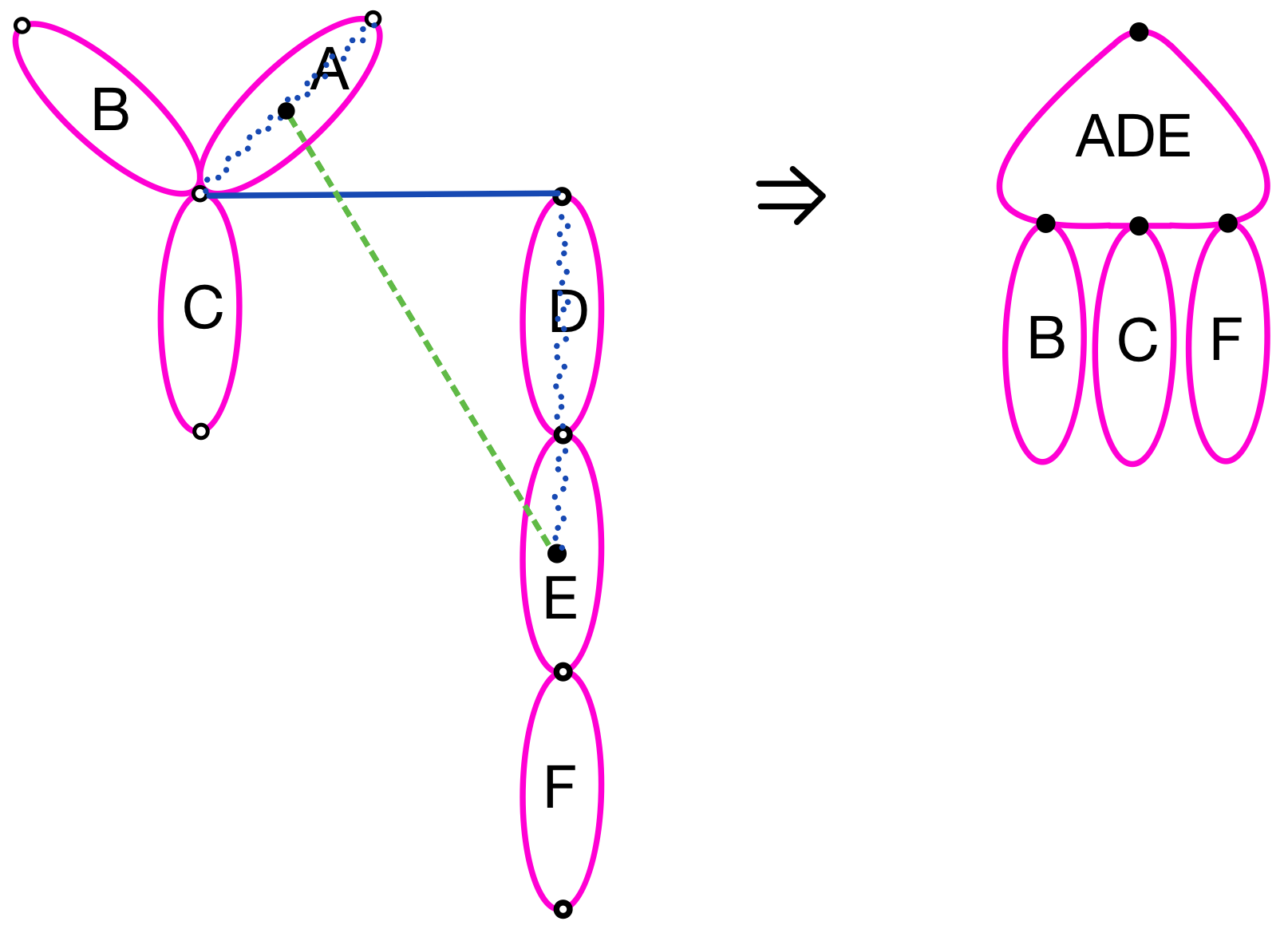
All the other edges between and are ruled out as a candidate of tree edges but introduced rather as an ancillary edge. They are however not guaranteed to be consistent; for example, if one of them is between the leaves and , another is between the leaves and , and all these four vertices are pairwise distinct, then the tree must be rooted globally at or in order for the edge not to become a cross edge, and or claims the ownership of the global root analogously, but these two claims are obviously not compatible. Bridging two trees by an edge may merge some of the blocks in and in into one (see Figure 10). The resulting block can be computed efficiently [18] but its KLX number should also be computable more efficiently from those of the merged blocks and from the cost due to the newly added ancillary edges than being computed from scratch.

7 Examples
The cotranscription-friendly DFS-tree based design method presented in Section 3 is implemented and available for use in the online design tool DNAforge (https://dnaforge.org), together with an option for minimising the KLX cost of the design with a preliminary version of the enumeration method presented in Section 6.777Design method ST-RNA, additional parameters “co-transcriptional route” and “minimise the number of kissing loop sequences”.
| Model | Vertices | Edges | Initial KLX | Min KLX |
|---|---|---|---|---|
| Tetrahedron | 4 | 6 | 3 | 3 |
| Cube | 8 | 12 | 4 | 4 |
| Octahedron | 6 | 12 | 6 | 5 |
| Dodecahedron | 20 | 30 | 9 | 6 |
| Icosahedron | 12 | 30 | 12 | 10 |
| Bunny | 66 | 192 | 60 | 33 |
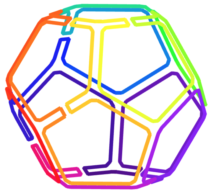
Figures 11 and 12 illustrate some outcomes from the tool. Figure 11 shows designs of wireframe dodecahedra based on a randomly chosen spanning tree (upper row) and a DFS spanning tree (lower row). The DFS-tree based design has also been KLX-optimised, resulting in a reduction from a KLX number of 9 in the initial DFS tree to 6 in the optimal one. (The spanning tree diagrams in Figures 11(b) and (e)) have been manually reconstructed from the tool-generated diagrams in Figures 11(c) and (f).) Figure 12 displays random-tree and DFS-tree designs for a 66-vertex, 192-edge wireframe model of a bunny. Also here the DFS-tree based design has been KLX-optimised, resulting in a KLX number reduction from 60 in the initial DFS tree to 33 in the optimal one. Table 1 summarises the KLX number reductions for some basic mesh models.
8 Conclusions and further work
We have presented models and algorithms for addressing two tasks in secondary structure design for cotranscriptionally folding DNA origami wireframe nanostructures: avoiding the topological folding obstacle of polymerase trapping and minimising the number of distinct kissing loop designs (the KLX number). The key tools in this work have been the algorithmic method of depth-first search in graphs and the ensuing DFS spanning trees. Our branch-and-bound approach to the KLX minimisation problem can also be used for any other effectively computable objective function on DFS trees, such as the DFS tree depth of a given graph (the TD number).
Relevant directions for further work include for instance the following:
-
1.
Nucleotide-level sequence design for DNA origami wireframes in the cotranscriptional setting.
-
2.
Efficient combinatorial algorithms for minimising the KLX and TD numbers in some interesting classes of graphs, such 3-regular or polyhedral graphs, or proving the problems NP-hard in these classes.
-
3.
Efficient fixed-parameter or approximation algorithms for minimising the KLX and TD numbers in some relevant classes of graphs.


References
- [1] Thomas H. Cormen, Charles E. Leiserson, Ronald L. Rivest, and Clifford Stein. Introduction to Algorithms. MIT Press, Cambridge MA, USA, 4th edition, 2022.
- [2] Dariusz Dereniowski and Adam Nadolski. Vertex rankings of chordal graphs and weighted trees. Information Processing Letters, 98(3):96–100, 2006. doi:10.1016/J.IPL.2005.12.006.
- [3] Antti Elonen, Ashwin Karthick Natarajan, Ibuki Kawamata, Lukas Oesinghaus, Abdulmelik Mohammed, Jani Seitsonen, Yuki Suzuki, Friedrich C. Simmel, Anton Kuzyk, and Pekka Orponen. Algorithmic design of 3D wireframe RNA polyhedra. ACS Nano, 16:16608–18816, 2022. doi:10.1021/acsnano.2c06035.
- [4] Antti Elonen and Pekka Orponen. Designing 3D RNA origami nanostructures with a minimum number of kissing loops. In 30th International Conference on DNA Computing and Molecular Programming. Schloss Dagstuhl – Leibniz-Zentrum für Informatik, 2024. doi:10.4230/LIPICS.DNA.30.4.
- [5] Fǎnicǎ Gavril. Some NP-complete problems on graphs. In Proceedings of the 1977 Conference on Information Sciences and Systems, pages 91–95, 1977. URL: https://scispace.com/papers/some-np-complete-problems-on-graphs-4l02n07tlh.
- [6] Cody Geary, Guido Grossi, Ewan K. S. McRae, Paul W. K. Rothemund, and Ebbe S. Andersen. RNA origami design tools enable cotranscriptional folding of kilobase-sized nanoscaffolds. Nature Chemistry, 13(6):549–558, 2021. doi:10.1038/s41557-021-00679-1.
- [7] Cody Geary, Pierre-Étienne Meunier, Nicolas Schabanel, and Shinnosuke Seki. Programming biomolecules that fold greedily during transcription. In 41st International Symposium on Mathematical Foundations of Computer Science, pages 43:1–43:14. Schloss Dagstuhl – Leibniz-Zentrum für Informatik, 2016. doi:10.4230/LIPICS.MFCS.2016.43.
- [8] Cody Geary, Paul W. K. Rothemund, and Ebbe S. Andersen. A single-stranded architecture for cotranscriptional folding of RNA nanostructures. Science, 345(6198):799, 2014. doi:10.1126/science.1253920.
- [9] Cody W. Geary and Ebbe Sloth Andersen. Design principles for single-stranded RNA origami structures. In 20th International Conference on DNA Computing and Molecular Programming, pages 1–19. Springer, 2014. doi:10.1007/978-3-319-11295-4_1.
- [10] Wade W. Grabow, Paul Zakrevsky, Kirill A. Afonin, Arkadiusz Chworos, Bruce A. Shapiro, and Luc Jaeger. Self-assembling RNA nanorings based on RNAI/II inverse kissing complexes. Nano Letters, 11(2):878–887, 2011. doi:10.1021/nl104271s.
- [11] Peixuan Guo. The emerging field of RNA nanotechnology. Nature Nanotechnology, 5(12):833–842, December 2010. doi:10.1038/nnano.2010.231.
- [12] Daniel Jasinski, Farzin Haque, Daniel W. Binzel, and Peixuan Guo. Advancement of the emerging field of RNA nanotechnology. ACS Nano, 11(2):1142–1164, 2017. doi:10.1021/acsnano.6b05737.
- [13] Ephraim Korach and Zvi Ostfeld. DFS tree construction: Algorithms and characterizations. In Graph-Theoretic Concepts in Computer Science, pages 87–106. Springer Berlin Heidelberg, 1989. doi:10.1007/3-540-50728-0_37.
- [14] Di Liu, Cody W. Geary, Gang Chen, Yaming Shao, Mo Li, Chengde Mao, Ebbe S. Andersen, Joseph A. Piccirilli, Paul W. K. Rothemund, and Yossi Weizmann. Branched kissing loops for the construction of diverse RNA homooligomeric nanostructures. Nature Chemistry, 12(3):249–259, 2020. doi:10.1038/s41557-019-0406-7.
- [15] Abdulmelik Mohammed, Pekka Orponen, and Sachith Pai. Algorithmic design of cotranscriptionally folding 2D RNA origami structures. In Unconventional Computation and Natural Computation: 17th International Conference, pages 159–172. Springer, 2018. doi:10.1007/978-3-319-92435-9_12.
- [16] Burkhard Monien and Ivan Hal Sudborough. Min cut is NP-complete for edge weighted trees. Theoretical Computer Science, 58(1):209–229, 1988. doi:10.1016/0304-3975(88)90028-X.
- [17] Erik Poppleton, Niklas Urbanek, Taniya Chakraborty, Alessandra Griffo, Luca Monari, and Kerstin Göpfrich. RNA origami: design, simulation and application. RNA Biology, 20(1):510–524, 2023. doi:10.1080/15476286.2023.2237719.
- [18] Jeffery Westbrook and Robert E. Tarjan. Maintaining bridge-connected and biconnected components on-line. Algorithmica, 7(1):433–464, 1992. doi: 10.1007/BF01758773. doi:10.1007/BF01758773.
Appendix A NP-completeness of the MinKLX problem
Theorem 5.
The MinKLX problem is NP-hard.
Proof.
The proof is based on the proof by Gavril [5] for the NP-hardness of computing the cutwidth of a graph , which asks, given also an integer , to arrange the vertices of along a horisontal line in such a way that, for any vertical line drawn between adjacent vertices, diving into those to its left and those to its right,
The reduction is from Max Cut, which asks to split the vertex set of a given weighted graph into two subsets and so as to maximise the sum of the weights of edges that connect these subsets in . Given a pair of a -vertices graph and a positive integer , let us convert this instance of max cut into an instance of KLX computation problem as follows. With a “large enough” , let be a set of auxiliary “universal” vertices. Let with . Note that, for any , all DFS trees of the complete graph are equivalent, they are indeed a path (no branch), and their KLX number can be computed in polynomial time. Let . Now we are ready to show that has a cut with at least edges between and if and only if the KLX number of is at most .
Firstly, suppose has such a cut, and let and . The linear arrangement of
amounts to a DFS tree of thanks to a universal “glueing” vertex between and (or and ), which are not necessarily connected in (indeed, by definition, they are not connected in iff they are connected in ). With large enough , a tree edge that is crossed by the largest number of back edges is located in the interval , and this number is at most . Thus, the KLX number of is at most .
For the opposite implication, suppose that has a DFS tree whose KLX number is at most . This tree must be “almost” a path in the sense that below a branch, if any, no universal vertex can appear in order not to introduce any cross edge between subtrees below the branch. Therefore, the path from the root of to its first branch, if any, is of length at least , and since is large enough, an edge that determines the KLX number of this DFS tree is somewhere along this path. This path can be extended into a DFS path of the complete graph . The edge which is crossed by back edges is on this path. Among these back edges, at most of them belong to , and the others are edges of the original graph; let be the subset of that consist of these edges. Then, , which implies . Let be the set of vertices in that occur above this edge. Then is a cut which is crossed by at least edges.
