Synchronous Versus Asynchronous Tile-Based Self-Assembly

Becker, Florent; Drake, Phillip; Patitz, Matthew J.; Rogers, Trent A.

doi:10.4230/LIPIcs.DNA.31.9

Synchronous Versus Asynchronous Tile-Based Self-Assembly

Florent Becker

Laboratoire d’Informatique Fondamentale d’Orléans (UR4022), Université d’Orléans, France Phillip Drake

University of Arkansas, Fayetteville, AR, USA Matthew J. Patitz

University of Arkansas, Fayetteville, AR, USA Trent A. Rogers

University of Arkansas, Fayetteville, AR, USA

Abstract

In this paper we study the relationship between mathematical models of tile-based self-assembly which differ in terms of the synchronicity of tile additions. In the standard abstract Tile Assembly Model (aTAM), each step of assembly consists of a single tile being added to an assembly. At any given time, each location on the perimeter of an assembly to which a tile can legally bind is called a frontier location, and for each step of assembly one frontier location is randomly selected and a tile is added. In the Synchronous Tile Assembly Model (syncTAM), at each step of assembly every frontier location simultaneously receives a tile.

Our results show that while directed, non-cooperative syncTAM systems are capable of universal computation (while directed, non-cooperative aTAM systems are known not to be), and they are capable of building shapes that can’t be built within the aTAM, the non-cooperative aTAM is also capable of building shapes that can’t be built within the syncTAM even cooperatively. We show a variety of results that demonstrate the similarities and differences between these two models.

Keywords and phrases:

self-assembly, noncooperative self-assembly, models of computation, tile assembly systems

Funding:

Florent Becker: Research made at a public, state-funded university, thanks to the guarantee of full academic freedom and perennial research funding.

Phillip Drake: This author’s work was supported in part by NSF grant 2329908.

Matthew J. Patitz: This author’s work was supported in part by NSF grant 2329908.

Copyright and License:

2012 ACM Subject Classification:

Theory of computation

\rightarrow

Models of computation

Editors:

Josie Schaeffer and Fei Zhang

Series and Publisher:

Leibniz International Proceedings in Informatics, Schloss Dagstuhl – Leibniz-Zentrum für Informatik

1 Introduction

At the macroscale, humans have mastered the construction of structures with desired spatial and temporal properties. This mastery has provided us with not only entertainment, but also the tools necessary for our survival. As civilization shifts towards a more virtual world and the threats to our survival evolve, a mastery of matter at the macroscale is no longer sufficient. Unfortunately, controlled interaction with the universe at the nanoscale presents significant hurdles. We face major difficulties in observing the universe at the nanoscale, let alone manipulating matter at the this scale. Just as axiomatic models (such as the natural or real numbers) have greatly aided in our understanding (and manipulating) of the universe at the macroscale, axiomatic models of self-assembly have proven successful in allowing us to understand (and manipulate) the universe at the nanoscale. Indeed, such axiomatic models have already enabled the design and implementation of a variety of futuristic nanotechnologies which have a wide range of uses: molecular computers [28], drug delivery [26], and lithographically-patterned electronic/photonic devices [13].

Here, we focus on tile-based, axiomatic models of self-assembly. In these models, the atomic components are square “tiles” which have a “glue” on each of their edges. Growth begins from an initial “seed” assembly and proceeds via single tile attachments. On one end of the spectrum, these single tile attachments occur asynchronously and nondeterministically in a model called the abstract Tile Assembly Model (aTAM). And, on the other end of the spectrum, these single tile attachments occur completely synchronously so that every “frontier” location receives a tile at every step. The fully synchronous model has yet to be studied, so in this paper we introduce a formalization of this model called the synchronous tile assembly model (syncTAM). The syncTAM provides a formal framework for studying the power and limitations of fully-synchronous systems and gives us insight into how we can leverage these synchronization mechanisms to imbue our experimental systems with more power than their asynchronous counterparts.

Perhaps surprisingly, the aTAM gives rise to a variety of complex behaviors. For example, the aTAM is known to be computationally universal [27], intrinsically universal [6], and capable of assembling complex, fractal structures [2]. But, it also has its limitations. For example, the aTAM is limited in the types of interesting, infinite shapes it can assemble [2] and the class of directed, temperature-1 aTAM systems is incapable of computing [19]. Here we investigate whether the syncTAM can overcome some of the limitations of the aTAM and whether a fully-synchronous attachment regime introduces its own set of limitations.

Current ubiquitous technology is capable of physically realizing approximations of asynchronous models of self-assembly, such as the aTAM, but it is unclear if a fully synchronous model can be physically realized in an efficient manner. Inefficient implementations of more synchronous models currently exist. For example, in [25], experimentalists demonstrated the ability to implement a “staged” system where a target structure is assembled in stages by assembling different parts of the structure in separate test tubes and then combining the results to obtain a new substructure which feeds into the next stage. This staging can be thought of as a synchronization mechanism since (if we wait long enough) every assembly will be terminal before it is combined with others. To implement a fully synchronous model using this approach a stage is required for every step making this approach so tedious and laborious it is infeasible.

This work seeks to answer the following question: Is exploring ways to efficiently implement a more synchronous model (than the existing models which are able to be physically realized) a worthy endeavor? We seek to answer this question by comparing the relative powers of an asynchronous model of self-assembly (the aTAM) to a synchronous model of self-assembly (the syncTAM) in terms of shape-building power and computational power.

While the asynchronous mode of tile attachment is the default for self-assembly literature, the synchronous mode of update is the default update model for cellular automata. Fatès, Régnault, Schabanel and others [9, 10, 23, 5] have shown that introducing asynchronism in even the simplest cellular automata vastly alters their behavior. Likewise, Paulevé and Sené [22] show the importance of the choice of update mode in boolean networks. Due to its synchronous nature and the fact that a tile attachment depends on the surrounding neighbors, the class of syncTAM systems can be thought of as a restricted class of freezing cellular automata (CA). Indeed, the class of freezing CA only allows states to increase (according to some ordering), so restricting this class to only allow a single state change and a radius-1 Von Neumann neighborhood yields a class which roughly corresponds to syncTAM systems – it is a slightly more permissive superclass of the syncTAM. Consequently, the results from these models are transitive which provides an interesting mathematical motivation for the study of SyncTAM systems.

Just as comparing asynchronous and synchronous models has been a central theme in cellular automata, our results seek to compare the powers and limitations of the syncTAM with respect to the aTAM. To this end, we begin with formally defining the models used in this paper in Section 2, as well as the formal notions we use to compare the models. Section 3 states the elementary connections between the behavior of the same system in the aTAM versus the syncTAM. In Section 4, we show that there exists shapes that can be assembled in the temperature-1 syncTAM which cannot be assembled at any scale factor in the aTAM (at any temperature). Likewise, that section exposes a set of shapes which can be assembled nondeterministically by an aTAM system but cannot be assembled at any scale factor by a nondeterministic syncTAM system. In Section 5, we show that like the directed aTAM, the directed syncTAM is computationally universal, but unlike the directed, temperature-1 aTAM [19], the syncTAM is computationally universal at temperature 1. To show this, we show that the any temperature-2 compact zig-zag system in the aTAM, can be simulated by a temperature-1 syncTAM system. And, since the class of aTAM temperature-2 compact zig-zag systems is computationally universal [1], the class of temperature-1 syncTAM systems is computationally universal. While previous results about computing at temperature 1 in the aTAM or adjacent models led to very poorly connected assemblies [16, 11, 12, 21, 4], we also show in Section 5.2 that the syncTAM can compute using more well-connected structures.

To make it easier to understand and visualize our results, we have created a web-based simulator for the syncTAM [15] and have implemented all of the systems used in our results [8]. These can all be accessed from http://self-assembly.net/wiki/index.php/Synchronous_Tile_Assembly_Model_(syncTAM).

2 Preliminary Definitions and Models

In this section we define the models and terminology used throughout the paper.

2.1 The abstract Tile-Assembly Model

We work within the abstract Tile-Assembly Model[27] in 2 and 3 dimensions. The abbreviation aTAM refers to the 2D model. These definitions are borrowed from [14] and we note that [24] and [17] are good introductions to the model for unfamiliar readers.

Let $\mathbb{N}$ be the set of nonnegative integers, for $l,u\in\mathbb{Z}$ , let $\llbracket l,u\rrbracket=\{k\in\mathbb{Z}\mid l\leq k<u\}$ . For $n\in\mathbb{N}$ , let $[n]=\llbracket 0,n\rrbracket=\{0,1,...,n-2,n-1\}$ .

Fix $\Sigma$ to be some alphabet with $\Sigma^{*}$ its finite strings. A glue $g\in\Sigma^{*}\times\mathbb{N}$ consists of a finite string label and non-negative integer strength. There is a single glue of strength $0$ , referred to as the null glue. A tile type is a tuple $t\in(\Sigma^{*}\times\mathbb{N})^{4}$ , thought of as a unit square with a glue on each side. A tile set is a finite set of tile types. We always assume a finite set of tile types, but allow an infinite number of copies of each tile type to occupy locations in the $\mathbb{Z}^{2}$ lattice, each called a tile. A glue set $G_{T}$ is the set of all glues associated with a tile set $T$ . Given a direction $d\in\{N,E,S,W\}={\cal D}$ and a tile set $T$ , $G_{T,d}$ is the set of all glues on the edges of tiles in direction $D$ and $g_{t,d}$ is the glue $g$ on tile $t$ in direction $D$ . We write str ${}_{t}(d)$ to denote the strength of $g_{t,d}$ .

Given a tile set $T$ , a configuration is an arrangement (possibly empty) of tiles in the lattice $\mathbb{Z}^{2}$ , i.e. a partial function $\alpha:\mathbb{Z}^{2}\dashrightarrow T$ . Two adjacent tiles in a configuration interact, or are bound or attached, if the glues on their abutting sides are equal (in both label and strength) and have positive strength. Each configuration $\alpha$ induces a binding graph $B_{\alpha}$ whose vertices are those points occupied by tiles, with an edge of weight $s$ between two vertices if the corresponding tiles interact with strength $s$ . An assembly is a configuration whose domain (as a graph) is connected and non-empty. The shape of $X\subset\mathbb{Z}^{2}$ is $\{X+(x,y)|x,y\in\mathbb{Z}\}$ , i.e. the set of all its translations. The shape of an assembly $\alpha$ is the shape $S_{\alpha}$ of its domain: two assemblies have the same shape if they have the same domain modulo translation. An assembly $\alpha$ contains a shape $S$ if there is $s\in S$ such that $s\subset{\rm dom}\;\alpha$ . For some $\tau\in\mathbb{Z}^{+}$ , an assembly $\alpha$ is $\tau$ -stable if every cut of $B_{\alpha}$ has weight at least $\tau$ , i.e. a $\tau$ -stable assembly cannot be split into two pieces without separating bound tiles whose shared glues have cumulative strength $\tau$ . Given two assemblies $\alpha,\beta$ , we say $\alpha$ is a subassembly of $\beta$ (denoted $\alpha\sqsubseteq\beta$ ) if ${\rm dom}\;\alpha\subseteq{\rm dom}\;\beta$ and for all $p\in{\rm dom}\;\alpha$ , $\alpha(p)=\beta(p)$ (i.e., they have tiles of the same types in all locations of ${\rm dom}\;\alpha$ ).

A tile-assembly system (TAS) is a triple $\mathcal{T}=(T,\sigma,\tau)$ , where $T$ is a tile set, $\sigma$ is a finite $\tau$ -stable assembly called the seed assembly, and $\tau\in\mathbb{Z}^{+}$ is called the binding threshold (a.k.a. temperature). If the seed $\sigma$ consists of a single tile, i.e. $|\sigma|=1$ , we say $\mathcal{T}$ is singly-seeded. Given a TAS $\mathcal{T}=(T,\sigma,\tau)$ and two $\tau$ -stable assemblies $\alpha$ and $\beta$ , we say that $\alpha$ $\mathcal{T}$ -produces $\beta$ in one step (written $\alpha\to^{\mathcal{T}}_{1}\beta$ ) if $\alpha\sqsubseteq\beta$ and $|S_{\beta}\setminus S_{\alpha}|=1$ . That is, $\alpha\to^{\mathcal{T}}_{1}\beta$ if $\beta$ differs from $\alpha$ by the addition of a single tile. The $\mathcal{T}$ -frontier is the set $\partial^{\mathcal{T}}\alpha=\bigcup_{\alpha\to^{\mathcal{T}}_{1}\beta}S_{% \beta}\setminus S_{\alpha}$ of locations in which a tile could $\tau$ -stably attach to $\alpha$ . When $\mathcal{T}$ is clear from context we simply refer to these as the frontier locations.

We use $\mathcal{A}^{T}$ to denote the set of all assemblies of tiles in tile set $T$ . Given a TAS $\mathcal{T}=(T,\sigma,\tau)$ , a sequence of $k\in\mathbb{Z}^{+}\cup\{\infty\}$ assemblies $\alpha_{0},\alpha_{1},\ldots$ over $\mathcal{A}^{T}$ is called a $\mathcal{T}$ -assembly sequence if, for all $1\leq i<k$ , $\alpha_{i-1}\to^{\mathcal{T}}_{1}\alpha_{i}$ . The result $\lim\alpha$ of an assembly sequence $\alpha$ is the unique limiting assembly of the sequence. For finite assembly sequences, this is the final assembly; whereas for infinite assembly sequences, this is the assembly consisting of all tiles from any assembly in the sequence. We say that $\alpha$ $\mathcal{T}$ -produces $\beta$ (denoted $\alpha\to^{\mathcal{T}}\beta$ ) if there is a $\mathcal{T}$ -assembly sequence starting with $\alpha$ whose result is $\beta$ . We say $\alpha$ is $\mathcal{T}$ -producible if $\sigma\to^{\mathcal{T}}\alpha$ and write $\mathcal{A}[\mathcal{\mathcal{T}}]$ to denote the set of $\mathcal{T}$ -producible assemblies. We say $\alpha$ is $\mathcal{T}$ -terminal if $\alpha$ is $\tau$ -stable and there exists no assembly that is $\mathcal{T}$ -producible from $\alpha$ . We denote the set of $\mathcal{T}$ -producible and $\mathcal{T}$ -terminal assemblies by $\mathcal{A}_{\Box}[\mathcal{\mathcal{T}}]$ . If $|\mathcal{A}_{\Box}[\mathcal{\mathcal{T}}]|=1$ , i.e., there is exactly one terminal assembly, we say that $\mathcal{T}$ is directed. When $\mathcal{T}$ is clear from context, we may omit $\mathcal{T}$ from notation.

Given TAS $\mathcal{T}$ , we define $\mathcal{S}_{\Box}[\mathcal{T}]=\{S_{\alpha}\mid\alpha\in\mathcal{A}_{\Box}[% \mathcal{T}]\}$ as the set of all shapes of terminal assemblies in $\mathcal{T}$ . Clearly, if $\mathcal{T}$ is directed $|\mathcal{S}_{\Box}[\mathcal{T}]|=1$ . However, even if $\mathcal{T}$ is not directed it may be the case that $|\mathcal{S}_{\Box}[\mathcal{T}]|=1$ (see [3] for an example). In such a case we call the system shape directed.

Given $S$ , a connected set of points in $\mathbb{Z}^{2}$ , we define a version of $S$ scaled by factor $c$ , and denote it by $c\cdot S$ , as $c\cdot S=\{(x,y)\in\mathbb{Z}^{2}\mid(\lfloor\frac{x}{c}\rfloor,\lfloor\frac{y% }{c}\rfloor)\in X\}$ . Intuitively, $c\cdot S$ is a version of $S$ expanded by replacing each point of $S$ by a $c\times c$ square of points. Likewise, for a set $A$ of shapes, $c\cdot A$ is defined as $\{c\cdot S\mid S\in A\}$ .

2.1.1 Zig-zag Tile Assembly Systems

We now provide the definition for a subset of aTAM systems which are known as compact zig-zag systems (originally defined in [4]). These systems have very simple dynamics (the tiles have uniform input and output sides) yet are capable of universal computation – for every Turing machine, there exists a compact zig-zag system which simulates it [4]. Due to their simple dynamics and Turing Universality, these systems are an ideal target for systems with simple mechanisms to simulate to demonstrate they are Turing Universality. This approach has become a paradigm in axiomatic, tile-based self-assembly [4, 16, 11, 12, 21], and we follow this same approach in Section 5.

The following definitions of zig-zag, and compact zig-zag systems are almost identical to those described in [21]. $\mathcal{T}=(T,\sigma,\tau)$ is a zig-zag tile assembly system provided that (1) $\mathcal{T}$ is directed, (2) there is a single $\mathcal{T}$ -assembly sequence $\alpha\in\mathcal{T}$ , with $\mathcal{A}_{\Box}[\mathcal{\mathcal{T}}]=\{\alpha\}$ , and (3) no tile initially binds to an assembly with its north glue. More intuitively, a zig-zag tile assembly system is a system which grows to the left or right, grows up some amount, and then continues growth again to the left or right. Again, as defined in [20], a tile assembly system $\mathcal{T}=(T,\sigma,\tau)$ is a compact zig-zag tile assembly system iff $\mathcal{A}_{\Box}[\mathcal{\alpha}]=\{\alpha\}$ and for every $x\in$ dom $\alpha$ , str ${}_{\alpha(x)}(N)$ + str ${}_{\alpha(x)}(S)<2\tau$ and str ${}_{\alpha(x)}(W)$ + str ${}_{\alpha(x)}(E)<2\tau$ . Informally, this can be thought of as a zig-zag tile assembly system where two $\tau$ -strength tile attachments in a row cannot occur in the same direction. This means a row can never extend by more than one tile over the previous row, and the system is only able to travel upwards one tile at a time before being require to zig-zag again.

2.2 The Synchronous Tile Assembly Model

The Synchronous Tile Assembly Model (syncTAM) is the variant of the aTAM where at every step of assembly, rather that a single location of the frontier being randomly selected to receive a tile, all frontier locations simultaneously receive a tile each. As the frontier of a system can grow arbitrarily large, the number of tiles added per assembly step may also grow arbitrarily large. As in the aTAM, if any single frontier location allows for $\tau$ -strength binding of tiles of multiple types, one of those types is non-deterministically chosen for each such location.

We formally define the syncTAM in the same way as the aTAM with the exception of the definition of a single step in the assembly sequence. Give a syncTAS $\mathcal{S}=(T,\sigma,\tau)$ and two $\tau$ -stable assemblies $\alpha$ and $\beta$ , we say that $\alpha$ $\mathcal{S}$ -produces $\beta$ in one step, written $\alpha\to^{\mathcal{S}}_{1}\beta$ , if $\alpha\sqsubseteq\beta$ and ${\rm dom}\;(\beta)\setminus{\rm dom}\;(\alpha)=\partial^{\mathcal{S}}(\alpha)$ . Note that like in the aTAM, we define $\partial^{\mathcal{S}}(\alpha)$ to be the set of locations where a tile can $\tau$ -stably attach to $\alpha$ . The syncTAM inherits all other definitions and notation from the aTAM.

To distinguish between a tile assembly system (a.k.a. TAS) in the aTAM versus one in the syncTAM, we will use the term syncTAS to refer to a TAS in the syncTAM.

3 Similarities between the aTAM and the syncTAM

In this section we show that directed and shape-directed aTAM systems behave equivalently in the syncTAM. That is, given a tile set $T$ , seed $\sigma$ , and temperature $\tau$ , if $(T,\sigma,\tau)$ is used as an aTAM system and that system is directed (resp. shape directed), then when $(T,\sigma,\tau)$ is used as a syncTAM system the same unique terminal assembly (resp. assembly shape) is produced. Although these are relatively straightforward results, they demonstrate the types of systems, namely those with reduced nondeterminism, which are invariant to the differing dynamics of the models.

Lemma 1.

Let $\mathcal{S}=(T,\sigma,\tau)$ be a syncTAM system and $\mathcal{T}=(T,\sigma,\tau)$ be an aTAM system composed of the same components. If $\alpha$ and $\alpha^{\prime}$ are assemblies of $\mathcal{S}$ such that $\alpha\rightarrow_{\mathcal{S}}^{1}\alpha^{\prime}$ , then $\alpha\rightarrow_{\mathcal{T}}\alpha^{\prime}$ .

Proof.

Let $\mathcal{S}=(T,\sigma,\tau)$ be a syncTAM system and $\mathcal{T}=(T,\sigma,\tau)$ be an aTAM system composed of the same components. Furthermore, assume that $\alpha$ and $\alpha^{\prime}$ are assemblies of $\mathcal{S}$ such that $\alpha\rightarrow_{\mathcal{S}}^{1}\alpha^{\prime}$ .

Let $F$ be the set of pairs consisting of a frontier location of $\alpha$ and a tile that can $\tau$ -stably attach to $\alpha$ at that location such that for every pair $(p,t)\in F$ , $\alpha^{\prime}(p)=t$ . Intuitively, $F$ is the set of all tiles (a tile type and position) such that adding the tiles of $F$ to $\alpha$ yields $\alpha^{\prime}$ . Our construction of $F$ ensures that all the positions contained in the pairs are distinct (that is, no two pairs contain the same position), and every tile can attach $\tau$ stably to $\alpha$ . Consequently, we can construct a valid $\mathcal{T}$ -assembly sequence from $\alpha$ to $\alpha^{\prime}$ through single tile attachments from the tiles in $F$ . Indeed, let $(f_{i})_{i=1}^{n}$ be an enumeration of the set $F$ . Define $\alpha_{0}=\alpha$ and $\alpha_{i}=\alpha_{i-1}\cup f_{i}$ . Then $\alpha_{0}\to\alpha_{1}\to\dots\to\alpha_{n}$ is a valid assembly sequence since all tiles can $\tau$ -stably attach and none prevent the others from binding, and $\alpha_{n}=\alpha^{\prime}$ . $\hfill\blacktriangleleft$

Section 3 shows that each single step of syncTAM assembly can be matched by a set of steps of an equivalent aTAM system. Thus, beginning from the same seed assembly, successive applications of that lemma show that any assembly that is producible in a syncTAM system is also producible in the equivalent aTAM system.

Lemma 2.

Let $\mathcal{T}=(T,\sigma,\tau)$ be an arbitrary directed (resp. shape directed) aTAM system. Then the syncTAM system $\mathcal{S}=(T,\sigma,\tau)$ , composed of the same components, is also directed (resp. shape directed) and terminally produces exactly the same singular terminal assembly (resp. singular shape for all terminal assemblies) as $\mathcal{T}$ .

Proof.

Let $\mathcal{T}=(T,\sigma,\tau)$ be an arbitrary directed aTAM system, and let $\mathcal{S}=(T,\sigma,\tau)$ be composed of the same components. By definition, $\mathcal{T}$ has exactly one terminal assembly which we denote by $\alpha$ . We claim that this is also the only terminal assembly of $\mathcal{S}$ . Suppose, for the sake of contradiction, this was not the case. That is, suppose $\alpha^{\prime}\in\mathcal{A}_{\Box}[\mathcal{\mathcal{S}}]$ and $\alpha^{\prime}\neq\alpha$ . Let $\alpha_{i}$ be a $\mathcal{T}$ -assembly sequence such that $\alpha_{0}=\sigma$ and $\lim\alpha_{i}=\alpha$ and let $\alpha^{\prime}_{i}$ be a $\mathcal{S}$ -assembly sequence such that $\alpha^{\prime}_{0}=\sigma$ and $\lim\alpha^{\prime}_{i}=\alpha^{\prime}$ . Then it follows from Lemma 3 that $\alpha^{\prime}_{i}$ is a valid $\mathcal{T}$ assembly sequence which contradicts our assumption $\mathcal{T}$ is directed.

The argument for the shape directed version of the lemma is similar, but instead of assuming (for the sake of contradiction) that $\alpha^{\prime}\neq\alpha$ as above, we assume for the sake of contradiction that $S_{\alpha}\neq S_{\alpha^{\prime}}$ . The rest of the argument remains the same. $\hfill\blacktriangleleft$

Thus, the two lemmas presented here show that systems with limited nondeterminism produce the same assemblies (and/or shapes) in both the aTAM and the syncTAM. This completely changes in the general case: the additional power, and constraints, imposed by the global synchronization of the syncTAM also provide for separations between the models, which we now present in Sections 4 and 5. This culminates in Theorem 8 which demonstrates a shape $S$ such that no aTAM system can assemble $S$ , but there exists a syncTAM system which assembles $S$ .

4 Separating the aTAM and the syncTAM by Shape Production

The difference between the aTAM and the syncTAM is manifest in the shapes an sets of shape each model is able to assemble. This section exhibits a set of shapes and a shape which are exclusive to one of the models, respectively the aTAM and the syncTAM. Much like how we ignore constants when studying the runtime of algorithms, often in tile-based self-assembly the size of a “pixel” in the shape is discounted. In our results, it will not just be the shape which is unobtainable in the “wrong” model, but all of its scaled versions. Likewise, while in each case, the “right” model can assemble those shapes without collaboration (i.e. at temperature $1$ ), no amount of collaboration can help the wrong model in obtaining them.

4.1 Sets of Shapes that need the Asynchronism of the aTAM

The synchronism of the syncTAM can act as a constraint, making it impossible for a single syncTAS to match the dynamics of the more asynchronous aTAM. Namely, we exhibit a simple aTAM system that can create an infinite set of different shapes, while any syncTAS must be constrained to only forming a subset of them.

Impossibility proofs for the aTAM often rely on the Window Movie Lemma [20] (an overview of which can be found in Section A.2). Alas, it does not hold in the syncTAM, as the delay between successive attachments along the window can be used by either side to avoid being “fooled” by the change in the other. On the other hand, in the syncTAM, positions cannot remain attachable for an arbitrarily long time, which prevents the delaying tactics the aTAM can use. Hence, the fooling lemmas for the syncTAM differ from those of the aTAM. The following two lemmas capture this and will prove sufficient for the purpose of this paper.

The first limit of syncTAM systems is that they cannot leave positions attachable for an infinitely long time (and this holds for any infinite assembly sequence, which differs from the aTAM).

Lemma 3 (Completion).

Let $\mathcal{S}$ be a syncTAM system. For any infinite assembly sequence $\alpha$ of $\mathcal{S}$ , $\lim\alpha$ is a terminal production: $\lim\alpha\in\mathcal{A}_{\Box}[\mathcal{\mathcal{S}}]$ .

Proof.

Assume $z$ is a frontier location in $\lim\alpha$ . There is a subset $N$ of the neighbors of $z$ such that a tile could attach $\tau$ -stably to the tiles of $\lim\alpha$ within $N$ . Let $t$ be the last time a tile was attached in $N$ . Then $z$ belongs to the frontier of $\alpha_{t}$ , has been filled at time $t+1$ and cannot be empty in $\lim\alpha$ .

Thus, the frontier of $\lim\alpha$ is empty and $\lim\alpha$ is a terminal production. $\hfill\blacktriangleleft$

The second limitation of syncTAM systems is that if their productions can avoid some patterns for an arbitrarily long time, then they have a terminal production avoiding those patterns.

Lemma 4 (Compacity).

Let $F$ be a set of finite shapes of $\mathbb{Z}^{2}$ . Let $\mathcal{S}$ be a syncTAM system with, for each $k\in\mathbb{N}$ , a production $P_{k}\in\mathcal{A}[\mathcal{\mathcal{S}}]$ producible in $k$ assembly steps that does not contain $F$ .

Then there is a terminal production $T\in\mathcal{A}_{\Box}[\mathcal{\mathcal{S}}]$ such that $\operatorname{dom}(T)$ does not contain any element of $F$ .

Proof.

The attachment sequence $(\beta_{i})_{i\geq 0}$ of $\mathcal{S}$ (defined recursively as follows) is such that from each $\beta_{i}$ , infinitely many $P_{i}$ can be $\mathcal{S}$ -produced:

$\blacksquare$

$\beta_{0}$ is the seed assembly, from which all the $P_{i}$ can be produced,
$\blacksquare$

for each $i$ , since $\beta_{i}$ is a finite production, it has only finitely many descendants (productions $d$ such that $\beta_{i}\to^{\mathcal{S}}_{1}d$ ). Since $\beta_{i}$ $\mathcal{S}$ -produces infinitely productions $P_{j}$ , one of its descendants must also produce infinitely many $P_{j}$ ; pick that descendant to be $\beta_{i+1}$ .

By Section 4.1, $T=\lim\beta$ is a terminal production, yet it cannot contain any element of $F$ . If it did contain an $X\in F$ , since $X$ is finite, there would be a finite $f$ such that $\beta_{f}$ contains $X$ and that $\beta_{f}$ would not be compatible with any of the $P_{k}$ . $\hfill\blacktriangleleft$

Theorem 5.

There is an aTAM system $\mathcal{A}$ such that for any syncTAM system $\mathcal{S}$ and scale factor $c\geq 1$ , $\mathcal{S}_{\Box}[\mathcal{\mathcal{S}}]\neq c\cdot\mathcal{S}_{\Box}[% \mathcal{\mathcal{A}}]$ .

Proof.

Let $\mathcal{A}$ be the aTAM system of Figure 1. As depicted in Figure 1, let $A(d,r,u)$ for $d\geq 0,r\geq 0,u\geq-4$ be the subset of $\mathbb{Z}^{2}$ defined by:

A(d,r,u)=(\llbracket 0,r\rrbracket\times{0})\cup({0}\times\llbracket-d,0% \rrbracket)\cup(\llbracket 0,\min(u+4,4)\rrbracket\times\{-d\})\cup(\{3\}% \times\llbracket-d,u-d\rrbracket)

Figure 1: Left, the tile types of the temperature

1

aTAM System

{\cal A}

. There is a line between two tile edges whenever their glue match, edges without incident lines have a

0

-strength glue. The seed is the red

s

tile. Each of the tiles

r, d, u

can grow arbitrarily long tile segments, respectively to the right, upwards and downwards. To the right, a typical production

A(u,d,r)

of

{\cal A}

, then the three sets of terminal assemblies of

{\cal A}

:

A_{\Gamma}

,

A_{d}(d)

and

A_{\sigma}(d)

. The yellow parts at the top of the productions are the copies of

\Gamma

, the gray parts at the bottom, the copies of

U_{4}

, and the encircled part at the top is the copy of

B_{5}

.

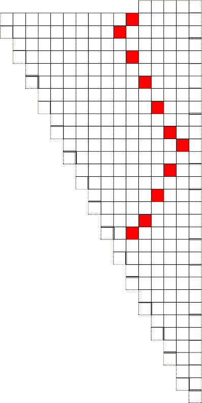
The shape of any assembly of ${\cal A}$ is of the form $A(d,r,u)$ for some values of $d, r$ and $u$ . The quantity $u$ starts from negative values so as to correspond to the number of $u$ tiles of the assembly, as shown on Figure 1. The “ $-3$ rd, $-2$ nd, $-1$ st and $0$ th $u$ tiles” are the $4$ tiles at the bottom of the assembly between the $d$ and $u$ arms. The values of $d, r$ and $u$ are not independent:

$\blacksquare$

when $d=0$ , $u=-4$ : the bottom part can only grow after the lower arm has grown
$\blacksquare$

only one of $u>d$ and $r>3$ can hold at once, because of the competition between the two arms for position $(3,0)$ .

The shapes of the terminal productions of ${\cal A}$ are of one of the following forms:

$\displaystyle A_{\Gamma}$	$\displaystyle=$	$\displaystyle A(+\infty,+\infty,-3)$
$\displaystyle A_{d}(d)$	$\displaystyle=$	$\displaystyle A(d,3,+\infty)$
$\displaystyle A_{\sigma}(d)$	$\displaystyle=$	$\displaystyle A(d,+\infty,d)$

$\blacktriangleright$ Remark 6.

Having glanced at Figure 1, it may seem straightforward that ${\cal A}$ cannot be simulated by a syncTAS $\mathcal{S}$ , assuming $\mathcal{S}$ proceeds like A, with two concurrent arms starting from the top-left: the horizontal arm cannot wait for a downwards arm which may never be coming back to the meeting point; yet, it can never turn to the north without knowing that the other arm will come back. The remainder of the proof essentially makes that argument robust against $\mathcal{S}$ placing its seed elsewhere, using its scale factor to synchronize the two arms, or any other shenanigans. $\lrcorner$

Back to the proof, consider the following shapes:

$\blacksquare$

$\Gamma=\{(0,0),(0,-1),(1,0)\}$ ,
$\blacksquare$

$U_{4}=\{(0,1),(3,1)\}\cup(\{0\}\times\llbracket 0,3\rrbracket)$ , a 4-tile wide U,
$\blacksquare$

$B_{5}=(\llbracket 0,4\rrbracket\times\{0\})$ , a $5$ -tile horizontal bar.

Any terminal production of ${\cal A}$ must contain $\Gamma$ , and either $B_{5}$ or a translated copy of $U_{4}$ .

Assume now there is a syncTAM system $\mathcal{S}$ and an integer $c$ such that $\mathcal{S}_{\Box}[\mathcal{\mathcal{S}}]=c\cdot\mathcal{S}_{\Box}[\mathcal{% \mathcal{A}}]$ . Then for any terminal production $T_{\mathcal{S}}$ of $\mathcal{S}$ , there is a terminal production $T_{\cal A}$ of ${\cal A}$ and a vector $\vec{\tau}$ such that ${\rm dom}\;T_{\mathcal{S}}=c\cdot{\rm dom}\;T_{\cal A}+\vec{\tau}$ . Note that while $c$ is the same for all productions, $\vec{\tau}$ may be different for each of them.

All terminal productions of $\mathcal{S}$ must have a translated copy of $c\cdot\Gamma$ , and a translated copy of either $c\cdot U_{4}$ or $c\cdot B_{5}$ . By compacity (Section 4.1), there is an integer $t(\{c\cdot\Gamma\})$ such that any production at time $t\geq t(\{c\cdot\Gamma\})$ has $(c\cdot\Gamma)+\vec{\tau}$ as a subset of its shape for some vector $\vec{\tau}\in\mathbb{Z}^{2}$ . Likewise, there is an integer $t(\{c\cdot U_{4},c\cdot B_{5}\})$ such that any production at time $t\geq t(\{U_{4},B_{5}\})$ has either $(c\cdot U_{4})+\vec{\tau}$ or $(c\cdot B_{5})+\vec{\tau}$ as a subset of its shape for some vector $\vec{\tau}\in\mathbb{Z}^{2}$ .

Let $T=\max(t(\{c\cdot\Gamma\}),t(\{c\cdot U_{4},c\cdot B_{5}\}))$ , the shape of any production $P$ of $\mathcal{S}$ at time $T$ contains: a copy of $c\cdot\Gamma$ , and a copy of either $c\cdot U_{4}$ or $c\cdot B_{5}$ . Because $P$ was produced in time $T$ , the distance between its copy of $c\cdot\Gamma$ and its copy of $c\cdot B_{5}$ or $c\cdot U_{4}$ is less than $2T+1$ .

Let $d=\left\lceil\frac{2T+1}{c}\right\rceil+1$ . The terminal production $A_{d}(d)$ of ${\cal A}$ contains neither a copy of $B_{5}$ , nor a copy of $U_{4}$ within distance $\frac{2T+1}{c}$ of its copy of $\Gamma$ : its unique $\Gamma$ is at $(0,0)$ , while the leftmost tile of its $U_{4}$ is at $(0,-d)$ . Hence, there is no production of $\mathcal{S}$ at time larger than $T$ whose shape is contained in $c\cdot A_{d}(d)$ . Therefore, there is no final (infinite) production of $\mathcal{S}$ with shape $c\cdot A_{d}(d)$ , which is a contradiction. $\hfill\blacktriangleleft$

4.2 A Shape Demanding the Synchronization of the syncTAM to Self-assemble

This section exhibits a simple (infinite) shape which cannot be uniquely self-assembled in the asynchronous aTAM, while it can be assembled at temperature $1$ by a relatively simple syncTAS. Essentially, the synchronous nature of the syncTAM allows for a (shape) directed syncTAS that creates a single shape using an infinite series of rows of tiles growing from opposite directions that are always guaranteed to meet near a central location, while the asynchronous aTAM cannot guarantee that both sides will always grow at the same speed and therefore the meeting locations may differ and the aTAM system must also be able to produce other, non-target shapes.

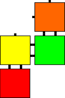
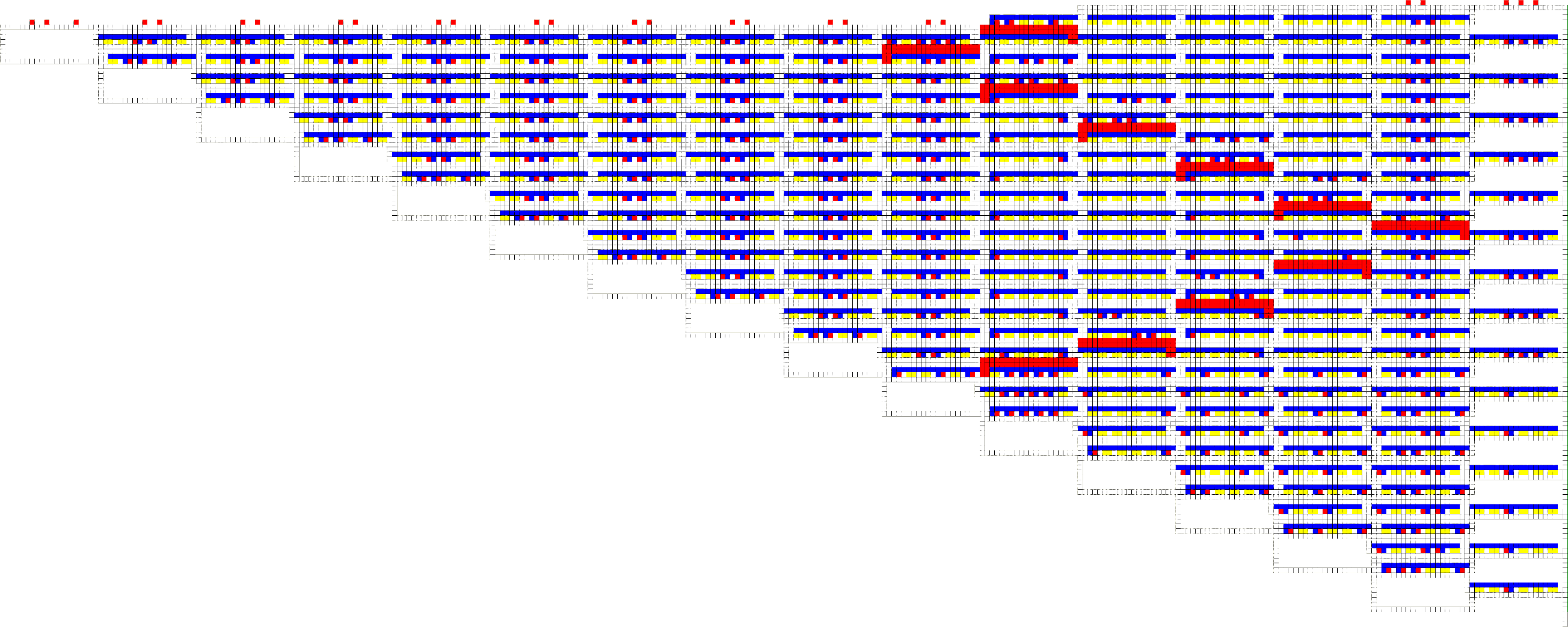
Consider the syncTAM system $\mathcal{S}$ of Figure 2(a), and let $V$ be the following subset of $\mathbb{Z}^{2}$ , as depicted on that figure:

V=\{(0,0)\}\cup L\cup R\cup\bigcup_{k>0}\left(B^{-}_{k}\cup T^{-}_{k}\cup B^{+% }_{k}\cup T^{+}_{k}\right)

where:

the left branch: is the set $L=\{(-x,x),(-x-1,x)|x\in\mathbb{N}\}$ ,
the right branch: is the set $R=\{(x,x),(x+1,x)|x\in\mathbb{N}\}$ ,
the left bar at height $k$: is the set $B_{k}^{-}=\{(x,4k)|x\in\llbracket-4k+1,1\rrbracket\}$ , and
the right bar at height $k$: is the set $B^{+}_{k}=\{(x,4k+1)|x\in\llbracket 0,4k\rrbracket\}$
the left thumbs: form the set $T^{-}_{k}=\{(2x+1,4k+1)|x\in\llbracket-2k,0\rrbracket\}$
the right thumbs: form the set $T^{+}_{k}=\{(2x,4k)|x\in\llbracket 0,2k\rrbracket\}$

(a) The tiles of the temperature

1

syncTAM system

\mathcal{S}

(the seed is the yellow

s

tile), and a portion of the infinite shape

V

assembled by

\mathcal{S}

. Growth begins from the seed tile at the bottom and proceeds with the diagonal “arms” growing upward to the left and right, and with red rows growing right from the left arm, and blue rows growing left from the right arm, at every 4th step. The green part is

L

, the orange and brown part is

R

, the blue parts are the

B^{+}_{k}\cup T^{+}_{k}

, while the red parts are the

B^{-}_{k}\cup T^{-}_{k}

.

(b) Using pumping in the aTAM on the two windows depicted at the top to produce an illegal production at the bottom: the right part has grown past the middle.

Figure 2: A syncTAM system assembling a shape that cannot be obtained in the aTAM.

$\blacktriangleright$ Remark 7.

The system $\mathcal{S}$ is directed and $V$ is the shape of its unique terminal assembly. $\lrcorner$

Theorem 8.

There is no TAS system which uniquely assembles $V$ at any scale factor: for all TAS systems ${\cal A}$ and $c\geq 1$ , $\mathcal{S}_{\Box}[\mathcal{{\cal A}}]\neq c\cdot\mathcal{S}_{\Box}[\mathcal{% \mathcal{S}}]$ .

Proof.

Consider an integer $c$ and a TAS system ${\cal A}$ with $g$ different glues. Given a producible assembly $A$ in ${\cal A}$ and a position $z\in\mathbb{Z}^{2}$ , we say that $A$ has entered $p$ if $c\cdot\{z\}\cap{\rm dom}\;A\neq\varnothing$ .

As in [18], define a glue movie on a set of edges $W$ of the grid to be the order of placement, position and glue type for each glue that appears along the window $W$ in an assembly sequence. There are at most $p=2(4c)!(4c)^{g}$ possible glue movies of ${\cal A}$ on a window of size $4c$ . Indeed, there are $(4c)^{g}$ potential scenarios for the tuple of glue types that lie along one side of the window, and there are $(4c)!$ permutations of this tuple, and we get the $2$ in the beginning of the expression from the fact that we must consider both sides of the windows. Assume without loss of generality that $p>4$ and thus $p$ is even.

Consider an assembly sequence $(\alpha)_{i=0}^{\infty}$ of ${\cal A}$ reaching a terminal production; the shape of $\lim\alpha$ is $c\cdot V$ translated by a vector $\vec{\tau}\in\mathbb{Z}^{2}$ . From now on, all coordinates are translated by $-\vec{\tau}$ , so that ${\rm dom}\;(\lim\alpha)=c\cdot V$ .

Let $t^{-}$ be the minimal $t$ such that there are $p+3$ different positions of $B_{4p+2}^{-}$ where $\alpha_{t}$ has entered. Likewise, $t^{+}$ is the time where $p+3$ different positions of $B_{4p+2}^{+}$ have been entered by $\alpha_{t^{+}}$ . Assume for now that $t^{+}<t^{-}$ , and let $A=\alpha_{t^{+}}$ .

Pose $A_{0}=A$ , and $x^{\max}_{0}=c(4p+2)-2$ . Let $W_{x}$ be a rectangle of height $4c$ , width $p+1$ with its lower-left corner at $(x,(16p+7)c$ . In $A_{0}$ , on any window $W_{x}$ with $x\in\llbracket x^{\max}_{0}-p-1,x^{\max}_{0}\rrbracket$ there are no tiles touching the left, upper and lower edges of $W_{x}$ , while there must be at least a tile inside $W_{x}$ . Thus, there are only $p$ different window movies possible for all windows $W_{x}$ , while there are $p+1$ such windows. There must be $a, b$ such that the Window Movie Lemma of [18] applies between $W_{a}$ and $W_{b}$ . This begets a production $A_{1}$ in which at most $p+3$ positions have been entered in $B_{4p+2}^{-}$ , while $p+4$ positions have been entered in $B_{4p+2}^{+}$ . This process can be iterated by posing $x^{\max}_{i}=x^{\max}_{0}-i$ , until $i=3cp$ . In $A_{3cp}$ , the right bar from the right extends past the midpoint, and the resulting shape is not a subset of $V$ . We have obtained a terminal shape that is not included in $V$ and a contradiction.

If $t^{-}<t^{+}$ , the reasoning is the same, with $x$ varying at iteration $i$ between $x^{\min}_{i}$ and $x^{\min}_{i}+p+1$ , with $x^{\min}_{i}=-x^{\max}_{i}$ . Then $A_{3p}$ extends straight past the midpoint. $\hfill\blacktriangleleft$

5 Separating the aTAM and the syncTAM by $\tau=1$ Computation

In this section we show that directed, temperature-1 syncTAM systems are computationally universal (while this is not the case for directed, temperature-1 aTAM systems [19]). To prove this, we show that any temperature-2, compact zig-zag aTAM system can be simulated by a temperature-1 syncTAM system. The result then follows from a previous result: For every Turing machine $M$ , there exists a temperature-2 compact zig-zag aTAM system which simulates it [4]. This approach (often used to show a class of temperature-1 systems are computationally universal [16, 11, 12, 21, 4]) benefits from the fact that rigorous definitions are already in place defining simulation between the necessary models. We end the section by showcasing a class of computationally universal temperature-1 syncTAM systems wherein each row is connected to the next by two north-south attachments, a level of connectivity not seen in previous simulations of TMs by non-cooperative tile assembly systems.

5.1 Computation at Temperature 1 in the syncTAM

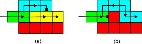
We first give a high-level overview of how a temperature-2, compact zig-zag aTAM system $\mathcal{T}$ simulates a Turing machine $M$ . At a high level, $\mathcal{T}$ simulates $M$ by exposing glues on the north of assembly which encode the symbols on the tape of $M$ . One time step of a TM is simulated by growing a row which “zigs” (a row which grows to the right) and then a row which “zags” (a row which grows to the left). If the head transitions to the right during the step, this occurs during the growth of the “zig” row. A left transition, is performed during the growth of the “zag” row. In either case, the cooperative placement of tiles (that is, the requirement that a tile binds with two strength-1 glues) allows for information about the head of the state to be propagated through the east and west glues while information about the symbols stored in the tape is propagated through the south and north glues. See part (a) of Figure 5 for an example which highlights the movement of the head as an aTAM system simulates a Turing machine. For a more in depth explanation of how compact zig-zag systems simulate Turing machines, see [4].

The generally used technique (employed in [16, 11, 12, 21, 4]) is to get one of the two necessary inputs of a simulated cooperative binding via a glue attachment, and the other via carefully regulated growth around some sort of hindrance provided by geometry or glue repulsion. The subsets of tiles that perform the simulation of a single cooperative binding are referred to as bit-readers and bit-writers, i.e. tiles that grow a portion of an assembly capable of logically reading or writing bit values.

Theorem 9.

Let $\mathcal{T}=(T,\sigma,2)$ be an arbitrary compact zig-zag aTAM system. There exists a syncTAS system $\mathcal{S}=(S,\sigma^{\prime},1)$ such that $\mathcal{S}$ simulates $\mathcal{T}$ at scale factor $O(\log|G_{T,N}|)$

Refer to caption — Figure 3: An example of writing and reading a bit in the syncTAM. The red tiles represent the bit-writers. (a) A value of $0$ was first written by the red tiles. Later, growth from the west causes placement of the green tiles. The rightmost green tile initiates the growth of the yellow and blue paths. Since the yellow path is shorter it always arrives at the second yellow location first, blocking placement of a blue tile later. The yellow path proceeds, encoding that a value of $0$ was read. (b) A value of $1$ is encoded in the geometry of the red tiles. The northernmost red tile blocks the growth of the yellow path allowing the blue path to complete instead, encoding that a value of $1$ was read.

The system $\mathcal{S}$ simulates $\mathcal{T}$ by assembling $n\times m$ blocks of tiles, which we call macrotiles. These macrotiles map to tiles in $T$ under some macrotile representation function, $R$ . We design $\mathcal{S}$ so that it behaves exactly like $\mathcal{T}$ under the macrotile representation function.

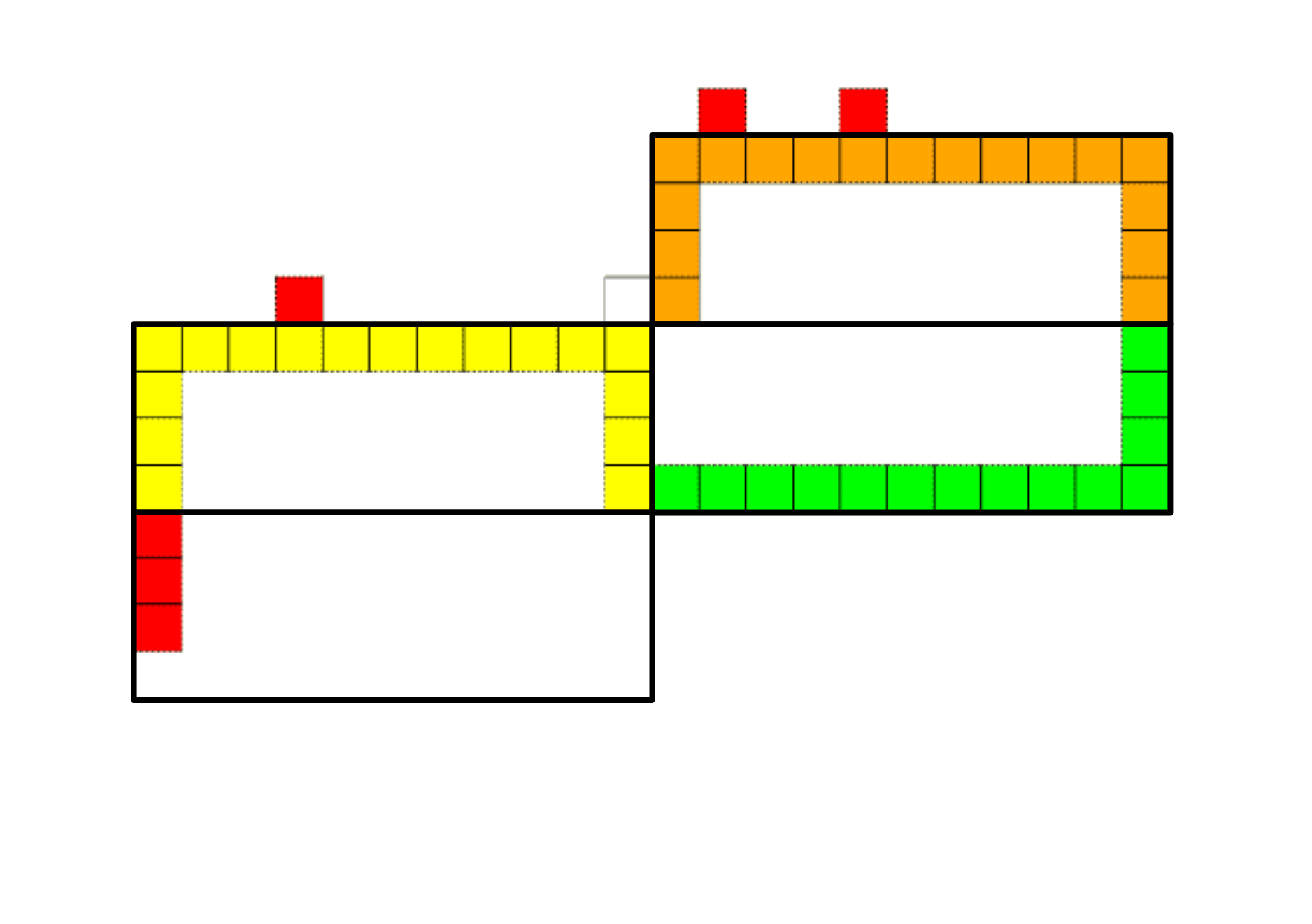
It is straightforward to design $\mathcal{S}$ to simulate the strength- $2$ attachments in $\mathcal{T}$ , but simulating cooperative binding attachments (attachments where a tile binds with two strength-1 glues) in $\mathcal{T}$ using $\mathcal{S}$ is much less obvious. Suppose that we want to simulate the attachment of a tile which binds cooperatively via its west and south glues. At a high-level, our construction uses gadgets to encode the northern strength-1 glues on a preceding row as geometry. Information about the strength-1 east glues being simulated by the macrotile to the west is presented as a glue on the macrotile boundary. From this glue, gadgets assemble which “read” the existing geometry below. Details about how these gadgets read and write the geometry is shown in Figure 3. The end result of this is the exposure of a glue which is unique to the simulated glue from below and the simulated glue from the preceding tile in the row. Consequently, this glue allows a tile to attach that causes the macrotile to map to the correct tile $t$ under the representation function, and it allows for a chain of bit-writers which encode information about the north glue of $t$ to grow into the neighboring macrotile region to the north. After the bit-writers are assembled, a path of tiles grow to expose a glue corresponding to the west glue of $t$ on the boundary of the next macrotile region.

We now provide a sketch of the proof.

Proof.

Let $\mathcal{T}=(T,\sigma,2)$ be a compact zig-zag TAS. We now describe how to construct a syncTAS $\mathcal{S}=(S,\sigma_{s},1)$ which simulates $\mathcal{T}$ (under the definition of simulation formally defined in Section A.1). Note that under the definition of simulation, the domain of a macrotile is square. Our construction is designed to work with a notion of simulation that allows for rectangular macrotile domains, but we could design our tile set to pad the lengths of the paths that it grows to account for square macrotile domains.

We construct $\mathcal{S}$ so that the macrotiles over $\mathcal{S}$ consist of translations of subassemblies, also referred to as gadgets, called bit-writers, bit-readers and translators. We define 0-bit-writers and 1-bit-writers to be any translation of the red subassemblies shown in Figure 3. We refer to these collectively as just bit-writers. A bit-writer encodes (in binary) the label of a strength 1, north glue of a tile in $\mathcal{T}$ so that it can be “read” by a bit-reader contained in the macrotile region above it which will enable $\mathcal{S}$ to determine which tile the macrotile should map to in $\mathcal{T}$ . Gadgets called 0-bit-readers and 1-bit-readers “read” this information (accomplished through growing exactly one of two paths depending on the geometry). We define these to be translations of the non-red subassemblies shown in Figure 3. Note that each of these gadgets grow from the same tile, but the existing geometry of the bit-writers (which were guaranteed to have previously completed growth) give rise to exactly one of the two subassemblies growing. A translator gadget is a translation of a subassembly that maps to a tile, denote this tile $t^{\prime}$ , which binds with a strength $2$ glue. This subassembly is simply a path of tiles that grows from the “beginning” of a macrotile to the “beginning” of the next macrotile. The exact beginning and end position of this path depends on the location of the strength $2$ glue on $t^{\prime}$ and the locations of its output glue. In the case that the tile to which a translator gadget belongs contains a strength-1 glue to its north, the translator may contain a chain of bit-writers in order to express this glue.

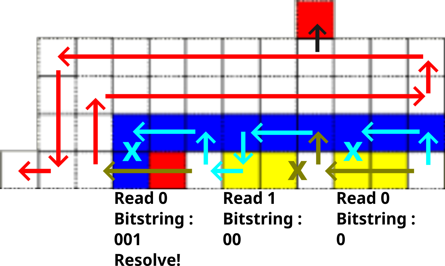
We now describe the idea behind bit-writers and bit-readers. At a high level, bit-readers attempt to grow two paths of tiles, say a $0$ -path and a $1$ -path. The bit-writers are designed to block exactly one of these paths, leaving the “surviving” path to constitute a read of its relevant bit. To accomplish this behavior, we design the $1$ -path to be exactly one tile longer than the $0$ -path, so if a previously assembled $0$ -bit-writer does not block the $0$ -path, then it will be one tile “ahead” of the $1$ -path, and thus block the $1$ -path, hence, a 0 is read. However, if the $1$ -bit-writer blocks the $0$ -path, then the $1$ -path will not be blocked, and a 1 a is read. Figure 3 shows the details of this mechanism. The glues in these surviving paths then “know” the bit that was encoded in the geometry by the bit-writer. It can use this knowledge for subsequent tasks such as assembling its own bit-writers.

We now describe the desired behavior of $\mathcal{S}$ , and then we describe how we can construct the tile set $S$ to obtain this desired behavior. We describe the behavior of $\mathcal{S}$ in two scenarios. The first scenario we consider is the scenario where $\mathcal{S}$ needs to assemble a macrotile that maps to a tile (under the macrotile representation function) that attaches cooperatively. The second scenario we consider is the scenario where $\mathcal{S}$ is growing a macrotile that “simulates” the attachment of a tile in $\mathcal{T}$ via a strength-2 attachment.

In the following discussion, let $\vec{t}=((x^{\prime},y^{\prime}),t)$ , for $t\in T$ , be a tile (i.e. a placed instance of a tile type) in a producible assembly of $\mathcal{T}$ , and let $REG(x,y)$ be the macrotile region which maps to the tile at location (x,y) (in $\mathcal{T}$ ) under the macrotile representation function. That is $REG(x,y)$ is the set $\{(i,j)|(mx\leq i\leq m(x+1))\textrm{ and }my\leq j\leq m(y+1)\}$ . Then, intuitively, $REG(x\textquoteright,y\textquoteright)$ is the region which maps to $\vec{t}$ , $REG(x\textquoteright-1,y\textquoteright)$ is the region which maps to the tile to the west of $\vec{t}$ , call this tile $\vec{t}_{w}$ , and $REG(x\textquoteright,y\textquoteright-1)$ is the region which maps to the tile to the south of $\vec{t}$ , call this tile $\vec{t}_{s}$ .

In the first case, assume $\vec{t}$ is a tile in a producible assembly of $\mathcal{T}$ which binds into the assembly cooperatively using two strength- $1$ glues. Without loss of generality, we assume the two “input” glues $\vec{t}$ uses to bind to the assembly are on its west and south. The case where they are on its east and south is symmetric. We now describe how $\mathcal{S}$ leverages bit-writers and bit-readers to assemble a macrotile in the macrotile region $R$ that maps to $\vec{t}$ under the macrotile representation function. Before a bit-reader begins assembling in a macrotile region, our construction of $\mathcal{S}$ ensures a chain of bit-writers has assembled in the southern region of the macrotile. The bit-writers are chained together such that the last tile in a bit-writer exposes a glue on its east so that another bit-writer can begin growing from this glue. This chain of bit-writers is assembled during the growth of the macrotile to the south, and it encodes the label of the north glue of $\vec{t}_{s}$ in binary. For each strength 1 glue on the west of a tile in $T$ , say $g_{w}$ , there is a unique chain of bit-readers that grows from a glue that corresponds to $g_{w}$ . So, a chain of bit-readers specific to the east glue of $\vec{t}_{w}$ starts assembling from the southwest most corner of $REG(x\textquoteright,y\textquoteright)$ . Each bit-reader in this chain is unique to the binary sequence read up to that point, so that by the time the bit-reading chain is assembled, there is a tile placed at the end of the bit-reading chain that is specific to the east glue of $\vec{t}_{w}$ and the north glue of $\vec{t}_{s}$ . It is at this point that the macrotile representation function begins mapping the subassembly contained in $REG(x\textquoteright,y\textquoteright)$ to $\vec{t}$ . A new path of tiles begins assembling from this glue which grows bit-writers in the macrotile region to its north, that is the region $R(x\textquoteright,y\textquoteright+1)$ , encoding the north output glue of $\vec{t}$ . Then a path grows from the end of this chain of bit-writers to place a glue on the border of the macrotile region directly to the west of $R$ , that is the region $R(x\textquoteright+1,y\textquoteright)$ , which is specific to the east output glue of $\vec{t}$ . The process then repeats.

Note that $\log|G_{T,N}|$ bits are necessary to express the label of a strength-1 north glue in $\mathcal{T}$ . As such, each macrotile that simulates a tile that has a strength-1 glue on its south must include $\log|G_{T,N}|$ bit-readers, and each macrotile that expresses a strength-1 north glue must grow $\log|G_{T,N}|$ bit writers. Therefore, with a bit-reader/writer length of $4$ , our macrotiles are of scale $4\times O(\log|G_{T,N}|)$ .

The second case we consider is where $\vec{t}$ is a tile in a producible assembly of $\mathcal{T}$ that binds into the assembly via a strength- $2$ glue. In this case, the simulator simply grows a path of tiles (which are unique to that glue and, hence, uniquely determine the tile in $T$ the macrotile needs to map to under the representation function) to place a glue at the beginning of the next macrotile region so that the growth process can repeat. This path may include a chain of bit-writers, in the case that the tile exhibits a strength-1 glue to its north. The exact path that is grown depends on the exact locations of the input and output glues on $\vec{t}$ .

Compact zig-zag systems are singly-seeded (consequently their seed tile exposes a strength-2 glue if growth proceeds) by definition, so to form the seed for our simulator, we simply place a tile so that it exposes a glue that begins the simulation process described above.

We now describe the tiles in $S$ that lead to the desired behavior described above. For each east/west glue in $T$ , we add tiles to $S$ with unique glues that assemble a chain of bit-readers. Note that the glues for each bit-reader in the chain are distinct and we add tiles for each position in the chain which assemble a 0-bit-reader and a 1-bit-reader. In addition, for each tile in $T$ , we add unique tiles to $S$ that grow the bit-writer corresponding to the label of the strength-1 north glue (if it exists) and grows a path to the macrotile boundary exposing a glue corresponding to the east/west glue. An example macrotile, including both a chain of bit-readers and bit-writers is displayed in Figure 4(c). Finally, for each translator we add tiles to $S$ that assemble the path of tiles composing the translator and have unique glues that do not interact with any other gadgets in $\mathcal{S}$ . The tiles required to construct the translators of an example compact zig-zag system are displayed in Figure 4(b).

The above construction correctly simulates $\mathcal{T}$ provided that a bit-reader never attempts to grow into a macrotile region without a bit-writer chain. Note that provided a strength-1 glue is not exposed at the end of a row in $\mathcal{T}$ , we have constructed $\mathcal{S}$ to essentially consist of one long path of tiles so that the bit-writer chain must be assembled before a bit-reading gadget reaches the macrotile region. To ensure no strength-1 glue is exposed at the end of a row in $\mathcal{T}$ , we modify $\mathcal{T}$ so that the north glues of the tiles at the end of each row are marked with a special symbol. We leverage this special glue to further modify $\mathcal{T}$ so that no strength-1 glue is ever exposed at the end of the row. Consequently, no bit-reader will ever attempt to “read” an empty macrotile region and the construction is correct.

An example compact zig-zag aTAM system, along with a syncTAM system that simulates it is displayed in Figure 5. Along with this, a script which may be used to convert an arbitrary compact zig-zag TAS to a syncTAS may be found at [8]. $\hfill\blacktriangleleft$

Corollary 10.

For every standard Turing machine $M$ and input $w$ , there exists a temperature-1 syncTAM system that simulates $M$ on $w$ .

This follows directly from Lemma 7 of [4] (i.e. that, given an arbitrary Turing machine $M$ and input $w$ , there exists a compact zig-zag that simulates $M$ on $w$ ), and Theorem 9.

5.2 Greater Assembly Connectedness at Temperature 1

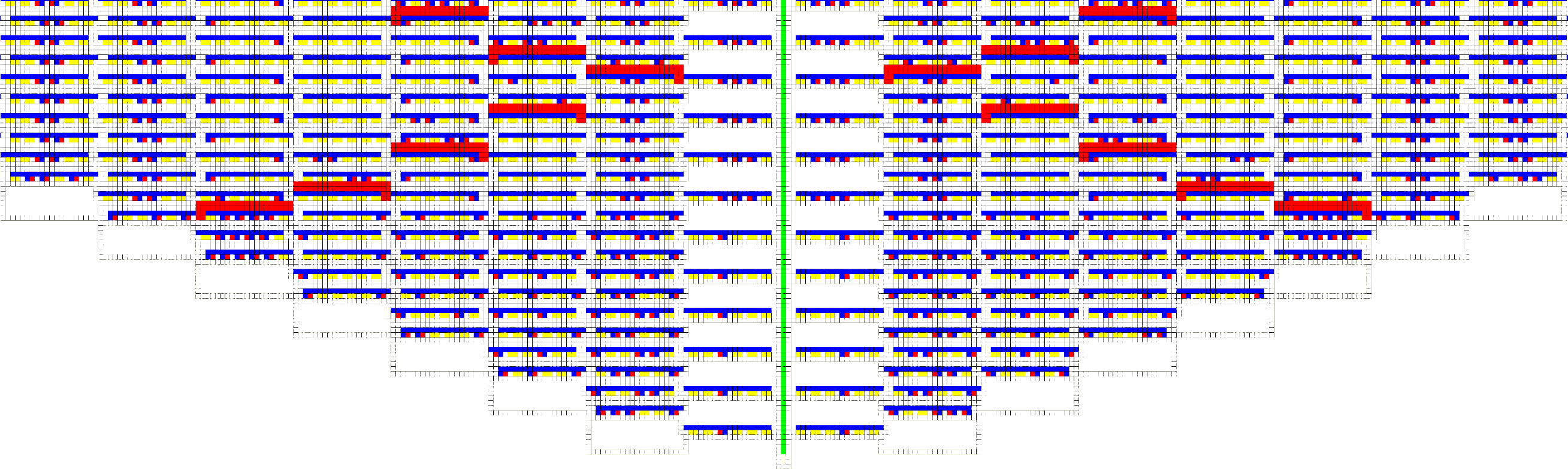
As previously mentioned, a variety of tile-based, temperature-1 models of self-assembly are computationally universal. Discrimination between types of tiles representing the correct input values from two different locations can be easily done using multiple glue bonds in a temperature-2 system. However, in a temperature-1 system this discrimination must be performed using some sort of hindrance that prevents incorrect tile types from binding while still always allowing the correct tile type to bind. This hindrance (often provided by geometry, as with the “blocker” tile in our construction for Section 5.1) allows for algorithmically correct growth but necessarily results in assemblies with extremely sparse connectivity. The resulting have a binding graph that is a single-tile-wide path that zig-zags and folds back over itself, row by row, throughout the entire assembly. Each row, of increasingly great length, is attached by a single glue bond to the row below it. This results in an assembly that would be extremely “floppy” if physically realized. In all others models where such temperature-1 computation is achieved, this floppiness appears unavoidable since any exposed glue that may be intended to bind to a later-growing portion of the assembly and provide greater stability could, at any time, initiate its own growth (which may or may not agree with correct later growth). However, the precise synchronization enabled by the syncTAM can ensure that two separately-growing portions of an assembly of the same size can be guaranteed to complete at the exact same time, and we can leverage this to provide greater connectivity.

In order to provide this greater connectivity, we must ensure that each row which is placed in the zig-zag TM grows in from both directions, this means that the binding graph will have two paths for each zig / zag of the system, which converge, and diverge in repeating intervals. To accomplish this, the compact zig-zag TM construction displayed in Figure 5 may be reflected along the y axis, and connected to the east, and west of a single-tile seed such that the two identical simulations assemble in parallel.

Due to the synchronous nature of the syncTAM, both identical simulations will arrive at a single-tile wide unoccupied column during the exact same step. All macrotiles which contain a side abutting this unoccupied column only belong to the tiles which grow on the far-east edge of the original aTAM system, and thus only appear abutting the unoccupied column. As such, those tiles may have the side abutting the unoccupied column modified such that they contain a unique “connecting” glue, to which a single “connector” tile type may connect, “stitching” both sides of the assembly together.

As a result of the connector tile stitching both sub-assemblies together along each row, each row will therefore be connected to the row previous by at least two north-south attachments, one on the original TM simulation, and one on its reflection. Consequentially, every row is connected to the previous row by two or more glues. A snapshot of this connected assembly is shown in Figure 6. As with the section previous, a script which takes as input a TM definition, and outputs a more connected syncTAS which simulates it may be found at [8].

References

[1] Gagan Aggarwal, Michael H. Goldwasser, Ming-Yang Kao, and Robert T. Schweller. Complexities for generalized models of self-assembly. In Proceedings of ACM-SIAM Symposium on Discrete Algorithms, 2004.
[2] Florent Becker, Daniel Hader, and Matthew J. Patitz. Strict Self-Assembly of Discrete Self-Similar Fractals in the abstract Tile Assembly Model, pages 2387–2466. SIAM, 2025. doi:10.1137/1.9781611978322.80.
[3] Nathaniel Bryans, Ehsan Chiniforooshan, David Doty, Lila Kari, and Shinnosuke Seki. The power of nondeterminism in self-assembly. Theory of Computing, 9:1–29, 2013. doi:10.4086/toc.2013.v009a001.
[4] Matthew Cook, Yunhui Fu, and Robert T. Schweller. Temperature 1 self-assembly: Deterministic assembly in 3D and probabilistic assembly in 2D. In SODA 2011: Proceedings of the 22nd Annual ACM-SIAM Symposium on Discrete Algorithms. SIAM, 2011. doi:10.1137/1.9781611973082.45.
[5] Isabel Donoso Leiva, Eric Goles, Martín Ríos-Wilson, and Sylvain Sené. Asymptotic (a)synchronism sensitivity and complexity of elementary cellular automata. In Proceedings of LATIN’24, volume 14579 of LNCS, pages 272–286. Springer, March 2024. doi:10.1007/978-3-031-55601-2_18.
[6] David Doty, Jack H. Lutz, Matthew J. Patitz, Robert T. Schweller, Scott M. Summers, and Damien Woods. The tile assembly model is intrinsically universal. In Proceedings of the 53rd Annual IEEE Symposium on Foundations of Computer Science, FOCS 2012, pages 302–310, 2012. doi:10.1109/FOCS.2012.76.
[7] Phillip Drake, Daniel Hader, and Matthew J Patitz. Simulation of the abstract tile assembly model using crisscross slats. In 30th International Conference on DNA Computing and Molecular Programming (DNA 30)(2024), pages 3–1. Schloss Dagstuhl – Leibniz-Zentrum für Informatik, 2024.
[8] Phillip Drake and Matthew J. Patitz. Synchronous TAM wiki page and software downloads, 2025. URL: http://self-assembly.net/wiki/index.php/Synchronous_Tile_Assembly_Model_(syncTAM).
[9] Nazim Fatès. A guided tour of asynchronous cellular automata. In Jarkko Kari, Martin Kutrib, and Andreas Malcher, editors, Cellular Automata and Discrete Complex Systems, pages 15–30, Berlin, Heidelberg, 2013. Springer Berlin Heidelberg. doi:10.1007/978-3-642-40867-0_2.
[10] Nazim Fatès, Damien Regnault, Nicolas Schabanel, and Éric Thierry. Asynchronous behavior of double-quiescent elementary cellular automata. In José R. Correa, Alejandro Hevia, and Marcos Kiwi, editors, LATIN 2006: Theoretical Informatics, pages 455–466, Berlin, Heidelberg, 2006. Springer Berlin Heidelberg.
[11] Sándor P. Fekete, Jacob Hendricks, Matthew J. Patitz, Trent A. Rogers, and Robert T. Schweller. Universal computation with arbitrary polyomino tiles in non-cooperative self-assembly. In Proceedings of the Twenty-Sixth Annual ACM-SIAM Symposium on Discrete Algorithms (SODA 2015), San Diego, CA, USA, January 4-6, 2015, pages 148–167, 2015. doi:10.1137/1.9781611973730.12.
[12] Oscar Gilbert, Jacob Hendricks, Matthew J. Patitz, and Trent A. Rogers. Computing in continuous space with self-assembling polygonal tiles. In Proceedings of the Twenty-Seventh Annual ACM-SIAM Symposium on Discrete Algorithms (SODA 2016), Arlington, VA, USA January 10-12, 2016, pages 937–956, 2016.
[13] Ashwin Gopinath, Evan Miyazono, Andrei Faraon, and Paul WK Rothemund. Engineering and mapping nanocavity emission via precision placement of DNA origami. Nature, 2016.
[14] Daniel Hader, Aaron Koch, Matthew J. Patitz, and Michael Sharp. The impacts of dimensionality, diffusion, and directedness on intrinsic universality in the abstract tile assembly model. In Shuchi Chawla, editor, Proceedings of the 2020 ACM-SIAM Symposium on Discrete Algorithms, SODA 2020, January 5-8, 2020, pages 2607–2624, Salt Lake City, UT, USA, 2020. SIAM. doi:10.1137/1.9781611975994.159.
[15] Daniel Hader and Matthew J. Patitz. WebTAS (beta): A browser-based simulator for tile-assembly models, 2025. URL: http://self-assembly.net/software/WebTAS_beta/WebTAS_beta-latest/.
[16] Jacob Hendricks, Matthew J. Patitz, Trent A. Rogers, and Scott M. Summers. The power of duples (in self-assembly): It’s not so hip to be square. Theoretical Computer Science, 743:148–166, 2018. doi:10.1016/J.TCS.2015.12.008.
[17] James I. Lathrop, Jack H. Lutz, and Scott M. Summers. Strict self-assembly of discrete Sierpinski triangles. Theoretical Computer Science, 410:384–405, 2009. doi:10.1016/J.TCS.2008.09.062.
[18] Pierre-Étienne Meunier, Matthew J. Patitz, Scott M. Summers, Guillaume Theyssier, Andrew Winslow, and Damien Woods. Intrinsic universality in tile self-assembly requires cooperation. In Proceedings of the ACM-SIAM Symposium on Discrete Algorithms (SODA 2014), (Portland, OR, USA, January 5-7, 2014), pages 752–771, 2014. doi:10.1137/1.9781611973402.56.
[19] Pierre-Étienne Meunier and Damien Regnault. Directed Non-Cooperative Tile Assembly Is Decidable. In Matthew R. Lakin and Petr Šulc, editors, 27th International Conference on DNA Computing and Molecular Programming (DNA 27), volume 205 of Leibniz International Proceedings in Informatics (LIPIcs), pages 6:1–6:21, Dagstuhl, Germany, 2021. Schloss Dagstuhl – Leibniz-Zentrum für Informatik. doi:10.4230/LIPIcs.DNA.27.6.
[20] Pierre-Étienne Meunier and Damien Woods. The non-cooperative tile assembly model is not intrinsically universal or capable of bounded turing machine simulation. In Proceedings of the 49th Annual ACM SIGACT Symposium on Theory of Computing, STOC 2017, pages 328–341, New York, NY, USA, 2017. ACM. doi:10.1145/3055399.3055446.
[21] Matthew J. Patitz, Robert T. Schweller, and Scott M. Summers. Exact shapes and Turing universality at temperature 1 with a single negative glue. In Luca Cardelli and William M. Shih, editors, DNA Computing and Molecular Programming - 17th International Conference, DNA 17, Pasadena, CA, USA, September 19-23, 2011. Proceedings, volume 6937 of Lecture Notes in Computer Science, pages 175–189. Springer, 2011. doi:10.1007/978-3-642-23638-9_15.
[22] Loïc Paulevé and Sylvain Sené. Boolean networks and their dynamics: the impact of updates. (Chapter) Systems biology modelling and analysis: formal bioinformatics methods and tools, pages 173–250, November 2022. doi:10.1002/9781119716600.ch6.
[23] Damien Regnault, Nicolas Schabanel, and Éric Thierry. Progresses in the analysis of stochastic 2d cellular automata: A study of asynchronous 2d minority. Theoretical Computer Science, 410(47):4844–4855, 2009. doi:10.1016/j.tcs.2009.06.024.
[24] Paul W. K. Rothemund and Erik Winfree. The program-size complexity of self-assembled squares (extended abstract). In STOC ’00: Proceedings of the thirty-second annual ACM Symposium on Theory of Computing, pages 459–468, Portland, Oregon, United States, 2000. ACM. doi:10.1145/335305.335358.
[25] Grigory Tikhomirov, Philip Petersen, and Lulu Qian. Fractal assembly of micrometre-scale DNA origami arrays with arbitrary patterns. Nature, 552(7683):67–71, 2017.
[26] Ning Wang, Chang Yu, Tingting Xu, Dan Yao, Lingye Zhu, Zhifa Shen, and Xiaoying Huang. Self-assembly of dna nanostructure containing cell-specific aptamer as a precise drug delivery system for cancer therapy in non-small cell lung cancer. Journal of Nanobiotechnology, 20(1):1–19, 2022.
[27] Erik Winfree. Algorithmic Self-Assembly of DNA. PhD thesis, California Institute of Technology, June 1998.
[28] Damien Woods, David Doty, Cameron Myhrvold, Joy Hui, Felix Zhou, Peng Yin, and Erik Winfree. Diverse and robust molecular algorithms using reprogrammable dna self-assembly. Nature, 567(7748):366–372, 2019. doi:10.1038/S41586-019-1014-9.

Appendix A Technical Appendix

This Technical Appendix contains additional technical definitions and details related to the proofs in the main body of the paper.

A.1 Simulation Definition Details

In this section, we present the formal definitions of simulation between aTAM and syncTAM systems.

The definition of the syncTAM leads itself to a simulation definition that is equivalent to the definition of intrinsic simulation for a TAS simulating another TAS. In large part, our definitions come from [7].

From this point on, let $\mathcal{T}=(T_{\mathcal{T}},\sigma_{\mathcal{T}},\tau_{\mathcal{T}})$ be a TAS, and let $\mathcal{S}=(T_{\mathcal{S}},\sigma_{\mathcal{S}},\tau_{\mathcal{S}})$ be some syncTAS that simulates $\mathcal{T}$ . For each such simulation we fix a positive integer $m$ called the scale factor with the intention that $m\times m$ blocks of locations from $\mathcal{S}$ map to individual locations in $\mathcal{T}$ . In other words, simulation happens at scale so that by “zooming out” by a factor of $m$ , the assemblies in $\mathcal{S}$ resemble corresponding assemblies in $\mathcal{T}$ .

In the context of $\mathcal{S}$ , we call each $m\times m$ block of locations in $\mathbb{Z}^{2}$ a macrotile location under the convention that the origin $(0,0)\in\mathbb{Z}^{2}$ occupies the south-westernmost location in one of the $m\times m$ blocks. That is, macrotiles locations are squares with southwest corners of the form $(cx,cy)$ and northeast corners of the form $(m(x+1)-1,m(y+1)-1)$ where $x,y\in\mathbb{Z}$ . Given an assembly $\alpha^{\prime}\in\mathcal{A}[\mathcal{\mathcal{S}}]$ , we use the notation $\mathcal{M}^{c}_{x,y}[\alpha^{\prime}]$ to refer to the set of tiles in $\alpha^{\prime}$ which occupy locations in the macrotile location whose southwest corner is $(cx,cy)$ . This set of tiles is referred to as the macrotile located at $(x,y)$ . Note that in this context, we keep track of the tiles that occupy a macrotile with coordinates relative to $(x,y)$ so that two macrotiles which differ only by a translation are identical. We denote the set of all possible macrotiles of scale factor $m$ made from tiles in $T_{\mathcal{S}}$ as $\mathcal{M}^{m}[S]$ .

A partial function $R:\mathcal{M}^{m}[T_{\mathcal{S}}]\to T_{\mathcal{T}}$ is called a macrotile representation function from $T_{\mathcal{S}}$ to $T_{\mathcal{T}}$ if, for any macrotiles $\alpha,\beta\in\mathcal{M}^{m}[T_{\mathcal{S}}]$ where $\alpha\sqsubseteq\beta$ and $\alpha\in\text{dom}R$ , then $R(\alpha)=R(\beta)$ . In other words, a macrotile representation function may not map a macrotile to an individual tile type in $T_{\mathcal{T}}$ , but if it does, then any additional tile attachments do not change how the macrotile is mapped under $R$ . In the context of some $\mathcal{S}$ -assembly sequence, a macrotile is said to resolve to a tile type $t\in T_{\mathcal{T}}$ when an assembly maps under $R$ to $t$ , but the prior assembly is not in the domain of $R$ .

From a macrotile representation function $R$ , a function $R^{*}:\mathcal{A}^{T_{\mathcal{S}}}\to\mathcal{A}^{T_{\mathcal{T}}}$ , called the assembly representation function, is induced which maps entire assemblies in $\mathcal{S}$ to assemblies in $\mathcal{T}$ . This function is defined by applying the function $R$ to each macrotile location containing slats. We also use the notation ${R^{*}}^{-1}(\alpha)$ to refer to the producible pre-image of an assembly $\alpha\in\mathcal{A}^{T}$ . That is, ${R^{*}}^{-1}(\alpha)=\{\alpha^{\prime}\in\mathcal{A}[\mathcal{\mathcal{S}}]|R^% {*}(\alpha^{\prime})=\alpha\}$ so that ${R^{*}}^{-1}(\alpha)$ includes every $\mathcal{S}$ -producible assembly mapping to $\alpha$ under $R^{*}$ . We say that an assembly $\alpha^{\prime}\in\mathcal{A}^{S}$ maps cleanly to an assembly $\alpha\in\mathcal{A}^{T}$ under $R$ if $R(\alpha^{\prime})=\alpha$ and no slats in $\alpha^{\prime}$ occupy any macrotile whose location is not adjacent (not including diagonally) to a resolved macrotile. Formally, if $\alpha^{\prime}$ maps cleanly to $\alpha$ , then for each non-empty macrotile $\mathcal{M}^{m}_{x,y}[\alpha^{\prime}]$ , there exists some vector $(u,v)\in\mathbb{Z}^{2}$ such that $\lVert(u,v)\rVert\leq 1$ so that $\mathcal{M}^{m}_{x+u,y+v}[\alpha^{\prime}]\in\text{dom}R$ .¹¹1Note that this definition requires that the seed assembly $\sigma_{\mathcal{S}}$ resolves to at least one tile in $\mathcal{T}$ . This will suffice for the constructions of this paper, but if needed this definition can be relaxed to specifically allow for the seed assembly to grow before resolving. The definition of maps cleanly requires that any non-empty but unresolved macrotile has a resolved macrotile to its N, E, S. or W, thus ensuring that the growth of tiles is only occurring in macrotile locations that map to locations in $\mathcal{T}$ adjacent to tiles, and thus with some potential to receive a tile.

Definition 11 (Equivalent Productions).

We say that $\mathcal{S}$ and $\mathcal{T}$ have equivalent productions (under $R$ ) and we write $\mathcal{S}\Leftrightarrow\mathcal{T}$ if the following conditions hold:

1.

$\{R^{*}(\alpha^{\prime})|\alpha^{\prime}\in{\cal A}[\mathcal{S}]\}={\cal A}[% \mathcal{T}]$ .
2.

$\{R^{*}(\alpha^{\prime})|\alpha^{\prime}\in\mathcal{A}_{\Box}[\mathcal{% \mathcal{S}}]\}=\mathcal{A}_{\Box}[\mathcal{\mathcal{T}}]$ .
3.

for all $\alpha^{\prime}\in{\cal A}[\mathcal{S}],\alpha^{\prime}$ maps cleanly to $R^{*}(\alpha^{\prime})$ .

Definition 12 (Follows).

We say that $\mathcal{T}$ follows $\mathcal{S}$ (under $R$ ), and we write $\mathcal{T}\dashv^{\mathcal{S}}\beta^{\prime}$ , for some $\alpha^{\prime},\beta^{\prime}\in{\cal A}[\mathcal{S}]$ , implies that $R^{*}(\alpha^{\prime})\rightarrow^{\mathcal{T}}R^{*}(\beta^{\prime})$ .

Definition 13 (Models).

We say that $\mathcal{S}$ models $\mathcal{T}$ (under $R$ ), written $\mathcal{S}\vDash_{R}\mathcal{T}$ if for every $\alpha\in\mathcal{A}[\mathcal{\mathcal{T}}]$ , there exists a non-empty subset $\Pi_{\alpha}\subseteq{R^{*}}^{-1}(\alpha)$ , such that for all $\beta\in\mathcal{A}[\mathcal{\mathcal{T}}]$ where $\alpha\to^{\mathcal{T}}\beta$ , the following conditions are satisfied:

1.

for every $\alpha^{\prime}\in\Pi_{\alpha}$ , there exists $\beta^{\prime}\in{R^{*}}^{-1}(\beta)$ such that $\alpha^{\prime}\to^{\mathcal{S}}\beta^{\prime}$
2.

for every $\alpha^{\prime\prime}\in{R^{*}}^{-1}(\alpha)$ and $\beta^{\prime\prime}\in{R^{*}}^{-1}(\beta)$ where $\alpha^{\prime\prime}\to^{\mathcal{S}}\beta^{\prime\prime}$ , there exists $\alpha^{\prime}\in\Pi_{\alpha}$ such that $\alpha^{\prime}\to^{\mathcal{S}}\alpha^{\prime\prime}$ .

In Definition A.1 above, the set $\Pi_{\alpha}$ is defined to be a set of assemblies representing $\alpha$ from which it is still possible to produce assemblies representing all possible $\beta$ producible from $\alpha$ . Informally, the first condition specifies that all assemblies in $\Pi_{\alpha}$ can produce some assembly representing any $\beta$ producible from $\alpha$ , while the second condition specifies that any assembly $\alpha^{\prime\prime}$ representing $\alpha$ that may produce an assembly representing $\beta$ is producible from an assembly in $\Pi_{\alpha}$ . In this way, $\Pi_{\alpha}$ represents a set of the earliest possible representations of $\alpha$ where no commitment has yet been made regarding the next simulated assembly. Requiring the existence of such a set $\Pi_{\alpha}$ for every producible $\alpha$ ensures that non-determinism is faithfully simulated. That is, the simulation cannot simply “decide in advance” which tile attachments will occur.

Definition 14 (Simulates).

Given an aTAM system $\mathcal{T}=(T,\sigma,2)$ , a syncTAM system $\mathcal{S}=(S,\sigma_{\mathcal{S}},c)$ , and a macrotile representation function $R$ from $\mathcal{S}$ to $\mathcal{T}$ , we say that $\mathcal{S}$ intrinsically simulates $\mathcal{T}$ (under $R$ ) if $\mathcal{S}\Leftrightarrow_{R}\mathcal{T}$ (they have equivalent productions), $\mathcal{T}\dashv_{R}\mathcal{S}$ and $\mathcal{S}\models_{R}\mathcal{T}$ (they have equivalent dynamics).

A.2 Window Movie Lemma

The Window Movie Lemma is a powerful tool often used in impossibility results for tile-based self-assembly models. Originally introduced in [18], it allow us to perform surgery on an assembly sequence to obtain a new producible assembly (assuming that some conditions are met). In its simplest form, the lemma states that if there are two enclosed areas of the plane that have the same “shape” and the same glues appear in the same order at the same position relative to these two enclosed shapes (that is, the same window movie), then the subassemblies produced in the two enclosed areas are interchangeable. See Figure 7 for a graphical representation of this simple case of the Window Movie Lemma.

Figure 7: An illustration of the window movie lemma. The squares represent tiles and the color of the tile is an indication of the glue type the tile exposes along the window

w

(represented by a red dotted box). The numbers on the tile represent the relative order in which the glues contained on the tile appear on the window as the assembly sequence is played forward. The Window Movie Lemma tells us that since

\alpha_{L}\cup\alpha_{R}

is producible (shown top left) and

\beta_{L}\cup\beta_{R}

is producible (show bottom left) and because the assembly sequence produces the same window movie sequence along

w

, the assemblies shown on the right are also producible.

The above surgical procedure can be extended in order to pump assemblies. Indeed, if there is a fixed width subassembly of sufficient length, then there is some window movie which repeats. We can then pump the subassembly between these two window movies indefinitely. See Figure 8 for a graphical representation showing how assemblies can be pumped via the Window Movie Lemma.

The following definitions are taken from [18], and replicated here for completeness. A window is an edge cut which partitions the lattice graph ( $\mathbb{Z}^{2}$ in 2D or $\mathbb{Z}^{3}$ in 3D) into two regions. Given some window $w$ and some assembly sequence $\vec{\alpha}$ in a TAS $\mathcal{T}$ , a window movie $M$ is defined to be the ordered sequence of glues presented along $w$ by tiles in $\mathcal{T}$ during the assembly sequence $\vec{\alpha}$ . Informally, the window $w$ is a cut dividing two regions of tile locations and $M$ is constructed by recording the glues which appear on the cut and their relative order as the assembly sequence $\vec{\alpha}$ is played forward. More formally, a window movie is the sequence $M^{\vec{\alpha}}_{w}=\{(v_{i},g_{i})\}$ of pairs of grid graph vertices $v_{i}$ and glues $g_{i}$ , given by order of appearance of the glues along window $w$ during $\vec{\alpha}$ . Furthermore, if $k$ glues appear along $w$ during the same assembly step in $\vec{\alpha}$ , then these glues appear contiguously and are listed in lexicographical order of the unit vectors describing their orientation in $M^{\vec{\alpha}}_{w}$ .

Window Movie Lemma

Let $\vec{\alpha}=\{\alpha_{i}\}$ and $\vec{\beta}=\{\beta_{i}\}$ be assembly sequences in TAS $\mathcal{T}$ and let $\alpha,\beta$ be the result assemblies of each respectively. Let $w$ be a window that partitions $\alpha$ into two configurations $\alpha_{L}$ and $\alpha_{R}$ and let $w^{\prime}=w+\vec{c}$ be a translation of $w$ that partitions $\beta$ into two configurations $\beta_{L}$ and $\beta_{R}$ (with $\alpha_{L}$ and $\beta_{L}$ being the configurations containing their respective seed tiles). Furthermore define $M^{\vec{\alpha}}_{w}$ and $M^{\vec{\beta}}_{w}$ to be the window movies for $\vec{\alpha},w$ and $\vec{\beta},w^{\prime}$ respectively. Then if $M^{\vec{\alpha}}_{w}=M^{\vec{\beta}}_{w}$ , the assemblies $\alpha_{L}\cup\beta^{\prime}_{R}$ and $\beta^{\prime}_{L}\cup\alpha_{R}$ (where $\beta^{\prime}_{L}=\beta_{L}-\vec{c}$ and $\beta^{\prime}_{R}=\beta_{R}-\vec{c}$ ) are also producible.

Figure 8: An illustration of how the Window Movie Lemma can be leveraged to pump assemblies. The squares represent tiles and the color of the tile is an indication of the glue type the tile exposes along the window

w

(represented by a red dotted box). The numbers on the tile represent the relative order in which the glues contained on the tile appear on the window as the assembly sequence is played forward. The top assembly shows a fixed width ribbon grown sufficiently long. By the pigeon hole principle, there must exist a window that has the same window movie when translated to two distinct positions along the ribbon (as indicated by the same colored tiles with the same numbers on them occurring twice in the ribbon). Then, by the Window Movie Lemma, the assembly between these two translations of the window can be repeated indefinitely. This is illustrated in the bottom portion of the figure which shows that the portion of the ribbon between repeating window movies can be also be assembled beginning where the last repeating window movie is located.

[bib.bib1] [1] Gagan Aggarwal, Michael H. Goldwasser, Ming-Yang Kao, and Robert T. Schweller. Complexities for generalized models of self-assembly. In Proceedings of ACM-SIAM Symposium on Discrete Algorithms, 2004.

[bib.bib2] [2] Florent Becker, Daniel Hader, and Matthew J. Patitz. Strict Self-Assembly of Discrete Self-Similar Fractals in the abstract Tile Assembly Model, pages 2387–2466. SIAM, 2025. doi:10.1137/1.9781611978322.80.

[bib.bib3] [3] Nathaniel Bryans, Ehsan Chiniforooshan, David Doty, Lila Kari, and Shinnosuke Seki. The power of nondeterminism in self-assembly. Theory of Computing, 9:1–29, 2013. doi:10.4086/toc.2013.v009a001.

[bib.bib4] [4] Matthew Cook, Yunhui Fu, and Robert T. Schweller. Temperature 1 self-assembly: Deterministic assembly in 3D and probabilistic assembly in 2D. In SODA 2011: Proceedings of the 22nd Annual ACM-SIAM Symposium on Discrete Algorithms. SIAM, 2011. doi:10.1137/1.9781611973082.45.

[bib.bib5] [5] Isabel Donoso Leiva, Eric Goles, Martín Ríos-Wilson, and Sylvain Sené. Asymptotic (a)synchronism sensitivity and complexity of elementary cellular automata. In Proceedings of LATIN’24, volume 14579 of LNCS, pages 272–286. Springer, March 2024. doi:10.1007/978-3-031-55601-2_18.

[bib.bib6] [6] David Doty, Jack H. Lutz, Matthew J. Patitz, Robert T. Schweller, Scott M. Summers, and Damien Woods. The tile assembly model is intrinsically universal. In Proceedings of the 53rd Annual IEEE Symposium on Foundations of Computer Science, FOCS 2012, pages 302–310, 2012. doi:10.1109/FOCS.2012.76.

[bib.bib7] [7] Phillip Drake, Daniel Hader, and Matthew J Patitz. Simulation of the abstract tile assembly model using crisscross slats. In 30th International Conference on DNA Computing and Molecular Programming (DNA 30)(2024), pages 3–1. Schloss Dagstuhl – Leibniz-Zentrum für Informatik, 2024.

[bib.bib8] [8] Phillip Drake and Matthew J. Patitz. Synchronous TAM wiki page and software downloads, 2025. URL: http://self-assembly.net/wiki/index.php/Synchronous_Tile_Assembly_Model_(syncTAM).

[bib.bib9] [9] Nazim Fatès. A guided tour of asynchronous cellular automata. In Jarkko Kari, Martin Kutrib, and Andreas Malcher, editors, Cellular Automata and Discrete Complex Systems, pages 15–30, Berlin, Heidelberg, 2013. Springer Berlin Heidelberg. doi:10.1007/978-3-642-40867-0_2.

[bib.bib10] [10] Nazim Fatès, Damien Regnault, Nicolas Schabanel, and Éric Thierry. Asynchronous behavior of double-quiescent elementary cellular automata. In José R. Correa, Alejandro Hevia, and Marcos Kiwi, editors, LATIN 2006: Theoretical Informatics, pages 455–466, Berlin, Heidelberg, 2006. Springer Berlin Heidelberg.

[bib.bib11] [11] Sándor P. Fekete, Jacob Hendricks, Matthew J. Patitz, Trent A. Rogers, and Robert T. Schweller. Universal computation with arbitrary polyomino tiles in non-cooperative self-assembly. In Proceedings of the Twenty-Sixth Annual ACM-SIAM Symposium on Discrete Algorithms (SODA 2015), San Diego, CA, USA, January 4-6, 2015, pages 148–167, 2015. doi:10.1137/1.9781611973730.12.

[bib.bib12] [12] Oscar Gilbert, Jacob Hendricks, Matthew J. Patitz, and Trent A. Rogers. Computing in continuous space with self-assembling polygonal tiles. In Proceedings of the Twenty-Seventh Annual ACM-SIAM Symposium on Discrete Algorithms (SODA 2016), Arlington, VA, USA January 10-12, 2016, pages 937–956, 2016.

[bib.bib13] [13] Ashwin Gopinath, Evan Miyazono, Andrei Faraon, and Paul WK Rothemund. Engineering and mapping nanocavity emission via precision placement of DNA origami. Nature, 2016.

[bib.bib14] [14] Daniel Hader, Aaron Koch, Matthew J. Patitz, and Michael Sharp. The impacts of dimensionality, diffusion, and directedness on intrinsic universality in the abstract tile assembly model. In Shuchi Chawla, editor, Proceedings of the 2020 ACM-SIAM Symposium on Discrete Algorithms, SODA 2020, January 5-8, 2020, pages 2607–2624, Salt Lake City, UT, USA, 2020. SIAM. doi:10.1137/1.9781611975994.159.

[bib.bib15] [15] Daniel Hader and Matthew J. Patitz. WebTAS (beta): A browser-based simulator for tile-assembly models, 2025. URL: http://self-assembly.net/software/WebTAS_beta/WebTAS_beta-latest/.

[bib.bib16] [16] Jacob Hendricks, Matthew J. Patitz, Trent A. Rogers, and Scott M. Summers. The power of duples (in self-assembly): It’s not so hip to be square. Theoretical Computer Science, 743:148–166, 2018. doi:10.1016/J.TCS.2015.12.008.

[bib.bib17] [17] James I. Lathrop, Jack H. Lutz, and Scott M. Summers. Strict self-assembly of discrete Sierpinski triangles. Theoretical Computer Science, 410:384–405, 2009. doi:10.1016/J.TCS.2008.09.062.

[bib.bib18] [18] Pierre-Étienne Meunier, Matthew J. Patitz, Scott M. Summers, Guillaume Theyssier, Andrew Winslow, and Damien Woods. Intrinsic universality in tile self-assembly requires cooperation. In Proceedings of the ACM-SIAM Symposium on Discrete Algorithms (SODA 2014), (Portland, OR, USA, January 5-7, 2014), pages 752–771, 2014. doi:10.1137/1.9781611973402.56.

[bib.bib19] [19] Pierre-Étienne Meunier and Damien Regnault. Directed Non-Cooperative Tile Assembly Is Decidable. In Matthew R. Lakin and Petr Šulc, editors, 27th International Conference on DNA Computing and Molecular Programming (DNA 27), volume 205 of Leibniz International Proceedings in Informatics (LIPIcs), pages 6:1–6:21, Dagstuhl, Germany, 2021. Schloss Dagstuhl – Leibniz-Zentrum für Informatik. doi:10.4230/LIPIcs.DNA.27.6.

[bib.bib20] [20] Pierre-Étienne Meunier and Damien Woods. The non-cooperative tile assembly model is not intrinsically universal or capable of bounded turing machine simulation. In Proceedings of the 49th Annual ACM SIGACT Symposium on Theory of Computing, STOC 2017, pages 328–341, New York, NY, USA, 2017. ACM. doi:10.1145/3055399.3055446.

[bib.bib21] [21] Matthew J. Patitz, Robert T. Schweller, and Scott M. Summers. Exact shapes and Turing universality at temperature 1 with a single negative glue. In Luca Cardelli and William M. Shih, editors, DNA Computing and Molecular Programming - 17th International Conference, DNA 17, Pasadena, CA, USA, September 19-23, 2011. Proceedings, volume 6937 of Lecture Notes in Computer Science, pages 175–189. Springer, 2011. doi:10.1007/978-3-642-23638-9_15.

[bib.bib22] [22] Loïc Paulevé and Sylvain Sené. Boolean networks and their dynamics: the impact of updates. (Chapter) Systems biology modelling and analysis: formal bioinformatics methods and tools, pages 173–250, November 2022. doi:10.1002/9781119716600.ch6.

[bib.bib23] [23] Damien Regnault, Nicolas Schabanel, and Éric Thierry. Progresses in the analysis of stochastic 2d cellular automata: A study of asynchronous 2d minority. Theoretical Computer Science, 410(47):4844–4855, 2009. doi:10.1016/j.tcs.2009.06.024.

[bib.bib24] [24] Paul W. K. Rothemund and Erik Winfree. The program-size complexity of self-assembled squares (extended abstract). In STOC ’00: Proceedings of the thirty-second annual ACM Symposium on Theory of Computing, pages 459–468, Portland, Oregon, United States, 2000. ACM. doi:10.1145/335305.335358.

[bib.bib25] [25] Grigory Tikhomirov, Philip Petersen, and Lulu Qian. Fractal assembly of micrometre-scale DNA origami arrays with arbitrary patterns. Nature, 552(7683):67–71, 2017.

[bib.bib26] [26] Ning Wang, Chang Yu, Tingting Xu, Dan Yao, Lingye Zhu, Zhifa Shen, and Xiaoying Huang. Self-assembly of dna nanostructure containing cell-specific aptamer as a precise drug delivery system for cancer therapy in non-small cell lung cancer. Journal of Nanobiotechnology, 20(1):1–19, 2022.

[bib.bib27] [27] Erik Winfree. Algorithmic Self-Assembly of DNA. PhD thesis, California Institute of Technology, June 1998.

[bib.bib28] [28] Damien Woods, David Doty, Cameron Myhrvold, Joy Hui, Felix Zhou, Peng Yin, and Erik Winfree. Diverse and robust molecular algorithms using reprogrammable dna self-assembly. Nature, 567(7748):366–372, 2019. doi:10.1038/S41586-019-1014-9.

Synchronous Versus Asynchronous Tile-Based Self-Assembly

Abstract

Keywords and phrases:

Funding:

Copyright and License:

2012 ACM Subject Classification:

Supplementary Material:

DOI:

Event:

Editors:

Series and Publisher:

1 Introduction

2 Preliminary Definitions and Models

2.1 The abstract Tile-Assembly Model

2.1.1 Zig-zag Tile Assembly Systems

2.2 The Synchronous Tile Assembly Model

3 Similarities between the aTAM and the syncTAM

Lemma 1.

Proof.

Lemma 2.

Proof.

4 Separating the aTAM and the syncTAM by Shape Production

4.1 Sets of Shapes that need the Asynchronism of the aTAM

Lemma 3 (Completion).

Proof.

Lemma 4 (Compacity).

Proof.

Theorem 5.

Proof.

▶ Remark 6.

4.2 A Shape Demanding the Synchronization of the syncTAM to Self-assemble

▶ Remark 7.

Theorem 8.

Proof.

5 Separating the aTAM and the syncTAM by 𝝉=𝟏 Computation

5.1 Computation at Temperature 1 in the syncTAM

Theorem 9.

Proof.

Corollary 10.

5.2 Greater Assembly Connectedness at Temperature 1

References

Appendix A Technical Appendix

A.1 Simulation Definition Details

Definition 11 (Equivalent Productions).

Definition 12 (Follows).

Definition 13 (Models).

Definition 14 (Simulates).

A.2 Window Movie Lemma

Window Movie Lemma

$\blacktriangleright$ Remark 6.

$\blacktriangleright$ Remark 7.

5 Separating the aTAM and the syncTAM by $\tau=1$ Computation