Computational Geometry with Probabilistically Noisy Primitive Operations

Abstract
Much prior work has been done on designing computational geometry algorithms that handle input degeneracies, data imprecision, and arithmetic round-off errors. We take a new approach, inspired by the noisy sorting literature, and study computational geometry algorithms subject to noisy Boolean primitive operations in which, e.g., the comparison “is point above line ?” returns the wrong answer with some fixed probability. We propose a novel technique called path-guided pushdown random walks that generalizes the results of noisy sorting. We apply this technique to solve point-location, plane-sweep, convex hulls in 2D and 3D, and Delaunay triangulations for noisy primitives in optimal time with high probability.
Keywords and phrases:
Computational geometry, noisy comparisons, random walksFunding:
David Eppstein: Research supported in part by NSF grant CCF-2212129.Copyright and License:
2012 ACM Subject Classification:
Theory of computation Computational geometry ; Theory of computation Random walks and Markov chainsEditors:
Pat Morin and Eunjin OhSeries and Publisher:
1 Introduction
In 1961, Rényi [37] introduced a binary search problem where comparisons between two values return the wrong answer independently with probability ; see also, e.g., Pelc [33, 34]. Subsequently, in 1994, Feige, Raghavan, Peleg, and Upfal [15] showed how to sort items in time, with high probability,111 In this paper, we take “with high probability” (w.h.p.) to mean that the failure probability is at most , for some constant . in the same noisy comparison model. Building on this classic work, in this paper we study the design of efficient computational geometry algorithms using Boolean geometric primitives, such as orientation queries or sidedness tests, that randomly return the wrong answer (independently of previous queries and answers) with probability at most (where is known) and otherwise return the correct answer.
The only prior work we are aware of on computational geometry algorithms tolerant to such non-persistent errors is work by Groz, Mallmann-Trenn, Mathieu, and Verdugo [19] on computing a -dimensional skyline of size and probability in time. We stress that, as in our work, this noise model is different than the considerable prior work on geometric algorithms that are tolerant to uncertainty, imprecision, or degeneracy in their inputs, some of which we review below. Indeed, the motivation for our study does not come from issues that arise, for example, from round-off errors, geometric measurement errors, or degenerate geometric configurations. Instead, our motivation comes from potential applications involving quantum computing, where a quantum computer is used to answer primitive queries, which return an incorrect answer with a fixed probability at most ; see, e.g., [2, 23, 24]. We see our contribution as a complement to prior work that applies quantum algorithms in a black-box fashion to quickly solve geometric problems, e.g., see [3]. Our technique gives greater flexibility to algorithms that rely on noisy primitives or subprocessors and may be useful in further developing this field. A second motivation for this noise model comes from communication complexity, in which hash functions can be used to reduce communication costs in distributed algorithms at the expense of introducing error. Viola models this behavior with noisy primitives to efficiently construct higher-level, fault-tolerant algorithms [40].
A simple observation, made for sorting by Feige, Raghavan, Peleg, and Upfal [15], is that we can use any polynomial-time algorithm based on correct primitives by repeating each primitive operation times and taking the majority answer as the result. This guarantees correctness w.h.p., but increases the running time by a factor. In this paper, we design computational geometry algorithms with noisy primitive operations that are correct w.h.p. without incurring this overhead. In the full version, we show that the logarithmic overhead is unavoidable for certain problems, including closest pairs and detecting collinearities.
1.1 Related Work
There is considerable prior work on sorting and searching with noisy comparison errors. For example, Feige, Raghavan, Peleg, and Upfal [15] show that one can sort in time w.h.p. with probabilistically noisy comparisons. Dereniowski, Lukasiewicz, and Uznanski [9] study noisy binary searching, deriving time bounds for constant factors involved. A similar study has also been done by Wang, Ghaddar, Zhu, and Wang [41]. Klein, Penninger, Sohler, and Woodruff solve linear programming in 2D under a different model of primitive errors [25], in which errors persist regardless of whether primitives are recomputed.
Other than the work by Groz et al. [19] mentioned above, we are not aware of prior work on computational geometry algorithms with random, independent noisy primitives. Nevertheless, considerable prior work has designed algorithms that can deal with input degeneracies, data imprecision, and arithmetic round-off errors. For example, several researchers have studied general methods for dealing with degeneracies in inputs to geometric algorithms, e.g., see [42, 13]. Researchers have designed algorithms for geometric objects with imprecise positions, e.g., see [27, 28]. In addition, significant prior work has dealt with arithmetic round-off errors and/or performing geometric primitive operations using exact arithmetic, e.g., see [16, 30]. While these prior works have made important contributions to algorithm implementation in computational geometry, they are orthogonal to the probabilistic noise model we consider in this paper.
Emamjomeh-Zadeh, Kempe, and Singhal [14] and Dereniowski, Tiegel, Uznański, and Wolleb-Graf [10] explore a generalization of noisy binary search to graphs, where one vertex in an undirected, positively weighted graph is a target. Their algorithm identifies the target by adaptively querying vertices. A query to a node either determines that is the target or produces an edge out of that lies on a shortest path from to the target. As in our model, the response to each query is wrong independently with probability . This problem is different than the graph search we study in this paper, however, which is better suited to applications in computational geometry. For example, in computational geometry applications, there is typically a search path, , that needs to be traversed to a target vertex, but the search path need not be a shortest path. Furthermore, in such applications, if one queries using a node, , that is not on , it may not even be possible to identify a node adjacent to that is closer to the target vertex.
Viola [40] uses a technique similar to ours to handle errors in a communication protocol. In one problem studied by Viola, two participants with -bit values seek to determine which of their two values is largest. This can be done by a noisy binary search for the highest-order differing bit position. Each search step performs a noisy equality test on two prefixes of the inputs, by exchanging single-bit hash values. The result is an bound on the randomized communication complexity of the problem. Viola uses similar protocols for other problems including testing whether the sum of participant values is above some threshold. The noisy binary search protocol used by Viola directs the participants down a decision tree, with an efficient method to test whether the protocol has navigated down the wrong path in order to backtrack. One can think of our main technical lemma as a generalization of this work to apply to any DAG.
1.2 Our Results
This work centers around our novel technique, path-guided pushdown random walks, described in Section 3. It extends noisy binary search in two ways: it can handle searches where the decision structure of comparisons is in general a DAG, not a binary tree, and it also correctly returns a non-answer in the case that the query value is not found. These two traits allow us to implement various geometric algorithms in the noisy comparison setting.
However, to apply path-guided pushdown random walks, one must design an oracle that, given a sequence of comparisons, can determine if one of them is incorrect in constant time. Because different geometric algorithms use different data structures and have different underlying geometry, we must develop a unique oracle for each one. The remainder of the paper describes noise-tolerant implementations with optimal running times for plane-sweep algorithms, point location, convex hulls in 2D and 3D, and Delaunay triangulations. We also present a dynamic 2D hull construction that runs in time w.h.p. per operation. See Table 1 for a summary of our results.
Our algorithms to construct the trapezoidal decomposition, Delaunay triangulation, and 3D convex hull are adaptions of classic randomized incremental constructions. A recent paper by Gudmundsson and Seybold [20] published at SODA 2022 claimed that such constructions produce search structures of depth and size w.h.p. in , implying that the algorithms run in time w.h.p. Unfortunately, the authors have contacted us privately to say that their analysis of the size of such structures contains a bug. In this paper, we continue to use the standard expected time analysis.
| Algorithm | Runtime | Section |
|---|---|---|
| Trapezoidal Map | Section 4 | |
| Trapezoidal Map with Crossings | Section 5.2 | |
| 2D Closest Points | Section 5.3 | |
| 2D Convex Hull | Section 6.1 | |
| Dynamic 2D Convex Hull | per update | Section 6.2 |
| 3D Convex Hull | Section 6.3 | |
| Delaunay Triangulation | Section 7 |
2 Preliminaries
Noisy Boolean Geometric Primitive Operations
Geometric algorithms typically rely on one or more Boolean geometric primitive operations that are assumed to be computable in time. For example, in a Delaunay triangulation algorithm, this may be determining if some point is located in some triangle ; in a 2D convex hull algorithm, this may be an orientation test; etc. Here we assume that a geometric algorithm relies on primitive operations that each outputs a Boolean value and has a fixed probability of outputting the wrong answer. As in earlier work for the sorting problem [15], we assume non-persistent errors, in which each primitive test can be viewed as an independent weighted coin flip.
In each section below, we specify the Boolean geometric primitive operation(s) relevant to the algorithm in consideration. We note here that, while determining whether two objects and have equal value may be a noisy operation, determining whether two pointers both point to the same object is not a noisy operation. We also note that manipulating and comparing non-geometric data, such as pointers or metadata of nodes in a tree (e.g., for rotations), are not noisy operations. This is true even if the tree was constructed using noisy comparisons.
The Trivial Repetition Strategy
As mentioned above, Feige, Raghavan, Peleg, and Upfal [15] observed in the context of the noisy sorting problem that by simply repeating a primitive operation times and choosing the decision returned a majority of the time, one can select the correct answer w.h.p. The constant in this logarithmic bound can be adjusted as necessary to make a polynomial number of correct decisions, w.h.p., as part of any larger algorithm. Indeed, this naive method immediately implies algorithms for a majority of the geometric constructions we discuss below. The goal of our paper is to improve this to an optimal running time using the novel technique described in Section 3.
General Position Assumptions
For the sake of simplicity of expression, we make standard general position assumptions throughout this paper: no two segment endpoints in a trapezoidal decomposition and no two events in a plane sweep algorithm have the same -coordinate, no three points lie in a line and no four points lie on a plane for 2D and 3D convex hulls respectively, and no four points lie in a circle for Delaunay triangulations. Applying perturbation methods [29] or implementing special cases in each algorithm would allow the relaxation of these assumptions.
3 Path-Guided Pushdown Random Walks
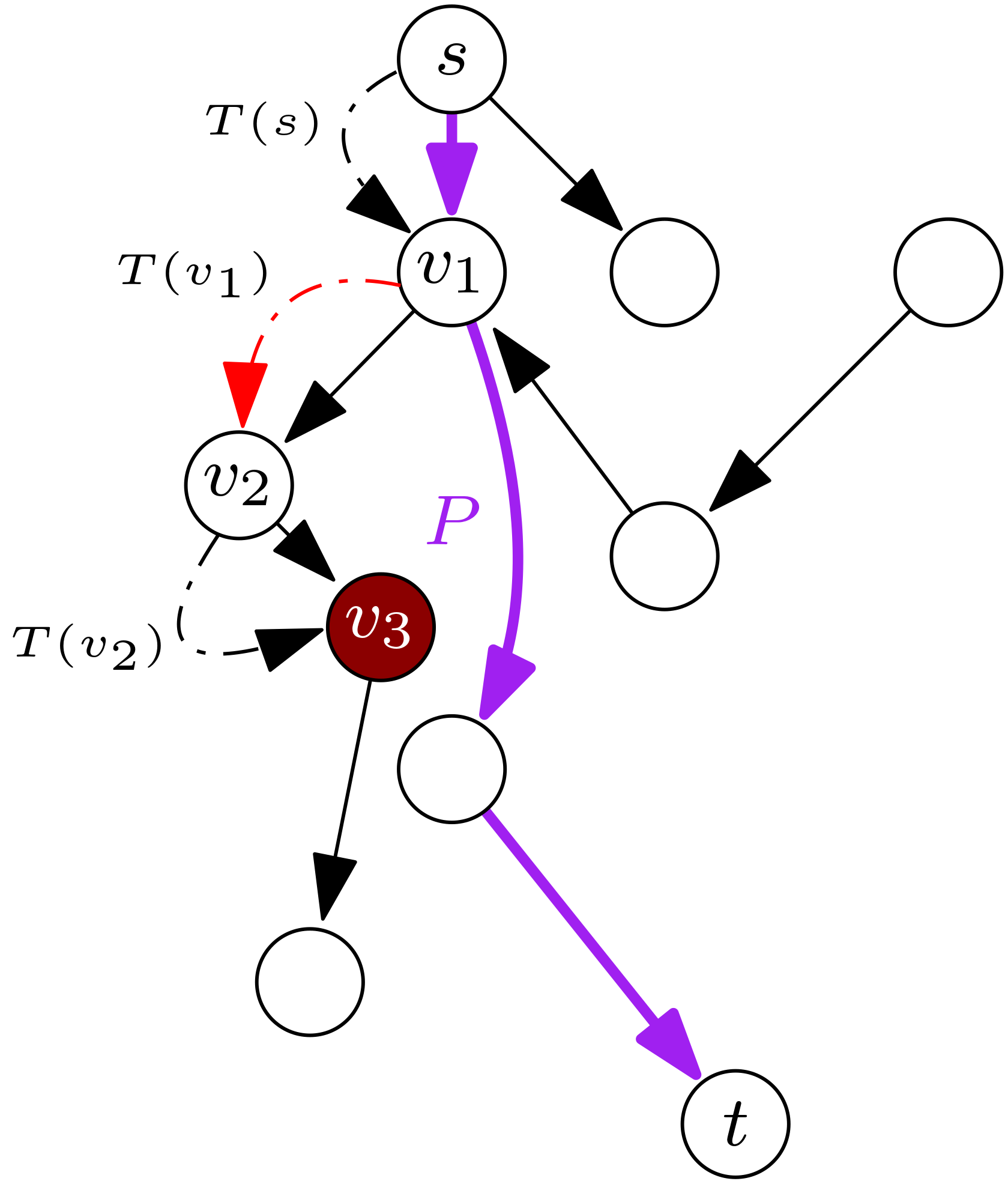
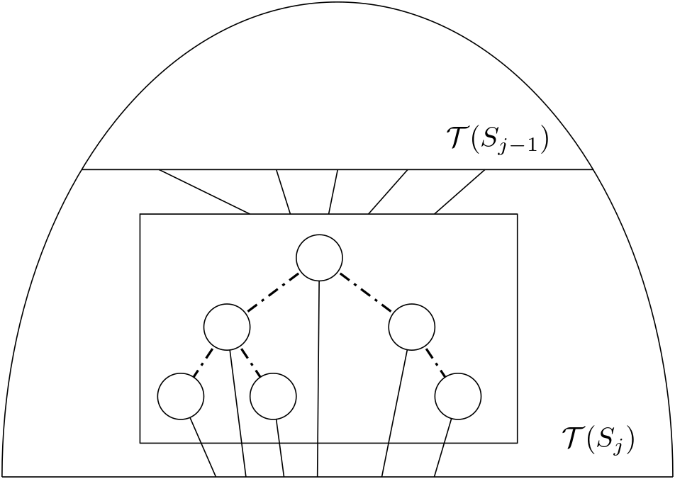
In this section, we provide an analysis tool that we use repeatedly in this paper and which may be of independent interest (e.g., to analyze randomized routing protocols). Specifically, we introduce path-guided pushdown random walks, which are related to biased random walks on a graph (e.g., see [5, 17]) and generalize the noisy binary search problem [15, 18]. See Figure 1 for a depiction of path-guided pushdown random walks.
A path-guided pushdown random walk is defined in terms of a directed acyclic graph (DAG), , that has a starting vertex, , a target vertex, , and a path, , from to , in (we assume ). We start our walk from the start vertex, , and we use a stack, , which initially contains only , and a transition oracle, , to determine our walk. For each vertex, , during our walk, we consult the transition oracle, , which first tells us whether and if so, then tells us the next vertex in to visit to make progress towards . can return , which means we should stay at , e.g., if .
Our model allows to “lie.” We assume a fixed error probability,222The threshold of simplifies our proof. We can tolerate any higher error probability bounded below , by repeating any query a constant number of times and taking the majority answer. , such that gives the correct answer with probability , independently each time we query . With probability , can lie, i.e., can indicate “” when , can indicate “” when , or can return a “next” vertex that is not an actual next vertex in (including returning itself even though ). Importantly, this next vertex must be an outgoing neighbor of . This allows us to maintain the invariant that holds an actual path in (with repeated vertices). Our traversal step, for current vertex , is as follows:
-
If indicates that (and ), then we set , which may be again, for the next iteration. This is a backtracking step.
-
If indicates that , then let be the vertex indicated by as next in , such that or is an edge in .333 If and is not an edge in , we immediately reject this call to and repeat the call to .
-
–
If , then we call and repeat the iteration with this same , since this is evidence we have reached the target, .
-
–
Else () if , then we set . That is, in this case, we don’t immediately transition to , but we take this as evidence that we should not stay at , as we did in the previous iteration. This is another type of backtracking step.
-
–
Otherwise, we call and set for the next iteration.
-
–
We repeat this step until we are confident we can stop, which occurs when enough copies of the same vertex occur at the top of the stack.
Theorem 1.
Given an error tolerance, for , and a DAG, , with a path, , from a vertex, , to a distinct vertex, , the path-guided pushdown random walk in starting from will terminate at with probability at least after steps, for a transition oracle, , with error probability .
The proof of Theorem 1 can be found in Appendix A. In short, we show that each “good” action by can undo any “bad” action by . By applying a Chernoff bound, we then show that, w.h.p., we reach after steps and terminate after another steps. The requirement that be polynomially small is used to ensure that premature termination is unlikely. For the remainder of the paper, we assume that for some constant . A majority of the algorithms below invoke path-guided pushdown random walks at most times. Taking the union bound over all invocations still shows that path-guided pushdown random walks fails with probability . Thus, for , all invocations succeed w.h.p. This choice of adds to the time for each walk. However, in our applications it can be shown that , so this does not change the asymptotic complexity of the operation.
4 Noisy Randomized Incremental Construction for Trapezoidal Maps
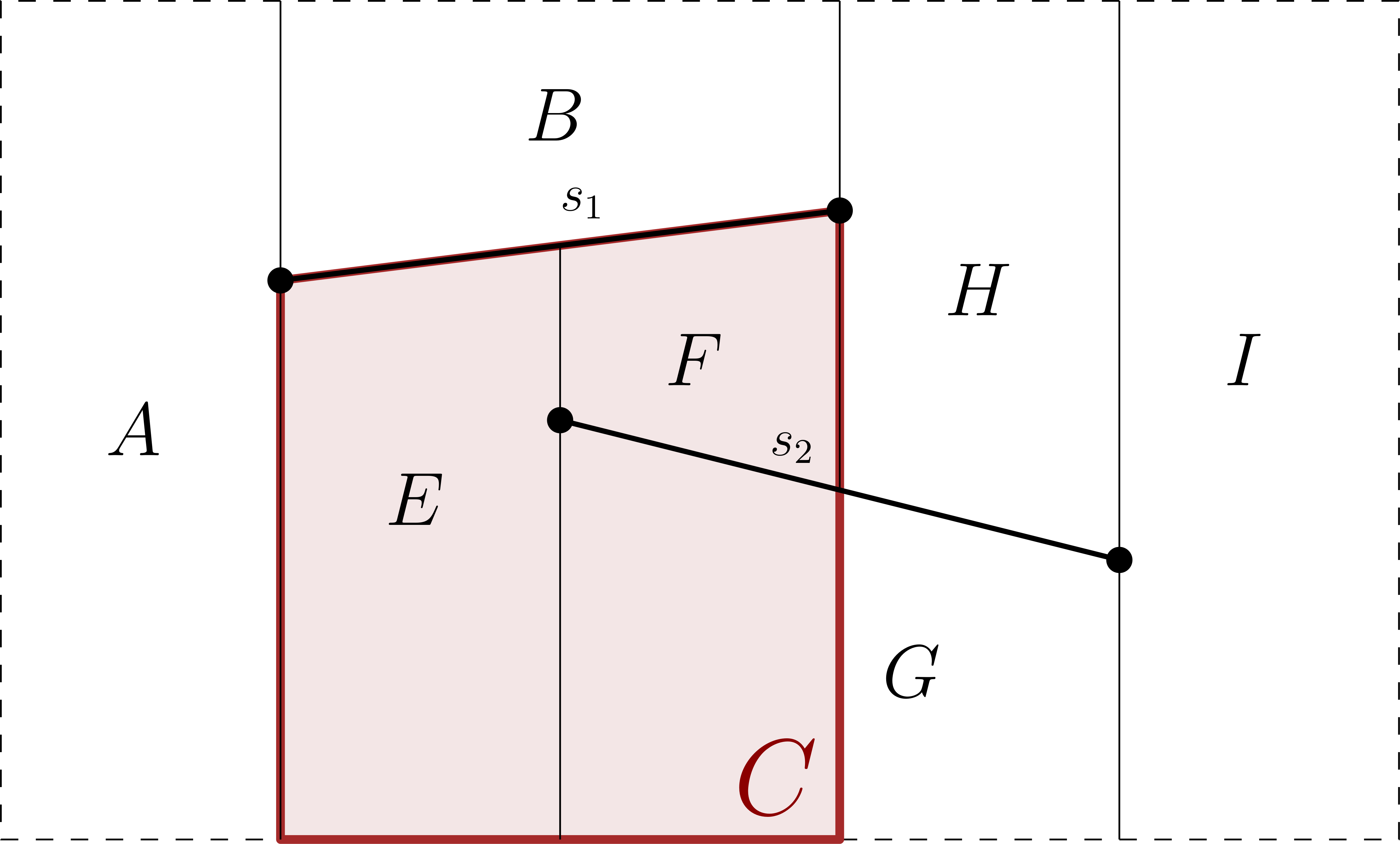
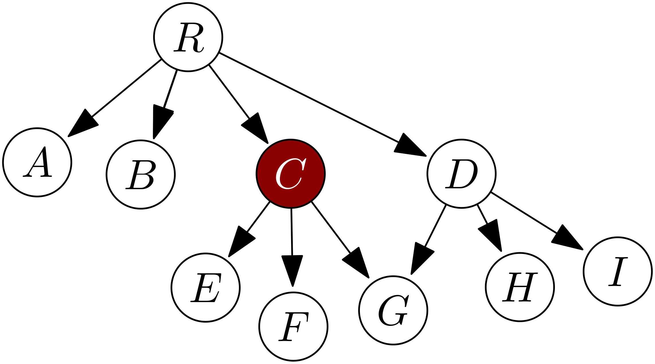
In this section, we show how a history DAG in a randomized incremental construction (RIC) algorithm can be used as the DAG of Theorem 1. Suppose we are given a set of non-crossing line segments in the plane and wish to construct their trapezoidal decomposition, . We outline below how the history DAG for a (non-noisy) RIC algorithm for constructing can be used as the DAG of Theorem 1. We show that, even in the noisy setting, such a DAG can perform point location in the history of trapezoids created and/or destroyed within the algorithm to locate the endpoints of successively inserted line segments. In particular, we consider a history DAG where any trapezoid destroyed in a given iteration points to the new trapezoids that replace it. This is in contrast to another variant of a history DAG that represents the segments themselves as nodes in the DAG [8], which seems less usable when primitives are noisy. To make our RIC algorithm noise-tolerant, we must solve two issues. The first is to navigate the history DAG in time w.h.p.; the second is to walk along each segment to merge and destroy trapezoids when it is added.
To navigate down the history DAG, we apply a path-guided pushdown random walk. To do so we must test, with a constant number of operations, whether we are on the path that a non-noisy algorithm would search to find the query endpoint of a new segment, . See Figure 2 for an example of this process. Each node of our history DAG represents a trapezoid (either destroyed if an internal node or current if a leaf node). Importantly, each of the at most four children of a node cover the parent’s trapezoid, but do not overlap. Therefore, we can define a unique path, w.r.t query , to be a sequence of trapezoids beginning at the root of the history DAG and ending at the leaf-node trapezoid containing . Each node on the path is the unique child of the previous node that contains . Thus, all our transition oracle must do to determine if we are on the correct path is to check whether is contained by the trapezoid mapped to our current node . If this test succeeds, the oracle determines (rightly or wrongly) that is on a valid path, and it proceeds to compare against the segment whose addition split trapezoid in order to return the next node of the walk. If one or more of these tests fails, the oracle says that is not on a valid path. Let be the sum of the lengths of the two unique paths corresponding to the endpoints of . If we set our error probability for path-guided pushdown random walks to be w.h.p. in , the point-location cost to insert the th segment is .
For the second issue, suppose there are trapezoids between the left and right endpoint of the th segment to be inserted, and that we need to walk left-to-right in the current subdivision to find them. To find the next trapezoid in this walk, we simply test if the segment endpoint that defines the right boundary of the current trapezoid lies above or below segment , e.g., determining whether to choose its upper-right or lower-right neighbor. Combining this above-below test with the trivial repetition strategy from Section 2, we can compute the correct sequence of trapezoids in time w.h.p.
Via the standard backwards analysis, and in expectation [8]. It has been shown [8, 38] that the search depth of the final history DAG is w.h.p. Therefore, after constructing the decomposition, we can use path-guided pushdown random walks to answer planar point-location queries in time w.h.p. We conclude the following.
Theorem 2.
We can successfully compute a trapezoidal decomposition map of non-crossing line segments w.h.p. in expected time, even with noisy primitives, and thereby construct a data structure (the history DAG) that answers point location queries in time w.h.p.
It is natural to hope that this can be extended to line segment arrangements with crossings, for which the best non-noisy time bounds are , achieved with a similar randomized incremental approach. We show in the full version that an extra logarithmic factor may be necessary, however.
5 Plane-Sweep Algorithms
In this section, we show that many plane-sweep algorithms can be adapted to our noisy-primitive model.
5.1 Noisy Balanced Binary Search Trees
We begin by noting that we can implement binary search trees storing geometric objects to support searches and updates in time w.h.p. by adapting the noisy balanced binary search trees recently developed for numbers in quantum applications by Khadiev, Savelyev, Ziatdinov, and Melnikov [24] to our noisy-primitive framework for geometric objects. Plane-sweep algorithms require us to store an ordered sequence of events that are visited by the sweep-line throughout the course of the algorithm while maintaining an active set of geometric objects for the sweep line in a balanced binary tree. Some plane-sweep algorithms, such as the one of Lee and Preparata that divides a polygon into monotone pieces [26], have a static set of events that can simply be maintained as a sorted array that is constructed using an existing noisy sorting algorithm [15]. Others, however, add or change events to the event queue as the algorithm progresses. In addition, the algorithms must also maintain already-processed data in a way that allows for new data swept over to be efficiently incorporated. The two most common dynamic data structures in plane-sweep algorithms are dynamic binary search trees and priority queues. Throughout this section, noise is associated with the comparison “?” where and are geometric objects.
Once a data structure is built, its underlying structure can be manipulated without noise. For example, we need no knowledge of the values held in a tree to recognize that it is imbalanced and to perform a rotation, allowing implementation of self-balancing binary search trees. For example, Khadiev, Savelyev, Ziatdinov, and Melnikov [24] show how to implement red-black trees [21] in the noisy comparison model for numbers. We observe here that the same method can be used for ordered geometric objects compared with noisy geometric primitives, with a binary search tree serving as the search DAG and a root-to-leaf search path as the path. See Appendix B for an explanation for how to instantiate path-guided pushdown random walks on a binary search tree.
5.2 Noisy Trapezoidal Decomposition with Segment Crossings
We can implement an event queue as a balanced binary search tree with a pointer to the smallest element to perform priority queue operations in the noisy setting.
Theorem 3.
Given a set, , of -monotone pseudo-segments444A set of -monotone psuedo-segments is a set of -monotone curve segments that do not self-intersect and such that any two of them intersect at most once [7, 1]. in the plane, we can construct a trapezoidal map of in time w.h.p., where is the number of pairs of crossing segments, even with noisy primitive operations.
Proof.
Bentley and Ottmann [6] compute a trapezoidal map of line segments via a now well-known plane-sweep algorithm, which translates directly to -monotone pseudo-segments. Pseudo-segment endpoints and intersection points are kept in an event queue ordered by -coordinates and line segments intersecting the sweep line are kept in a balanced binary search tree, both of which can be implemented to support searches and updates in time w.h.p. in the noisy model, as described above. Given the -time performance of the Bentley-Ottmann algorithm, this implies that we can construct the trapezoidal map of in time w.h.p.
We note that this running time matches the construction time in Theorem 2 for non-crossing line segments, but it does not give us a point-location data structure as in Theorem 2. Further, the upper bound of Theorem 3 is optimal with noisy primitive operations for via a reduction from computing line arrangements to computing trapezoidal decompositions. We show in the full version that computing an arrangement of lines in the noisy setting takes time.
5.3 Noisy Closest Pair
Here, we present another plane-sweep application in the noisy setting.
Theorem 4.
We can find a closest pair of points, from points in the plane, with noisy primitives, in time w.h.p.
Proof.
Hinrichs, Nievergelt, and Schorn show how to find a pair of closest points in the plane in time [22] by sorting the points by their -coordinate and then plane-sweeping the points in that order. They maintain the minimum distance seen so far, and a -table of active points. A point is active if has been processed and its -coordinate is within of the current point; once this condition stops being true, it is removed from the -table. The -table may be implemented using a balanced binary tree. When a point is processed, the -table is updated to remove points that have stopped being active, by checking the previously-active points sequentially according to the sorted order until finding a point that remains active. The new point is inserted into the -table, and a bounded number of its nearby points in the table are selected. The distances between the new point and these selected points are compared to , and is updated if a smaller distance is found.
In our noisy model, sorting the points takes time w.h.p. [15]. Checking whether a point has stopped being active and is ready to be removed from the -table may be done using the trivial repetition strategy of Section 2; its removal is a non-noisy operation. Inserting each point into the -table takes time w.h.p. Selecting a fixed number of nearby neighbors is a non-noisy operation, and comparing their distances to may be done using the trivial repetition strategy with a noisy primitive that compares two distances determined by two pairs of points. In this way, we perform work for each point when it is processed, and work again later when it is removed from the -table. Overall, the time is w.h.p.
We give this result mostly as a demonstration for performing plane sweep in the noisy model, since a closest pair (or all nearest neighbors) may be found by constructing the Delaunay triangulation (Section 7) and then performing min-finding operations on its edges.
An algorithm by Rabin [36] finds 2D closest points in time, beating the plane sweep implementation that our solution is based on, in a model of computation allowing integer rounding of numerical values derived from input coordinates. However, computing the minimum of elements takes time for noisy comparison trees [15], and Rabin’s algorithm includes steps that find the minimum among distances, so it is not faster than our algorithm in our noisy model. In the full version, we prove that if data is accessed only through noisy primitives that combine information from data points (allowing integer rounding), then finding the closest pair w.h.p. requires time . Thus, the plane-sweep closest-pair algorithm is optimal in this model.
6 Convex Hulls
In this section, we describe algorithms for constructing convex hulls that can tolerate probabilistically noisy primitive operations. Here, primitive operations are orientation tests and visibility tests for 2D and 3D convex hulls respectively. Sorting is also used throughout, so comparing the or coordinates of two points is also a noisy primitive.
6.1 Static Convex Hulls in 2D
We begin by observing that it is easy to construct two-dimensional convex hulls in time w.h.p. Namely, we simply sort the points using a noise-tolerant sorting algorithm [15] and then run Graham scan [8]. The Graham scan phase of the algorithm uses calls to primitives, so we can simply use the trivial repetition strategy from Section 2 to implement this phase in time w.h.p. We note that this is the best possible, however, since just computing the minimum or maximum of values has an -time lower bound for a high-probability bound in the noisy primitive model [15].
6.2 Dynamic Convex Hulls in 2D
Overmars and van Leeuwen [32] show how to maintain a dynamic 2D convex hull with insertion and deletion times, query time, and space. They maintain a binary search tree, , of points stored in the leaves ordered by -coordinates and augment each internal node with a representation of half the convex hull of the points in that subtree. They define an -hull of as the convex hull of , which is the left half of the hull of (-hull is defined symmetrically). It is easy to see that performing the same query on both the - and -hull of allows us to determine if a query point is inside, outside, or on the complete convex hull. We follow this same approach, showing how their approach can be implemented in the noisy-primitive model using path-guided pushdown random walks.
Overmars and van Leeuwen show that two -hulls and separated by a horizontal line can be merged in time. Rather than being a single binary search, however, their method involves a joint binary search on the two trees that represent and with the aim of finding a tangent line that joins them. At each step, we follow one of ten cases to determine how to navigate the trees of and/or . Because each decision may only advance in one tree, noisy binary search is not sufficient. Fortunately, as we show, the path-guided pushdown random walk framework is powerful enough to solve this problem in the noisy model. The challenge, of course, is to define an appropriate transition oracle. Say that the transition oracle has the ability to identify which case corresponds to our current position in and . This decision determines which direction to navigate in and/or and corresponds to choosing a child to navigate down an implicit decision DAG wherein each node has ten children. It remains to show how a transition oracle acting truthfully can determine if we are on the correct path.
We have each node of and maintain and pointers as described in Appendix B. The values at and are ancestors of whose keys are just smaller and just larger than respectively. They determine the interval of possible values of any node in ’s subtree, which corresponds to an interval of points on each hull. See Figure 3 for an example.
Say we are currently at node and node . We can perform four case comparisons: with , with , with , and with . Each outputs a region of and that the two tangent points must be located in. If the intersection of all four case comparisons contains the regions bounded by and as well as and , then we are on a valid path by the correctness of Overmars and van Leeuwen’s case analysis [32]. Since the noise-free process takes time, with a path-guided pushdown random walk using the transition oracle described above, this process takes time w.h.p.
To query a hull, we can perform noisy binary search on the - and -hull structures using the transition oracle of Appendix B. Updating the convex hull utilizes the technical lemma discussed above along with split and join operations on binary search trees [32]. We conclude the following.
Theorem 5.
We can insert and delete points in a planar convex hull in time per update w.h.p., even with noisy primitives.
6.3 Convex Hulls in 3D
In this section, we show how to construct 3D convex hulls in time w.h.p. even with noisy primitive operations. The main challenges in this case are first to define an appropriate algorithm in the noise-free model and then define a good transition oracle for such an algorithm. For example, it does not seem possible to efficiently implement the divide-and-conquer algorithm of Preparata and Hong [35] in the noisy primitive model as each combine step performs primitive operations. We begin by constructing a tetrahedron through any four points; we need the orientation of these four points, which can be found by the trivial repetition strategy in time. The points within this tetrahedron can be discarded, again using the trivial repetition strategy in time per point.
The main challenge to designing a transition oracle for the history DAG in this method is its nested nature. We have the nodes in the DAG themselves representing facets and pointing to the facets that replaced them when they were deleted. We also have the radial search structures, which maintain the set of new facets produced in a given iteration in sorted clockwise order around the point that generated them. See Figure 4 for a depiction of this.
Our transition oracle needs to be able to determine if we are on the correct path. Say we are given a query point, , being inserted in the th iteration of the RIC algorithm and are at node of the history DAG. To see if we are performing the right radial search, we first check if the ray from the origin to passes through ’s parent (in the history DAG, not the radial search structure). Then we must determine if we are performing radial search correctly. To do so, we can augment the radial search tree as described in Appendix B and perform two more orientation tests to determine if is on the right path in our current radial search structure. If a comparison returns false, then we use our stack to backtrack up the radial search structure or, if we are at its root, back to the parent node in the history DAG and its respective radial search tree. Thus, in just three comparisons, we can determine if we are on the right path in the history DAG. Similar to our trapezoidal decomposition analysis, we observe that the point-location cost in each iteration is , where is the length of the unique path in the history DAG corresponding to our query . An analysis by Mulmuley [31] shows that, over all iterations, in expectation. As a result, total point-location cost is in expectation.
Once a conflicting facet is found through the random walk, we can again walk around the hull and perform the trivial repetition strategy of Section 2 to determine the set of all conflicting facets, , in time. Each facet must be created before it is destroyed, so is upper-bounded by the total size of the history DAG. The same analysis by Mulmuley [31] shows that the expected size of the history DAG is . We conclude the following.
Theorem 6.
We can successfully compute a 3D convex hull of points w.h.p. in expected time, even with noisy primitives.
7 Delaunay Triangulations and Voronoi Diagrams
In this section, we describe an algorithm that computes the Delaunay triangulation (DT) of a set of points in the plane in the noisy-primitives model. Noise is associated with determining whether a point lies within some triangle and whether a point lies in the circle defined by some Delaunay edge . Here, we describe the algorithm under the Euclidean metric. In the full version, we show how to generalize our algorithm for other metrics.
Once again, we use a history DAG RIC similar to what we described in the previous section. This time, each node in the DAG represents the triangles that exist throughout the construction of the triangulation (see [31] for details). A leaf node is a triangle that exists in the current version, and an internal node is a triangle that was destroyed in a previous iteration. When we wish to insert a new point , we first use the history DAG to locate where is in the current DT. If is within a triangle , we split into three triangles and add them as children of . Otherwise is on some edge , and we split the two adjacent triangles and into two triangles each. Once this is done, we repeatedly flip edges that violate the empty circle property so that the triangulation becomes a DT again (see [8] Chapter 9.3). As described in [31], we store the new triangles in a radial search structure sorted CCW around the added point . Using a path-guided pushdown random walk in the history DAG to find the triangle containing is broadly similar to the process used to find conflicting faces in the 3D convex hull RIC. Once again, we use the ray-shooting and radial search queries described in Section 6.3. With a similar transition oracle to 3D convex hulls, we can determine where is in the current DT in time, where is the length of ’s unique path in the history DAG. Unlike for 3D convex hulls, there is a unique triangle or edge that is in conflict with , which simplifies the process of determining a unique path through the history DAG. We observe that if is not located in the triangle represented by the current node in the DAG, then we are not on the right path. Once we have found the triangle containing and added in new edges, we begin edge flipping. Using the trivial repetition strategy, each empty circle test costs time. The number of empty circle tests is proportional to the number of edges flipped, which is less than the total number of triangles created throughout the algorithm. Once again, Mulmuley’s [31] analysis shows that in expectation and the number of empty circle tests needed to update the DAG after point-location is in expectation. We conclude the following.
Theorem 7.
We can successfully compute a Delaunay triangulation of points w.h.p. in expected time, even with noisy primitives.
We remark that this also leads to an algorithm for constructing a Euclidean minimum spanning tree, in which we construct the Delaunay triangulation, apply a noisy sorting algorithm to its edge lengths, and then (with no more need for noisy primitives) apply Kruskal’s algorithm to the sorted edge sequence. In the following section, we generalize our Delaunay triangulation algorithm to work for a wider class of metrics, including all metrics for .
7.1 Generalized Delaunay Triangulations
In this section, we show the following:
Theorem 8.
Given points in the plane, we can successfully compute a generalized Delaunay triangulation generated by homothets of any smooth shape w.h.p. in expected time , even with noisy primitives.
A shape Delaunay tessellation is a generalization of a Delaunay triangulation first defined by Drysdale [12]. Rather than a circle, we instantiate some convex compact set in and redefine the empty circle property on an edge like so: given a set of points and some shape , the edge exists in the shape Delaunay tessellation iff there exists some homothet of with and on its boundary that contains no other points of [4]. We will consider smooth shapes, as arbitrary non-smooth shapes may cause to not be a triangulation under certain point sets [4]. Note that all metrics for correspond to smooth shapes (rather than a unit circle, they are unit rounded squares) and furthermore, all smooth shapes produce triangulations of the convex hull of [4, 39]. Similar to above, we use the general position assumption that no four points lie on a homothet of .
After inserting a point, , in the incremental algorithm, we draw new edges that connect to the points that comprise the triangle(s) that landed in. These new edges are Delaunay as either they are fully enclosed by the homothets of that covered the triangle(s) was located in or they are enclosed by the union of previously-empty shapes that covered each edge of the triangles. After this, the algorithm finds adjacent edges, tests if they obey the empty shape property, and flips them if not. In Theorem 3 of a work by Aurenhammer and Paulini [4], the authors prove that for any convex shape , local Delaunay flips lead to by showing that there exists some lexicographical ordering to these triangulations similar to how the Delaunay triangulation in maximizes the minimum angle over all triangles. Thus, the flipping algorithm used after an incremental insertion will terminate at a triangulation that is , where is the set .
Because the flipping process works as before, the point location structure can be easily adapted to this setting. As stated above, using a smooth shape guarantees that is an actual triangulation as opposed to a tree. Thus, in every iteration, there exists a triangle that the new point is enclosed by. The history DAG data structure is agnostic to the specific edge flips being made during the course of the algorithm and so works as expected. Our transition oracle also behaves the same.
In the Euclidean case, the backwards analysis of [8] uses the fact that a Delaunay triangulation of points has edges, any new triangle created in iteration is incident to the newly inserted point , and triangles are defined by at most three points. By planarity and by construction of the algorithm, all three hold true in this generalized case. Thus, we have the desired result.
8 Discussion
We have shown that a large variety of computational geometry algorithms can be implemented in optimal time or, for dynamic 2D hull, in time that matches the original work’s complexity with high probability in the noisy comparison model. We believe that this is the first work that adapts the techniques of noisy sorting and searching to the classic algorithms of computational geometry, and we hope that it inspires work in other settings, such as graph algorithms.
References
- [1] Pankaj K Agarwal and Micha Sharir. Pseudo-line arrangements: Duality, algorithms, and applications. SIAM Journal on Computing, 34(3):526–552, 2005. doi:10.1137/S0097539703433900.
- [2] Jonathan Allcock, Jinge Bao, Aleksandrs Belovs, Troy Lee, and Miklos Santha. On the quantum time complexity of divide and conquer, 2023. doi:10.48550/arXiv.2311.16401.
- [3] Andris Ambainis and Nikita Larka. Quantum algorithms for computational geometry problems. arXiv preprint arXiv:2004.08949, 2020. arXiv:2004.08949.
- [4] Franz Aurenhammer and Günter Paulini. On shape Delaunay tessellations. Inf. Process. Lett., 114(10):535–541, 2014. doi:10.1016/j.ipl.2014.04.007.
- [5] Yossi Azar, Andrei Z. Broder, Anna R. Karlin, Nathan Linial, and Steven Phillips. Biased random walks. Combinatorica, 16(1):1–18, 1996. doi:10.1007/BF01300124.
- [6] Jon L. Bentley and Thomas A. Ottmann. Algorithms for reporting and counting geometric intersections. IEEE Transactions on Computers, 100(9):643–647, 1979. doi:10.1109/TC.1979.1675432.
- [7] Chan. On levels in arrangements of curves. Discrete & Computational Geometry, 29:375–393, 2003. doi:10.1007/S00454-002-2840-2.
- [8] Mark de Berg, Marc van Kreveld, Mark Overmars, and Otfried Schwarzkopf. Computational Geometry: Algorithms and Applications. Springer, 3rd edition, 2008.
- [9] Dariusz Dereniowski, Aleksander Lukasiewicz, and Przemyslaw Uznanski. Noisy searching: Simple, fast and correct, 2023. arXiv:2107.05753.
- [10] Dariusz Dereniowski, Stefan Tiegel, Przemyslaw Uznanski, and Daniel Wolleb-Graf. A framework for searching in graphs in the presence of errors. In Jeremy T. Fineman and Michael Mitzenmacher, editors, 2nd Symp. on Simplicity in Algorithms (SOSA), volume 69, pages 4:1–4:17, 2019. doi:10.4230/OASICS.SOSA.2019.4.
- [11] Michael Dillencourt, Michael T. Goodrich, and Michael Mitzenmacher. Leveraging parameterized Chernoff bounds for simplified algorithm analyses. Inf. Process. Lett., 187:106516, 2025. doi:10.1016/j.ipl.2024.106516.
- [12] Robert L. (Scot) Drysdale, III. A practical algorithm for computing the Delaunay triangulation for convex distance functions. In David S. Johnson, editor, ACM-SIAM Symp. on Discrete Algorithms (SODA), 1990. URL: http://dl.acm.org/citation.cfm?id=320176.320194.
- [13] Herbert Edelsbrunner and Ernst Peter Mücke. Simulation of simplicity: a technique to cope with degenerate cases in geometric algorithms. ACM Trans. Graphics, 9(1):66–104, 1990. doi:10.1145/77635.77639.
- [14] Ehsan Emamjomeh-Zadeh, David Kempe, and Vikrant Singhal. Deterministic and probabilistic binary search in graphs. In Daniel Wichs and Yishay Mansour, editors, 48th ACM Symp. on Theory of Computing (STOC), pages 519–532, 2016. doi:10.1145/2897518.2897656.
- [15] Uriel Feige, Prabhakar Raghavan, David Peleg, and Eli Upfal. Computing with noisy information. SIAM J. Comput., 23(5):1001–1018, 1994. doi:10.1137/S0097539791195877.
- [16] Steven Fortune and Christopher J Van Wyk. Static analysis yields efficient exact integer arithmetic for computational geometry. ACM Trans. Graphics, 15(3):223–248, 1996. doi:10.1145/231731.231735.
- [17] Agata Fronczak and Piotr Fronczak. Biased random walks in complex networks: The role of local navigation rules. Phys. Rev. E, 80(1):016107, 2009. doi:10.1103/PhysRevE.80.016107.
- [18] Barbara Geissmann, Stefano Leucci, Chih-Hung Liu, and Paolo Penna. Optimal sorting with persistent comparison errors. In Michael A. Bender, Ola Svensson, and Grzegorz Herman, editors, 27th European Symp. on Algorithms (ESA), volume 144 of LIPIcs, pages 49:1–49:14, 2019. doi:10.4230/LIPICS.ESA.2019.49.
- [19] Benoît Groz, Frederik Mallmann-Trenn, Claire Mathieu, and Victor Verdugo. Skyline computation with noisy comparisons. In Leszek Gasieniec, Ralf Klasing, and Tomasz Radzik, editors, Combinatorial Algorithms, pages 289–303, Cham, 2020. Springer. doi:10.1007/978-3-030-48966-3_22.
- [20] Joachim Gudmundsson and Martin P. Seybold. A tail estimate with exponential decay for the randomized incremental construction of search structures. In Joseph (Seffi) Naor and Niv Buchbinder, editors, ACM-SIAM Symp. on Discrete Algorithms (SODA), pages 610–626, 2022. doi:10.1137/1.9781611977073.28.
- [21] Leonidas J. Guibas and Robert Sedgewick. A dichromatic framework for balanced trees. In 19th IEEE Symp. on Foundations of Computer Science (FOCS), pages 8–21, 1978. doi:10.1109/SFCS.1978.3.
- [22] Klaus Hinrichs, Jürg Nievergelt, and Peter Schorn. Plane-sweep solves the closest pair problem elegantly. Inf. Process. Lett., 26(5):255–261, 1988. doi:10.1016/0020-0190(88)90150-0.
- [23] Kazuo Iwama, Rudy Raymond, and Shigeru Yamashita. General bounds for quantum biased oracles. IPSJ Digital Courier, 1:415–425, 2005. doi:10.2197/ipsjdc.1.415.
- [24] Kamil Khadiev, Nikita Savelyev, Mansur Ziatdinov, and Denis Melnikov. Noisy tree data structures and quantum applications. Mathematics, 11(22), 2023. doi:10.3390/math11224707.
- [25] Rolf Klein, Rainer Penninger, Christian Sohler, and David P. Woodruff. Tolerant algorithms. In Camil Demetrescu and Magnús M. Halldórsson, editors, 19th European Symp. on Algorithms (ESA), volume 6942 of LNCS, pages 736–747. Springer, 2011. doi:10.1007/978-3-642-23719-5_62.
- [26] D. T. Lee and F. P. Preparata. Location of a point in a planar subdivision and its applications. SIAM J. Comput., 6(3):594–606, 1977. doi:10.1137/0206043.
- [27] Maarten Löffler. Data Imprecision in Computational Geometry. PhD thesis, Utrecht University, 2009.
- [28] Maarten Löffler and Jack Snoeyink. Delaunay triangulation of imprecise points in linear time after preprocessing. Comput. Geom., 43(3):234–242, 2010. doi:10.1016/j.comgeo.2008.12.007.
- [29] Kurt Mehlhorn, Ralf Osbild, and Michael Sagraloff. Reliable and efficient computational geometry via controlled perturbation. In Michele Bugliesi, Bart Preneel, Vladimiro Sassone, and Ingo Wegener, editors, Int. Colloq. Automata, Languages and Programming (ICALP), volume 4051 of LNCS, pages 299–310. Springer, 2006. doi:10.1007/11786986_27.
- [30] Kurt Mehlhorn and Stefan Schirra. Exact computation with leda_real – theory and geometric applications. In Götz Alefeld, Jiri Rohn, Siegfried M. Rump, and Tetsuro Yamamoto, editors, Symbolic Algebraic Methods and Verification Methods, pages 163–172. Springer, 2001. doi:10.1007/978-3-7091-6280-4_16.
- [31] Ketan Mulmuley. Computational Geometry: An Introduction Through Randomized Algorithms. Prentice Hall, 1994.
- [32] Mark H. Overmars and Jan van Leeuwen. Maintenance of configurations in the plane. J. Comput. System Sci., 23(2):166–204, 1981. doi:10.1016/0022-0000(81)90012-X.
- [33] Andrzej Pelc. Searching with known error probability. Theoret. Comput. Sci., 63(2):185–202, 1989. doi:10.1016/0304-3975(89)90077-7.
- [34] Andrzej Pelc. Searching games with errors—fifty years of coping with liars. Theoret. Comput. Sci., 270(1-2):71–109, 2002. doi:10.1016/S0304-3975(01)00303-6.
- [35] Franco P. Preparata and Se June Hong. Convex hulls of finite sets of points in two and three dimensions. Communications of the ACM, 20(2):87–93, 1977. doi:10.1145/359423.359430.
- [36] Michael O. Rabin. Probabilistic algorithms. In J. F. Traub, editor, Symp. New Directions in Algorithms and Complexity, pages 21–39. Academic Press, 1976.
- [37] Alfréd Rényi. On a problem in information theory. Magyar Tud. Akad. Mat. Kutató Int. Közl., 6:515–516, 1961.
- [38] Sandeep Sen. A unified approach to tail estimates for randomized incremental construction. In 36th International Symposium on Theoretical Aspects of Computer Science (STACS 2019), pages 58–1. Schloss Dagstuhl – Leibniz-Zentrum für Informatik, 2019.
- [39] Sven Skyum. A sweepline algorithm for generalized Delaunay triangulations. DAIMI Report Series, 20(373), 1991.
- [40] Emanuele Viola. The communication complexity of addition. Combinatorica, 35(6):703–747, 2015. doi:10.1007/s00493-014-3078-3.
- [41] Ziao Wang, Nadim Ghaddar, Banghua Zhu, and Lele Wang. Noisy sorting capacity. IEEE Transactions on Information Theory, 70(9):6121–6138, 2024. doi:10.1109/TIT.2024.3425281.
- [42] Chee-Keng Yap. Symbolic treatment of geometric degeneracies. J. Symbolic Comput., 10(3-4):349–370, 1990. doi:10.1016/S0747-7171(08)80069-7.
Appendix A Path-guided Pushdown Random Walks
A.1 Correctness and analysis
In this section we prove that w.h.p. the path-guided random walk terminates with the correct answer to its search problem (Theorem 1). To do so we first need to define a termination condition for the walk. It is not adequate to terminate merely after an appropriate number of steps: with constant probability, the final step of the walk will be taken after an erroneous oracle result, and may be incorrect. On the stack used to guide the algorithm, we store along with each vertex a repetition count, equal to one if the vertex is different from the previous vertex on the stack, and equal to the previous repetition count otherwise. We terminate the algorithm when this repetition count reaches an appropriately large value, .
Lemma 9.
If it does not terminate earlier, the path-guided random walk will reach the correct goal vertex , within steps, with high probability, with a constant factor determined by the analysis below.
Proof.
Define a call to the transition oracle, , in our random walk as “good” if it returns the correct answer (i.e., does not lie) and “bad” otherwise, so that each call is bad independently with probability at most . Note that if we are at a node, , and , then a good call with either undo a previous bad call to stay at or it will move to the next vertex in . Also, if we are already at , then a good call will keep us at , adding another copy of to the top of the stack, . Alternatively, if we are a node, , then a good call with either undo a previous bad call to stay at or it will move back to a previous node in our traversal, which undoes a previous bad call to move to . Moreover, if we repeat this latter case, we will eventually return back to a node in . Thus, every good call either undoes a previous bad call or makes progress towards the target vertex, . Admittedly, if we are at a node, , then a bad call can undo a previous good call (e.g., which was to move to or stay at if ). Also, a sequence of bad calls can even deviate from and return back to it – but because is a DAG, a series of bad calls cannot return back to a previously visited vertex of . Thus, a path-guided pushdown random walk will successfully reach the target vertex, , if the difference between the number of good calls and bad calls is at least , the length of the path, . Let be an indicator random variable that is iff the th call to the transition oracle is bad, and let . Since each call is bad independent of all other calls, we can apply a Chernoff bound to determine an upper bound on the probability that the difference between the number of good calls and bad calls is less than , i.e., if , that is, if . Further, note that . Then, for , the failure probability is
Further, by a Chernoff bound from Dillencourt, Goodrich, and Mitzenmacher [11] (Theorem 7),
This establishes the proof.
As mentioned above, the condition can, with the same asymptotic performance as in Theorem 1 be replaced with any error probability bounded away from . We caution, however, that while Theorem 1 provides a high-probability guarantee we reach the target vertex, , it does not provide a high-probability guarantee we visit every vertex of the path, . There is an exception to this, which we describe now.
Corollary 10.
If is a tree, then the path-guided pushdown random walk in will visit every node in .
Proof.
By definition, there is a unique path from the root of to the target vertex . Thus, according to Theorem 1, with high probability after steps, the path represented by the stack must equal the intended path , which also must equal .
Lemma 11.
If it does not terminate earlier, the path-guided pushdown random walk will accumulate copies of the goal vertex on its stack, after steps, and therefore terminate, with high probability.
Proof.
This follows by applying Lemma 9 to a modified DAG in which we expand each vertex of into a chain of copies , , , of with a repetition count, as used in the termination condition of the algorithm.
Lemma 12.
The path-guided pushdown random walk will not terminate with any other vertex than , with high probability.
Proof.
By another application of Chernoff bounds, and by the assumption that is polynomially small, the probability that the algorithm terminates at step with an incorrect vertex is itself polynomially small, with an exponent that can be made arbitrarily large (independent of our original choice of ) by an appropriate choice of the constant factor in the repetition count threshold used for the termination condition. By choosing this constant factor appropriately, we can make the probability of termination at any fixed step smaller than by a factor at least as large as the high-probability bound on the number of steps of the walk in Lemma 11. The result follows by applying the union bound to all the steps of the walk.
Proof of Theorem 1..
Termination of the algorithm w.h.p. follows from Lemma 11, and correctness once terminated follows from Lemma 12. For a given high-probability bound , we apply Lemma 11 and Lemma 12 with and then apply the union bound to get a bound on the probability that the algorithm terminates with a correct answer.
A.2 Counterexample to Generalizations
It is very tempting to consider a generalization of the path-guided pushdown random walk defined by a set of valid nodes and goal nodes, with the property that a non-noisy search starting from any valid node will reach a goal node and then stop. With a noisy oracle that determines whether a node is valid and if so follows a noisy version of the same search, one could hope that this generalized algorithm would quickly reach a goal state. The path-guided pushdown random walk would then be a special case where the valid nodes are exactly the nodes on the non-noisy search path from the root node. However, as we show in this section, this generalization does not work with the same fast high-probability termination bounds, unless additional assumptions are made (such as the assumptions giving the special case of the path-guided pushdown random walk).
Consider the following search problem: the DAG to be searched is simply a complete binary tree with height . One root-to-leaf path on this DAG is marked as valid, with the nodes on this path alternating between non-goal and goal nodes, so that the non-noisy search from the root stops after one step but other later stops would also produce a valid result. We have a noisy oracle with the following behavior:
-
At a leaf node of the binary tree, or an invalid node, it always produces the correct result.
-
At a valid non-leaf node, it follows the same behavior as a non-noisy oracle with probability : that is, it correctly identifies whether the node is a goal, and if not returns the unique valid child. With probability (for some suitably large constant ) it returns the valid child regardless of whether the node is a goal. And with the remaining probability it returns the invalid child.
Now consider the behavior on this problem of a path-guided random walk, as defined above with a repetition-count termination condition. It will follow the valid path in the binary tree, with brief diversions whenever the noisy oracle causes it to walk to a node not on the path. At any goal node, it will wait at that node, accumulating more repetitions of the node, until either it achieves repetitions (with a constant factor determined by the desired high probability bound) or the noisy oracle tells it to take one more step along the valid path. The probability of reaching repetitions without taking one more step is , and by adjusting relative to we can make this probability less than . With this choice, by the union bound, the random walk will eventually take one more step from each goal node until finally reaching the leaf goal node. The expected number of steps that it waits at each goal node will be , so the expected number of steps in the overall random walk, before reaching the leaf goal node and then accumulating enough repetitions to terminate, will be .
It also would not work to use a termination condition of making enough steps to have high probability of reaching a goal node, and then stopping. If this number of steps is not enough to reach the leaf goal node, the probability of stopping at a non-goal node would be too high.
Thus, without either a change of algorithm or more assumptions on the valid and goal node sets, this generalized random walk can be made to take a number of steps that is longer than by a non-constant factor.
Appendix B Transition Oracle for Binary Search Trees
While path-guided pushdown random walks applies to many DAGs, many fundamental computational geometry algorithms rely on binary search trees. In this appendix, we present a transition oracle for BSTs.
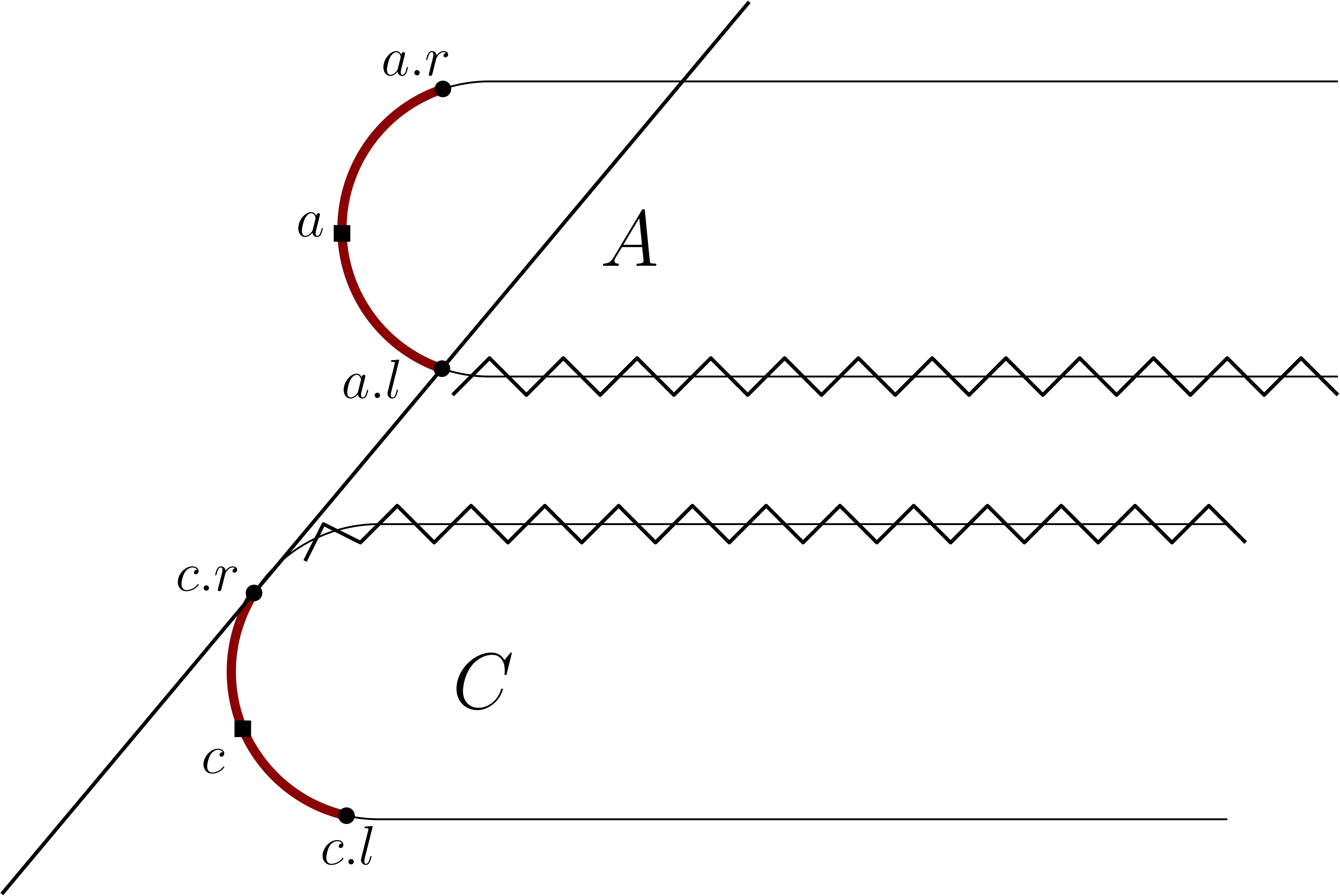
Say that we are attempting to find some value in a binary search tree . By properties of BSTs, there is a unique path from the root to the node containing . If there is no such node, there is still a unique path to the nonexistent leaf that would contain . When a call to the transition oracle is good, we expect it to correctly determine if we are on said valid path only using a constant number of comparisons. To do so, we add a constant amount of extra data to each node.
For each node of the BST, let be the unique path from the root to . Let be the lowest ancestor of whose right child is in (or a sentinel representing ). Likewise, let be the lowest ancestor of whose left child is in (or a sentinel representing ). One of is ’s parent. Observe that, if we have correctly navigated to , must be in between the values held by and . Thus, by adding two pointers to each node, the transition oracle can determine if we are on the correct path using two comparisons. See Figure 5 for a visual depiction of the pointers and and their effect. Augmenting the tree with these pointers can be done in extra time per insertion and deletion. With slight modification, we can also support inexact queries such as for predecessors or successors.
