Link Diameter, Radius and 2-Point Link Distance Queries in Polygonal Domains

Abstract
We show how to preprocess a polygonal domain with holes so that the link distance (the number of links in a minimum-link path) between two query points in the domain can be reported efficiently. Using our data structures, the link diameter of the domain (i.e., the maximum number of links that may be required in a minimum-link path between two points in the domain) as well as the link center and radius of the domain (i.e., the point minimizing the maximum link distance to the furthest point in the domain and this maximum link distance) can be found in polynomial time. We also give a simpler algorithm for finding the link diameter, not using the link distance query structures. Answering 2-point link distance queries and computing the link diameter/radius/center in polygonal domains have been open questions since these problems were studied for simple polygons in the 90’s.
Keywords and phrases:
Minimum-link paths, link distance, diameter, center, radius, 2-point distance queriesCopyright and License:
2012 ACM Subject Classification:
Theory of computation Design and analysis of algorithmsEditors:
Pat Morin and Eunjin OhSeries and Publisher:
1 Introduction
In computational geometry, the complexity of paths within polygonal domains is often measured not only by their length but also by their structural simplicity. This is particularly relevant in areas such as motion planning, robotics, and geographic information systems, where simplifying complexity can reduce computational overhead. A minimum-link (minlink) path between points in a polygonal domain is a polygonal - path with the minimum number of edges (links). The number of links in a minlink path is the link distance between and , providing such a measure of path complexity. The link diameter of is the maximum possible link distance between any two points in the domain. The link center of the domain is the point minimizing the maximum link distance to points of ; this maximum distance is the link radius. The above notions are analogous to the same concepts (diameter, center, radius) for arbitrary metric spaces.
1.1 On the complexity of computing optimal geometric paths
Both geodesic (shortest) and minlink paths may be more intricate than it feels from a glance:
-
It is folklore that geodesic paths may be found by searching the visibility graph of the domain; however, even if the vertices have integer coordinates, it is not known whether one can compare, in polynomial time, the length of a path to an integer – the length is the sum of square roots and no polynomial-time algorithm is known for comparing the sum to a number.
-
As explained in Section 2.1, vertices of a minlink path cannot always be snapped to a discrete set of points, leading to high bit complexity of the paths even in simple polygons [19, 21]. In a polygonal domain with holes, it is not immediately clear how to find a minlink path in polynomial time. One may compute the -link reachable regions, from the starting point, for increasing , but bounding the complexity of the regions (and hence the algorithm’s runtime) requires an insight [25].
The problems considered in this paper (2-point shortest path queries, diameter and radius) take the complexity to the next level. Quoting [5]: “no algorithm for computing the diameter and radius under the link distance is known, not even one that runs in exponential time.” In particular, nothing directly prevents the problems from being NP-hard or -hard. We show that the problems admit polynomial-time solutions. The running times are high: we leave the speed up as future work. (Note that there are plenty of algorithms with high running times that “just” show polynomiality of long-standing open problems; computational geometry examples range from a 20yr-old -time approximation algorithm [13] for covering an -gon with fewest convex subpolygons to a recent -time algorithm for star-partitioning a simple polygon[1].)
2 Preliminaries and related work
Let denote the number of vertices of . The visibility polygon (VP) of a point is the set of points in seen by . The weak visibility polygon of a subset is the union of the VPs of the points of ; equivalently, the weak visibility polygon is the set of points seen by at least one point of . The visibility graph (VG) of is the graph on vertices of , whose edges connect pairs of mutually visible vertices. We assume that edges of are also edges of the VG (i.e., that neighboring vertices of see each other along the boundary edge).
2.1 Link distance and bit complexity
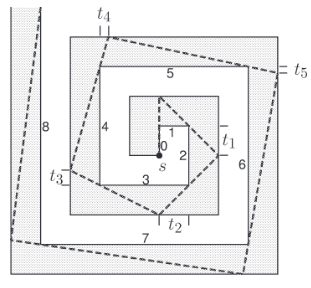
Computing the link diameter and radius/center of a polygonal domain with holes has been open since analogous problems were considered for simple polygons some 30 years ago [28, 4]. The reason why even an exponential-time solution is not obvious is because vertices of a minlink path do not necessarily lie on VG or some other discrete structure determined from the polygon (Fig. 1): it was shown [19, 21] that bits may be required to represent coordinates of vertices of the minlink path, even if the vertices of have integer coordinates specified with bits.
2.2 Staged illumination
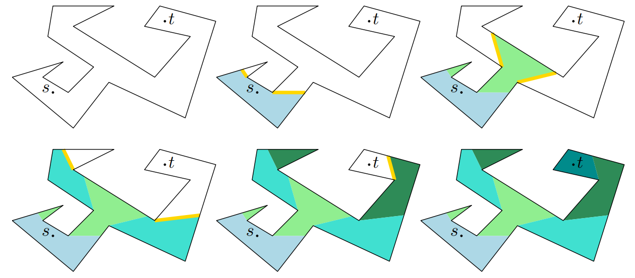
Algorithms for computing the link distance from a source point [26, 15, 17, 25] employ the “staged illumination” paradigm (see, e.g., the handbooks [23, Chapter 12] and [30, Chapter 31.3]): At the first stage, place the light source at and illuminate VP of – this is the set of points with link distance 1 from . At the beginning of any subsequent stage, the boundary between the lit and the dark portions of is defined by a set of line segments we call windows (any window starts at a vertex and ends on the boundary of ) which bound the weak visibility polygon of the area lit at the previous stage.
Figure 2 (left)t illustrates the staged illumination in a simple polygon. To efficiently run the staged illumination in a polygonal domain with holes [25], some chains of windows are replaced by their relative convex hulls within – essentially snapping windows to edges of VG. See Figure 2 (right) and [25], in particular, Figures 2–5 therein for the details.
The greedy path [22, 4] from to a window is the minlink path whose links are all aligned with windows and whose last link is aligned with . E.g., the path in Fig. 1 is greedy.

2.3 Distance map
The link distance map, denoted LDM(), from the source point is a decomposition of into cells such that the link distance from to any point within one cell is the same. Note that it is not required that the cells of LDM are maximal (i.e., that the link distance necessarily changes as you step from a cell to a neighboring cell): the only requirement is that the distance never changes within a cell.
For simple polygons, an LDM is really a by-product of the staged illumination (the edges of the map are the windows). Both a single minlink path and the LDM can be computed in time (because in a simple polygon the windows are pairwise disjoint, the LDM in it is also called a “window partition” [28, 4]).
In polygons with holes the LDMs can have ) complexity [29], and extra care must be taken in order to produce the LDM. In [25, Theorem 12] it was shown how to build the LDM in time, where notation suppresses polylogarithmic factors. The map is defined by an arrangement of windows (called “illumination edges” in [25]) within the domain.
Similarly to constructing an LDM from a point, one can build LDM from a source chord of (Fig. 3): the weak VP of is the set of points reachable with 1 link from , and the subsequent steps of the illumination are defined in the same way as for a point source. LDMs from segments were built already in early work [28] on link distance; in particular, LDMs from chords were used for finding the link center of a simple polygon [11].
2.4 1-point queries
After being preprocessed for point location, an LDM allows one to report the link distance from the source to a query point in optimal time, by locating the cell of the map that contains (enhanced with the backpointers, the map lets one report an actual minlink path in the additional time proportional to the number of links). An LDM is thus analogous to the shortest-path map (SPM()) in , which decomposes the domain into cells such that the length of the geodesic (shortest) path from to any point in one cell is given by the same formula. Note that while SPMs have linear complexity and can be built in linear (for simple polygons) or near-linear (for polygons with holes) time [34, 33], finding even a single minlink path in polygons with holes is 3SUM-hard [24] (an -time algorithm is given in [25]).
3 Prior work on 2-point queries and our results
While LDMs and SPMs give complete answers to the 1-point link and geodesic distance query resp. (for a fixed source, report the distance from a query point to the source), for the 2-point distance query problem (report the distance between two query points and ), the solutions achieving optimal query time are much more involved [32, 9, 16, 4, 10]:
-
An optimal (linear-preprocessing) algorithm is known only for 2-point geodesic distance queries in simple polygons [16].
-
A cubic-size data structure for link distance queries in simple polygons was given in [4].
-
For geodesic distance queries in polygonal domains, two methods were presented in [9]:
- 2d SPM equivalence decomposition
-
splits into (a polynomial number of) cells such that SPM() remains combinatorially the same (called “topologically equivalent” in [9, 7]) while stays within one cell, and stores a parametric SPM for each cell (the parameter being the location of within the cell: the parametric SPM records how the edges of SPM() change depending on where is). After preprocessing the parametric SPM for parametric point location [9, Section 4.2], 2-point geodesic distance queries may be answered by locating in the decomposition of and then locating in the parametric SPM().
- 4d geodesic distance equivalence decomposition
-
splits into (a polynomial number of) cells such that the geodesic distance between any pair of points (, ) within one cell is given by the same formula, i.e., by the same function of (, ). (On a detailed note, [9] presented two 4d structures: the vanilla -space 4d decomposition introduced in [9, Section 3] first, and the improved -size data structure in [9, Theorem 3.1] – we refer here to the former decomposition because the improved one, being specific to geodesic paths, does not work for us; similarly we did not see how to extend to link distance the recent data structure for geodesic paths from [10].)
-
No data structure for 2-point link distance queries in polygonal domains with holes has been known previously. One of the contributions of this paper is working out such data structures (analogous to the 2d and the 4d decomposition for geodesic queries [9]) by extending the solution of [4] (for 2-point link distance queries in simple polygons) to polygons with holes. Specifically, we provide the following two data structures:
- 2d LDM equivalence decomposition
-
is the decomposition of into (a polynomial number of) cells such that LDM() remains combinatorially the same while stays in one cell. The map, i.e., its vertices and edges (windows), is a known function of (the functions may be different in different cells, but within one cell the function is same).
- 4d link distance equivalence decomposition
-
decomposes into (a polynomial number of) cells such that the link distance between any pair (, ) in one cell is the same.
3.1 Diameter and radius/center
Computing the diameter and radius is intimately connected to the 2-point distance query structures, described above, via the following observation applicable to both geodesic and link distances – hence the prefix Meta:
MetaTheorem 1.
If the 2d map equivalence decomposition of or the 4d distance equivalence decomposition of can be built in polynomial time, then the diameter and the radius/center of can be computed in polynomial time.
Proof.
Go through every cell of the 2d map equivalence decomposition.
-
For the geodesic distance, the maximum distance from is attained at a vertex of SPM() [7, Lemma 1]. Since in every cell , it is known how SPM() changes with , distances from to all vertices are also known, and hence the maximum distance from to a point in is also known (from the upper envelope of the distances).
-
For the link distance, the maximum distance from is the distance to points in the cell of LDM() farthest from (any point in a cell of LDM() has the same link distance from – no need for the envelope).
To identify the diameter, take the maximum distance to the furthest point, and for the radius take the minmax; for the final answer, choose the best accordingly. To find the diameter, one may also go through every cell of the 4d decomposition and in every cell find the pair (, ) that maximizes the - distance – the diameter will be given by the overall maximum.
3.2 State of the art and our contribution
Solutions based on MetaTheorem 1 are not very efficient, and faster algorithms exist for finding both the geodesic diameter [6] and radius [31] of polygonal domains (in simple polygons, linear-time algorithms exist for both geodesic diameter [18] and radius [3]; link diameter [27] and radius [11] of simple polygons can be found in near-linear time). Existing results regarding diameter and radius are summarized in Table 1: essentially, the only case that has been missing is link distance in polygons with holes. Similarly, for simple polygons 2-point distance query data structures are known both for geodesic [16] and link distance [4], while for polygonal domains the problem has been solved only for the geodesic distance [9].
In this paper, we fill the gaps by showing how to construct the 2d map equivalence decomposition of a polygonal domain and the 4d distance equivalence decomposition of under the link distance. By MetaTheorem 1, this leads to polynomial-time algorithms for finding the link diameter and radius/center of the domains .
| simple polygon | polygonal domain | |||
|---|---|---|---|---|
| Diameter | Radius | Diameter | Radius | |
| Geodesic | [18] | [3] | Poly-time [6] | Poly-time[7, 31] |
| Link | [27] | [11, 20] | Poly-time [this paper] | |
The rest of the paper is organized as follows. Section 4 gives a simple algorithm to compute the link diameter (without resorting to MetaTheorem 1), and Section 5 presents data structures for 2-point link distance queries. Our data structures reuse, extend and combine the techniques of [4] (link distance queries in simple polygons) and [9] (geodesic distance queries in polygonal demands with holes): analogously to [9], our data structures are the 2d LDM equivalence decomposition and the 4d link distance equivalence decomposition. We conclude in Section 6 with some open problems.
4 A simple algorithm for link diameter
Throughout the paper, “distance” will mean link distance, “length” of an - path will mean the link distance between and along the path, etc. Slightly abusing the terminology, we will use the term diameter to mean both a minlink path between two diametrical endpoints and the number of links in such a path.
The idea of the algorithm in this section is that finding the diameter is easy if one of the following holds: the diameter is 1 or 2, a diameter endpoint is on a vertex, or a diameter edge is aligned with an edge of VG. The main structural observation is that we are always in one of the above-listed easy cases. The diameter is 1 if and only if is a convex polygon. The diameter is at most 2 if and only if for any there are rays from and which intersect each other before exiting the domain: the intersection point is the bend of a 2-link - path. We may rotate about , sliding along , until the link hits a vertex of (or until is on , but we assume that we deal with minlink paths only, so in particular it is not possible to decrease the number of links by rotating a link of the path). Thus, iff for any there are vertices and of , visible to and resp., such that the rays intersect, at a point , before exiting . We look at the question from the “other” side, i.e., from the point of view of and : we go through every pair of vertices and compute the set of pairs such that and may support the links of a 2-link - path. If the union of the sets , for all pairs , fully covers , then ; otherwise, there exist points , with link distance at least 3. To compute , we first of all decompose by extensions of VG edges: any point within one cell of the decomposition sees the same set of vertices; in particular, we consider only the cells from which both and are seen. As moves within such a cell , the rays rotate around resp., sweeping the locations for , resp. and thus creating – the subset of corresponding to having in . To implement the creation of , triangulate : the subset of obtained from in one triangle, has constant description complexity, and is the union of such subsets over all the triangles.
5 Two-point link distance queries
In this section we show how to compute the 2d LDM equivalence decomposition and the 4d link distance equivalence decomposition – the data structures for 2-point link distance queries, analogous to the structures of [9] for geodesic queries (see Section 3). Our data structures extend the data structure of [4] (for 2-point link distance queries in simple polygons) to polygonal domains with holes. The extension, allowing us to track combinatorial changes in LDM() for , is two-fold:
- Same windows.
-
In addition to decomposing the boundary of the polygon into “atomic segments” (as was done in [4]), we decompose the entire into “atomic cells” by overlaying LDMs from extensions of VG edges – for all in one cell of the decomposition, LDM() has the same set of windows. Moreover, the same subset of windows rotates as moves within , while the other windows, , are not influenced by the location of in the cell.
- Same arrangement of windows.
-
We track possible intersections among windows in LDM(), which may change because the rotating windows sweep through the domain as moves.
5.1 Extended visibility graph
For a line segment in let be the chord of containing (i.e., is extended maximally within ). Define the Extended Visibility Graph EVG = { is an edge of VG} as the set of chords of obtained by maximally extending every edge of VG (we remind that edges of are also edges of VG).
5.2 Re[de]fining LDM
Recall [25, Section 8] (see also Section 2.3) that an LDM is defined by an arrangement of windows together with edges of . Recall also that there is no requirement that the cells of LDM are maximal (i.e., that the link distance necessarily changes as you move between cells) – the only requirement is that the distance never changes within a cell. Thus LDM(), for some point , remains LDM() even if one subdivides its cells into smaller pieces.
For the rest of the paper, we redefine LDM to include all chords of EVG. That is, we refine LDM by chords of EVG (but we continue to call the result LDM). In other words, we assume that EVG chords are windows of LDM() for any : we thus use the term “windows” to refer both to “original” windows of LDM (as defined in [25]) and chords of EVG.
5.3 Static and rotating windows
Every window necessarily goes through a vertex of (Fig. 4). If the chord goes through another vertex ( EVG), we call a pinned window – such windows do not change as moves locally; in particular, chords of EVG are pinned windows. Otherwise we call a bash window, and the endpoints of – bash points. A bash point lies in the interior of an edge of ; we call such an edge a bash wall. (The term “pinned” is borrowed from [4] where analogous edges were called “(rotationally) pinned”; the term “bash” is borrowed from [22] where path vertices lying in the interior of polygon edges were called “bash points” and the edges were called “bash walls”.)
As moves slightly, pinned windows of LDM() do not change. A bash window may remain still or may rotate, depending on whether there is a pinned window appearing on the greedy path from to (recall from Section 2.2 that a greedy path is the minlink path following the windows):
- Static bash windows.
-
Any bash window appearing after a pinned window does not move with because is a window in LDM() and does not move with .
- Rotating bash windows (bash-bash windows).
-
If all windows preceding are bash windows, then they all rotate around vertices of , with the bash points (which are the bend points of the greedy path from to ) sliding along the bash walls; we call such windows bash-bash windows and the greedy path from to a bash path. (Refer to Fig. 4 – as moves left, all windows rotate, so they are bash-bash windows: in fact, it is exactly bashing that leads to high bit complexity of minlink path vertices and that makes studying minlink paths challenging, as the bash points do not lie on any predefined structure which could be computed from – differently from, e.g., geodesic paths which follow a VG.)
Overall, we obtain the classification of LDM windows into static and rotating. The former may be EVG chords or static bash windows; the latter are bash-bash windows.
5.4 LDMs overlay
We build LDMs from all chords of the EVG; let denote the set of all windows in these LDMs. The first step in constructing our data structures is computing the overlay of the windows in . That is, we compute the overlay of LDMs from all chords of EVG – this is the same as [4] did, but we build the full overlay of the LDMs, while [4] considered only the interaction of with the boundary of .
Consider LDM() for a point in . As moves, the bash-bash windows of LDM() rotate and the map may change combinatorially when either
- Simple case.
-
A window hits a vertex of (aligning itself with a VG edge) when crosses an edge of , or
- New case.
-
The arrangement of the windows changes because 3 windows pass through a common point (out of the 3 windows, at least one must be a rotating window).
We called the first event “simple” because this is the only thing that may happen in a simple polygon (where windows are pairwise disjoint). As we will show in Section 5.10, to account for new events one needs to build LDMs from intersection points of windows in , as well as to do some additional, less straightforward computations described later.
An important connection between the overlay and static windows in LDMs is that all possible static windows in an LDM from any point of are known in advance:
Observation 2.
Any static window in any LDM belongs to (i.e, , if is a static window in LDM(), then ).
Proof.
If is a chord of EVG, the observation is trivially true: is a window in LDM(). If is a static bash window, then is a window in LDM() for some pinned window , meaning that is aligned with a VG edge, implying that is a chord of EVG.
Note that we do not claim that any window from is necessarily a window in any LDM; we only claim that is a superset of static windows in any LDM.
5.5 Atomic segments and projection functions
Edges of (windows of ) split the edges of into segments called atomic in [4] (note that vertices of are endpoints of atomic segments too). Since any atomic segment fully belongs to a single cell in , for all points , LDM() has combinatorially the same bash paths. Moreover, the exact location of the bash points (vertices of the paths) and hence the directions of the rotating bash-bash windows in LDM() depend on the location of in via “projection” functions worked out in [4] which further refers to [2] for details of computing the functions: any projection function is the ratio of 2 linear functions of , whose parameters can be calculated window-by-window in constant time per window.
5.6 Parametric maps (for simple cases)
If the new cases are ignored, then LDMs (with the corresponding projection functions) built for all cells of define the 2d LDM equivalence decomposition. The data structure can be used to answer 2-point link distance queries in the same way as the 2d SPM equivalence decomposition [9, Section 4.2] answers geodesic distance queries: given query points and , first is located in a cell of and then is located in the parametric LDM().
In fact, since LDM edges (the windows) are straight line segments (not hyperbolic arcs as edges of SPM), one possibility for locating in the parametric LDM() is to use the monotone subdivision method of [12]. Indeed, each comparison needed to answer the point location query for using [12], can be done in constant time even when the edges of the monotone subdivision are constant-algebraic-complexity functions of , as long as remains the same topologically (i.e., as long as the horizontal ordering of its vertices remains fixed). Since we know, via the projection functions, how LDM() changes, we also know how changes with . In particular, we can compute the locus of positions for at which 2 vertices of have the same -coordinates: for any 2 vertices of , this amounts to solving for the constant-degree polynomial equation where are the abscissae (i.e. the -coordinates) of . After refining by such sets for all pairs of vertices of , we obtain the required subdivision in which parametric point location query, and hence the link distance query, can be answered in time logarithmic in the complexity of . Since the complexity of LDM and hence the complexities of and are polynomial in , the query time is .
5.7 4d link distance equivalence decomposition (for simple cases)
We can also build the decomposition of the 4d space. That is, for any point within one cell of , we have where are some cells of . Via the projection functions, we know how each window of LDM() depends on . In 4d, the union of the windows as varies over defines a surface of constant algebraic degree, which we call a curtain (the surface is swept by the rotating : as moves along a ray from a vertex of , the window stays the same; the window rotates as rotates about ). We build the arrangement of the curtains in , and repeat it for all cells of . In the obtained decomposition (cells of , decomposed by the curtains) the link distance between any pair of points (, ) from one cell is the same: the link distance between and may change only if crosses a window of LDM(), which happens only if (the last two coordinates of point (, ) in 4d) crosses a curtain. To achieve query time, preprocess the decomposition for point location (e.g., in the same way as was done for geodesic queries in [9, Theorem 3.1]).
5.8 Triple points
What remains is to account for the new cases (windows arrangement changes due to 3 windows passing through a common point). In Section 5.10 we give an algorithm to compute the locations for such that 3 windows in LDM() may intersect in a common point ( consists of curves of constant algebraic degree ). The set is overlaid with . By construction, for all points in one cell of the obtained 2d overlay , LDM() is the same combinatorially: it has the same windows and they form the same arrangement (before the arrangement changes, 3 windows must pass through a common point, at which moment is in ). Our final data structure, the (full) 2d LDM equivalence decomposition (“full” in the sense that it accounts for both simple and new cases) is built from in the same way as the data structure for handling simple cases was built from (Section 5.6).
As a by-product of computing , we also identify the corresponding locations for the “triple points” , thus obtaining the (super)set of pairs (, ) of potential triple points. Then, (super)set is overlaid with subdivided by the curtains (Section 5.7). For all in one cell of the obtained 4d overlay , the - distance is the same. Preprocessing for point location, we obtain our other data structure – the (full) 4d link distance equivalence decomposition (“full” in the sense that it accounts for both simple and new cases).
5.9 Tracking bash-bash windows
To find the set of sources potentially having triple points in their LDMs, we build yet another decomposition and do some preparation work. In [25], the combinatorial type of a window was defined as the pair where is the vertex of at which begins and is the edge on which the window ends. We refine the definition by saying that the window’s combinatorial type is a pair where is the atomic segment on which ends. We decompose by rays from every atomic segment endpoint through every vertex visible to the endpoint (recall that vertices of are also endpoints of atomic segments). For any point in a cell of this decomposition and every vertex visible to , the atomic segment hit by the ray is the same; let be the point where the ray hits the segment (we write to emphasize its dependence on ). Since fully belongs to a single cell of the overlay , the map LDM() from any point has combinatorially the same bash-bash windows; moreover, the dependence of these windows on (and hence on ) is known via the projection functions. We thus write for a window in LDM().
5.10 Intersecting 3 windows
We are now ready to compute the (super)set of points for which LDM() may have a triple point ; the corresponding locations for (i.e., the set for the pairs (, ) defining the 4d link distance equivalence decomposition) are computed as well. We emphasize that we do not claim that LDM() has a triple point for every in (or that LDM() has a triple point at ); we only claim that is sufficiently rich to “catch” all possible (sources of) maps with triple points (and that includes all pairs of triple points).
Let be windows of LDM() that intersect at , of which at least 1 window rotates (so that LDM() changes combinatorially when the 3 windows intersect at ). Recall from Observation 2 that the (super)set of possible static windows in LDM() does not depend on . We make 3 different guesses on how many of the 3 windows are rotating (1, 2, or all 3), and do different things for each of the guesses (Fig. 5):
-
Assuming only is rotating, LDM() changes when passes through (the intersection point of two static windows ). At this point there is a bash path between and , implying that is on a bash-bash window of LDM(). We thus build LDM() from every intersection point of two (potential) static windows and add to all bash-bash windows of LDMs; the 4d set is correspondingly appended with the Cartesian product of and all bash-bash windows of LDM().
-
Assuming 2 windows (say, ) are rotating, LDM() changes when their intersection point passes through . At this point there are two bash paths between and (in one path , in the other ). That is, is the intersection point of two rotating windows in LDM() (one window belonging to the bash path from that starts from following ; the other – following ). We thus take every window as the potential static window in LDM() and intersect it with every cell of ; let denote part of inside . For all points , LDM() has the same set of windows, and in particular, the same set of bash-bash windows; each window is a known function of (via the projection functions). For every pair of the bash-bash windows (with the same link distance from ) in LDM() we add to the curve traced by their intersection as varies along ; the 4d set is correspondingly appended with the Cartesian product of and the intersection points for .
-
Assuming all 3 windows are rotating, we go through all pairs of cells in , guessing that . In addition, we go through all triples of vertices visible from and all triples of vertices visible to , guessing that the vertices support the first and the last windows resp. of the 3 bash paths (ending with the windows ) between and . Since vertices of are endpoints of atomic segments, the decomposition includes chords of EVG, implying that the set of vertices visible to any point in a cell of is the same: it is thus valid to speak about a triple of vertices visible to or to without specifying the exact locations of and in the cells.
Using the projection functions, we know whether for some number of links there indeed exist 3 length- bash paths from , with the first links of the paths supported by and last links supported by . If yes, let be these last links (windows of LDM()). For to be a triple point, the system
(1) of 3 equations (each involving the projection function) with 4 unknowns (the coordinates of and ) must be satisfied (for ). We solve the system and obtain the decompositions both for the 2d LDM equivalence decomposition (the set such that LDM() may change combinatorially only when is crossing , see Fig. 5 for an example of such a combinatorial change) and for the 4d link distance equivalence decomposition (the surface such that the link distance between and may change only when (, ) is crossing ). That is, the 4d set consists of pairs (, ) satisfying (1), while for the 2d set we take only the first two coordinates of the 4d pairs (, ) (i.e., the coordinates for ; the knowledge of corresponding locations for is ignored).
5.11 Putting things together
We summarize the steps described above, needed to build our data structures:
-
1.
Build VG and EVG (Section 5.1).
-
2.
Designate all chords of EVG as (static) windows in any LDM ever built (Section 5.2).
-
3.
Compute the set of windows in LDMs from all chords of EVG (any static window in any LDM is part of ) and compute the overlay of the LDMs (Section 5.4).
-
4.
Identify atomic segments by intersecting with the boundary of (Section 5.5).
-
5.
For each atomic segment , compute the projection functions specifying the windows in LDM() (Section 5.5). The functions are used to identify the 2d set of potential triple points and the 4d set of potential pairs of triple points of LDMs, as well as to answer link distance queries with parametric LDMs.
-
6.
Build the decomposition of by using rays from atomic segments though vertices of (Section 5.9). is an auxiliary structure: we do not overlay with any other decomposition and do not use it in our final data structures; is used only to compute the 2d set of potential triple points and the 4d set of potential pairs of triple points – these sets will be used in our data structures, refining and respectively.
-
7.
Compute the sets and for triple points: build LDMs from intersection points of windows from , track intersections of windows in LDM() as varies along each window from , go through all triples of windows in pairs of cells of (Section 5.10).
-
8.
Build the overlay of with (Section 5.8). To obtain the 2d LDM equivalence decomposition data structure, preprocess for parametric point location, e.g., by further decomposing the cells of so that for all in one cell of the refined decomposition, the ordering of -coordinates of vertices of LDM() is the same (as done in Section 5.6 for ).
- 9.
Theorem 3.
2-point link distance queries in can be answered in time after polynomial-time preprocessing. Link diameter and radius of can be found in poly time.
6 Conclusions
We presented data structures for 2-point link distance queries in polygonal domains; we also showed how to find the link diameter and radius/center of a domain. We were only after polynomiality and do not claim any practical significance (but neither do the results on geodesic queries, diameter and radius [6, 9, 31], having complexities in ); in practice, fast solutions with small additive errors [4, Section 6] may be used. One obvious open question is improving efficiency of our algorithms. The only lower bound for the diameter/radius we can think of is 3SUM-hardness (following from simple constructions like in [24], reducing from GeomBase [14]). As far as 2-point link distance queries go, in polygonal domains with holes, even visibility queries (Do and see each other, i.e., is the link distance between them equal to 1?) are quite challenging [8]. It may also be interesting to give a simple(r) algorithm for finding the link radius/center, which does not resort to MetaTheorem 1.
References
- [1] Mikkel Abrahamsen, Joakim Blikstad, André Nusser, and Hanwen Zhang. Minimum star partitions of simple polygons in polynomial time. In Proceedings of the 56th Annual ACM Symposium on Theory of Computing, pages 904–910, 2024. doi:10.1145/3618260.3649756.
- [2] Alok Aggarwal, Heather Booth, Joseph O’Rourke, Subhash Suri, and Chee K Yap. Finding minimal convex nested polygons. Information and Computation, 83(1):98–110, 1989. doi:10.1016/0890-5401(89)90049-7.
- [3] Hee-Kap Ahn, Luis Barba, Prosenjit Bose, Jean-Lou De Carufel, Matias Korman, and Eunjin Oh. A linear-time algorithm for the geodesic center of a simple polygon. Discrete & Computational Geometry, 56(4):836–859, 2016. doi:10.1007/s00454-016-9796-0.
- [4] Esther M Arkin, Joseph SB Mitchell, and Subhash Suri. Logarithmic-time link path queries in a simple polygon. International Journal of Computational Geometry & Applications, 5(04):369–395, 1995. doi:10.1142/S0218195995000234.
- [5] Elena Arseneva, Man-Kwun Chiu, Matias Korman, Aleksandar Markovic, Yoshio Okamoto, Aurélien Ooms, André Van Renssen, and Marcel Roeloffzen. Rectilinear link diameter and radius in a rectilinear polygonal domain. Computational Geometry, 92:101685, 2021. doi:10.1016/j.comgeo.2020.101685.
- [6] Sang Won Bae, Matias Korman, and Yoshio Okamoto. The geodesic diameter of polygonal domains. Discrete & Computational Geometry, 50(2):306–329, 2013. doi:10.1007/s00454-013-9527-8.
- [7] Sang Won Bae, Matias Korman, and Yoshio Okamoto. Computing the geodesic centers of a polygonal domain. Computational Geometry, 77:3–9, 2019. doi:10.1016/j.comgeo.2015.10.009.
- [8] Danny Z Chen and Haitao Wang. Visibility and ray shooting queries in polygonal domains. Computational Geometry, 48(2):31–41, 2015. doi:10.1016/j.comgeo.2014.08.003.
- [9] Yi-Jen Chiang and Joseph SB Mitchell. Two-point Euclidean shortest path queries in the plane. In Proceedings of the 10th ACM-SIAM Symposium on Discrete Algorithms, pages 215–224. Citeseer, 1999. doi:10.5555/314500.314560.
- [10] Sarita de Berg, Tillmann Miltzow, and Frank Staals. Towards space efficient two-point shortest path queries in a polygonal domain. In 40th International Symposium on Computational Geometry (SoCG 2024), volume 293, pages 17:1–17:16. Schloss Dagstuhl – Leibniz-Zentrum für Informatik, 2024. doi:10.4230/LIPIcs.SoCG.2024.17.
- [11] Hristo N Djidjev, Andrzej Lingas, and Jörg-Rüdiger Sack. An algorithm for computing the link center of a simple polygon. Discrete & Computational Geometry, 8(2):131–152, 1992. doi:10.1007/BF02293040.
- [12] Herbert Edelsbrunner, Leonidas J Guibas, and Jorge Stolfi. Optimal point location in a monotone subdivision. SIAM Journal on Computing, 15(2):317–340, 1986. doi:10.1137/0215023.
- [13] Stephan J Eidenbenz and Peter Widmayer. An approximation algorithm for minimum convex cover with logarithmic performance guarantee. SIAM Journal on Computing, 32(3):654–670, 2003. doi:10.1137/S0097539702405139.
- [14] Anka Gajentaan and Mark H Overmars. On a class of problems in computational geometry. Computational geometry, 5(3):165–185, 1995. doi:10.1016/0925-7721(95)00022-2.
- [15] Subir Kumar Ghosh. Computing the visibility polygon from a convex set and related problems. Journal of Algorithms, 12(1):75–95, 1991. doi:10.1016/0196-6774(91)90024-S.
- [16] Leonidas J Guibas and John Hershberger. Optimal shortest path queries in a simple polygon. In Proceedings of the third annual symposium on Computational geometry, pages 50–63, 1987. doi:10.1145/41958.41964.
- [17] John Hershberger and Jack Snoeyink. Computing minimum length paths of a given homotopy class. Computational geometry, 4(2):63–97, 1994. doi:10.1016/0925-7721(94)90010-8.
- [18] John Hershberger and Subhash Suri. Matrix searching with the shortest-path metric. SIAM Journal on Computing, 26(6):1612–1634, 1997. doi:10.1137/S0097539793253577.
- [19] Simon Kahan and Jack Snoeyink. On the bit complexity of minimum link paths: Superquadratic algorithms for problems solvable in linear time. Computational Geometry, 12(1):33–44, 1999. doi:10.1016/S0925-7721(98)00041-8.
- [20] Yan Ke. An efficient algorithm for link-distance problems. In Proceedings of the fifth annual symposium on Computational geometry, pages 69–78, 1989. doi:10.1145/73833.73841.
- [21] Irina Kostitsyna, Maarten Löffler, Valentin Polishchuk, and Frank Staals. On the complexity of minimum-link path problems. Journal of Computational Geometry, 8(2):80–108, 2017. Special issue on SoCG’16. doi:10.20382/jocg.v8i2a5.
- [22] Joseph SB Mitchell, C Piatko, and Esther M Arkin. Computing a shortest k-link path in a polygon. In Proceedings of the 33rd Annual Symposium on Foundations of Computer Science, pages 573–582. IEEE, 1992. doi:10.1109/sfcs.1992.267794.
- [23] Jörg-Rüdiger Sack and Jorge Urrutia. Handbook of computational geometry. Elsevier, 1999.
- [24] Joseph SB Mitchell, Valentin Polishchuk, and Mikko Sysikaski. Minimum-link paths revisited. Computational Geometry, 47(6):651–667, 2014. Special issue on EuroCG’11. doi:10.1016/J.COMGEO.2013.12.005.
- [25] Joseph SB Mitchell, Günter Rote, and Gerhard J Woeginger. Minimum-link paths among obstacles in the plane. Algorithmica, 8(1):431–459, 1992. doi:10.1007/bf01758855.
- [26] Subhash Suri. A linear time algorithm for minimum link paths inside a simple polygon. Computer Vision, Graphics, and Image Processing, 35(1):99–110, 1986. doi:10.1016/0734-189x(86)90070-8.
- [27] Subhash Suri. Computing geodesic furthest neighbors in simple polygons. Journal of Computer and System Sciences, 39(2):220–235, 1989. doi:10.1016/0022-0000(89)90045-7.
- [28] Subhash Suri. On some link distance problems in a simple polygon. IEEE transactions on Robotics and Automation, 6(1):108–113, 1990. doi:10.1109/70.88124.
- [29] Subhash Suri and Joseph O’Rourke. Worst-case optimal algorithms for constructing visibility polygons with holes. In Proceedings of the second annual symposium on Computational geometry, pages 14–23, 1986. doi:10.1145/10515.10517.
- [30] Csaba D Toth, Joseph O’Rourke, and Jacob E Goodman. Handbook of discrete and computational geometry. CRC press, 2017. doi:10.1201/9781315119601.
- [31] Haitao Wang. On the geodesic centers of polygonal domains. J. Comput. Geom., 9(1):131–190, 2018. doi:10.20382/jocg.v9i1a5.
- [32] Haitao Wang. A divide-and-conquer algorithm for two-point shortest path queries in polygonal domains. Journal of Computational Geometry, 11(1):235–282, 2020. doi:10.20382/jocg.v11i1a10.
- [33] Haitao Wang. A new algorithm for Euclidean shortest paths in the plane. In Proceedings of the 53rd Annual ACM SIGACT Symposium on Theory of Computing, pages 975–988, 2021. doi:10.1145/3406325.3451037.
- [34] Haitao Wang. Shortest paths among obstacles in the plane revisited. In Proceedings of the 2021 ACM-SIAM Symposium on Discrete Algorithms, pages 810–821, 2021. doi:10.1137/1.9781611976465.51.