A Randomized Rounding Approach for DAG Edge Deletion

Abstract
In the DAG Edge Deletion problem, we are given an edge-weighted directed acyclic graph and a parameter , and the goal is to delete the minimum weight set of edges so that the resulting graph has no paths of length . This problem, which has applications to scheduling, was introduced in 2015 by Kenkre, Pandit, Purohit, and Saket. They gave a -approximation and showed that it is UGC-Hard to approximate better than for any constant using a work of Svensson from 2012. The approximation ratio was improved to by Klein and Wexler in 2016.
In this work, we introduce a randomized rounding framework based on distributions over vertex labels in . The most natural distribution is to sample labels independently from the uniform distribution over . We show this leads to a -approximation. By using a modified (but still independent) label distribution, we obtain a -approximation for the problem, as well as show that no independent distribution over labels can improve our analysis to below . Finally, we show a -approximation for bipartite graphs and for instances with structured LP solutions. Whether this ratio can be obtained in general is open.
Keywords and phrases:
Approximation Algorithms, Randomized Algorithms, Linear Programming, Graph Algorithms, SchedulingCategory:
APPROXCopyright and License:
2012 ACM Subject Classification:
Theory of computation Approximation algorithms analysis ; Mathematics of computing Approximation algorithmsEditors:
Alina Ene and Eshan ChattopadhyaySeries and Publisher:
1 Introduction
Given an edge-weighted directed acyclic graph and a parameter , the DAG Edge Deletion problem of , or DED(), is to delete a minimum weight set of edges so that the resulting graph has no paths with edges. DED() was first introduced by Kenkre, Pandit, Purohit, and Saket [9], who gave a simple -approximation and showed it was UGC-Hard to approximate better than for any constant using a result on the vertex deletion version of the problem by Svensson [17]. Kenkre et al. also studied the maximization version of DED(), known as Max -Ordering, which can be studied on general directed graphs. In Max -Ordering, we want to keep as many edges as possible so that there are no paths of length remaining. They gave a 2-approximation for Max -Ordering. Max -Ordering and DED() are NP-Hard for [13, 12].
For DED(), it is important that the input is a DAG. Otherwise, it becomes impossible to approximate when depends on (which it may), as it can encode the Directed Hamiltonian Path problem, and requires prohibitive running time when is large.111Although, somewhat surprisingly, one can find a path of length in time [19]. However, on a DAG, finding paths of arbitrary length is polynomial time solvable using a dynamic program. For Max -Ordering, it is not necessary to assume the input is a DAG since one can still obtain an approximate solution by comparing to an optimal solution that may keep all the edges. In this work we will focus on the regime in which our running time cannot depend exponentially on and may depend on .
DED() is identical to the following problem: find a partition of such that the weight of edges that do not go from a smaller indexed component to a larger one is minimized. This was observed by [9], and follows from the fact that a DAG with no paths of length has a topological ordering with at most layers. This gives a natural scheduling (or parallel computing) application for DED(): if the vertices represent tasks and the edges represent constraints that task must occur before task , DED() is equivalent to finding the minimum weight set of constraints to violate such that all the tasks can be completed within serial steps. DED() is also motivated by a problem in VSLI design, similar to the DAG vertex deletion version (DVD()) introduced by Paik [15] in the 90s. For DVD(), we are given a circuit as input and the goal is to upgrade the nodes of the circuit so that no electrical signal has to travel through consecutive un-upgraded nodes. DED() can be motivated identically, except here we upgrade the wires instead of the nodes. DVD() also has been studied for its applications to secure multi-party computation, see for example [4].
After the work of Kenkre et al. introducing DED(), giving a linear program for it, and showing a -approximation, Klein and Wexler [12] showed a -approximation using a combinatorial rounding approach, as well as improved results for small values of . They also showed an integrality gap of at least for the natural LP using a construction of Alon, Bollobás, Gyárfás, Lehel, and Scott [2]. In Section 2, we show the following improved approximation ratio and integrality gap:
Theorem 1.
There is a randomized approximation algorithm for DED() with approximation ratio . In particular, given a solution to the natural LP (1), there is a randomized algorithm producing a solution of expected cost at most , where is the cost of the LP. Therefore, the integrality gap of LP (1) is at most .
Note that it is easy to derandomize our algorithm up to an arbitrary loss in precision using the method of condition expectation. We will not discuss this as it is standard.
Our algorithm rounds using a distribution over vertex labels in . The most natural distribution to pick is uniform over the interval , which leads to an approximation ratio of . The above theorem, giving a factor of , is obtained using a distribution which has more mass near 0 and 1. A natural question is what the optimal distribution over labels is. While we are unable to answer this question precisely, in Section 3, we show that there is no independent distribution obtaining better than using our framework. The lower bound has some similarity to recent work in additive combinatorics on Sidon sets, where one needs a lower bound on the supremum of the probability density function of autoconvolutions [5, 14].
We also show a -approximation for bipartite DAGs using a correlated labeling distribution. As the UGC-Hardness result of Kenkre et al. [9] holds for bipartite graphs, this rounding is optimal up to constants under the UGC. Finally, we show a -approximation for structured LP solutions using an independent label distribution. In particular, if is an optimal LP solution for an instance and there exists some so that for all , then we show a randomized -approximation. (In reality, we show something slightly stronger than this, see Section 4 for more details.) This rounding is optimal, as the integrality gap example in [12] has this property.
1.1 Hardness Results and Other Related Work
In 2012, Svensson [17] gave lower bounds for DAG Vertex Deletion. In particular, he showed that for any constant , it is hard to approximate DVD() with a ratio better than assuming the UGC. A -approximation for this problem is easy to obtain, so the approximability of DVD() is completely understood (assuming the UGC) for all constants . When may depend on , however, the problem is still not fully understood, even under the UGC, as the lower bound no longer holds. The vertex deletion version has also been studied on undirected graphs for small [3, 18]. As for NP-Hardness, there is an approximation preserving reduction from Vertex Cover to DVD(2) and to DED(4), so DVD() is NP-Hard to approximate better than for , as is DED() for . NP-Hardness of for Vertex Cover was shown by Khot, Minzer, and Safra [11] in 2017, improving upon the classical result of Dinur [8].
Notice that the NP-Hardness result works for any for DVD() and any for DED(), where may depend on , as given hardness for parameter , one can add paths of length with infinite weight vertices or edges to every vertex. This reduction works for the UGC-Hardness results as well, meaning that for any constant and any (where may depend on ), DED() is still UGC-Hard to approximate better than (or for DVD()). In other words, both problems do not become easier as grows.
As noted in [9], DED() is related to the well-studied Maximum Acyclic Subgraph Problem (MAS). Here we are given a directed graph (which is not a DAG) and asked to find an acyclic subgraph with as many edges as possible. Note that the maximization version of DED(), Max -Ordering, is a generalization of MAS, recovering this problem when is set to . Guruswami, Manokaran, and Raghavendra showed that MAS is UGC-Hard to approximate better than for any [7], and Kenkre et al. [9] note that this implies UGC-Hardness of for Max -Ordering. Also related is the Restricted Maximum Acyclic Subgraph (RMAS) problem, where each vertex has a finite set of possible integer labels, and the goal is to pick a valid labeling that maximizes the number of edges going from a smaller to a larger label in the assignment. This problem was introduced by Khandekar, Kimbrel, Makarychev, and Sviridenko [10] and its approximability was studied by Grandoni, Kociumaka, and Włodarczyk [6], who gave a -approximation. RMAS clearly generalizes MAS. To the best our knowledge, a minimization version of RMAS on DAGs has not been studied.
A more general setting is the -hypergraph vertex cover problem for which a simple rounding gives a -approximation. For the setting where the underlying hypergraph is also -partite, a theorem of Lovász (see [1]) gives a -approximation.
1.2 Formulation as a CSP
DED() can easily be stated as a constraint satisfaction problem. In particular, one can create a variable for each vertex and allow . Then, we have a set of constraints given by the edges: for each we create a constraint that . Max -Ordering is then the problem of maximizing the number of satisfied constraints, and DED() is the problem of minimizing the number of unsatisfied constraints. So, both problems fall under the purview of Raghavendra’s UGC-optimal algorithm for CSPs [16] whenever is an absolute constant. However, the approximation ratio of this algorithm for constant is not known, and the runtime of the rounding step depends exponentially on . (In addition, for DED(), the objective function is negative, and there is an additive error in Raghavendra’s algorithm which could produce issues for this approach.) So, while this is an important view on the problem, it does not give satisfactory guarantees as or when depends on .
1.3 Organization of the Paper
In Section 2, we show our improved approximation algorithm. Our approach is to assign labels to each vertex independently and cut edges for which is small compared to . By choosing an appropriate definition of small, the feasibility of the LP solution then implies cutting these edges results in a feasible solution to DED(). We first show that drawing labels results in a -approximation, and then show a modified distribution that results in an algorithm with ratio slightly below .
In Section 3, we show that no independent labeling distribution can improve the approximation ratio of our algorithm to below , at least within our analysis framework, which bounds the probability each edge is cut by to obtain an approximation ratio of .
Finally, in Section 4, we give our two additional results showing -approximation algorithms for bipartite DAGs and instances with structured LP solutions.
2 Improved Approximation Algorithm
The following is the LP from Kenkre et al. [9] which they used to achieve a -approximation for edge-weighted DAGs, where gives the cost of the edge and denotes the relaxation of the decision variable on whether edge is cut.
| , | (1) | |||
Although there are an exponential number of constraints, a separation oracle can be implemented in polynomial time, as the input graph is a DAG. Therefore by the ellipsoid method, this LP can be solved in polynomial time. Note we will use to denote and for a set of edges , .
2.1 Algorithmic Framework
Our algorithm is as follows, and depends on a label distribution over label sets . We will use to denote the label of vertex .
First we solve (1) to obtain an optimal solution . Then we draw a label set according to , and delete all edges with .
We will focus on upper and lower bounds for distributions in which the label of every vertex is drawn independently from the same fixed distribution over . However, in Section 4 we will use a distribution that is not independent. Before analyzing the performance of two label distributions, we show now that it results in a feasible solution.
Lemma 2.
For any solution to (1) and any set of labels , deleting all the edges with results in a feasible solution.
Proof.
Let be a path of length beginning at vertex and ending at . By way of contradiction, suppose no edges in the path are deleted. Then:
| Since | ||||
| Since is of length | ||||
| Since is a feasible solution | ||||
This gives a contradiction because . Note the first inequality is strict because we keep an edge only if .
To bound the approximation ratio of our algorithm, we will use the following.
Lemma 3.
Let be a labeling distribution and . If for any edge and any we have
then using in the above algorithm produces a solution of expected cost at most and results in a randomized -approximation.
Proof.
2.2 Uniform Distribution
Here we consider the most natural label distribution: for every vertex, we simply assign it a label uniformly at random from the interval , independent of all other vertices. First we show the following lemma:
Lemma 4.
Consider the labeling distribution which independently assigns every vertex a label uniformly at random from . Then, for all , ,
Proof.
Let be draws from . Then, the CDF of is as follows:
If , then
If , then
Computing the derivative of this expression with respect to , we obtain , and setting this to 0, we know that the maximizer must be either , , or an endpoint or . Of the two roots, only is in the range . When evaluated this is . Evaluating at or we obtain , so the maximizer is .
Using Lemma 3, we obtain the following as a corollary:
Theorem 5.
Assigning to each vertex independently and uniformly from results in a solution with expected cost at most . By using an optimal solution , we obtain a -approximation.
2.3 Improving Upon Uniform
While using the uniform distribution is a natural candidate, it is (perhaps somewhat surprisingly) not optimal. If we wanted to obtain an approximation using our framework, it is not difficult to see that the CDF of must be equal to for all with an edge between them with . If this were obtainable, we would have:
for all values of . (Edges of value greater than are cut with probability 1 for any label distribution.)
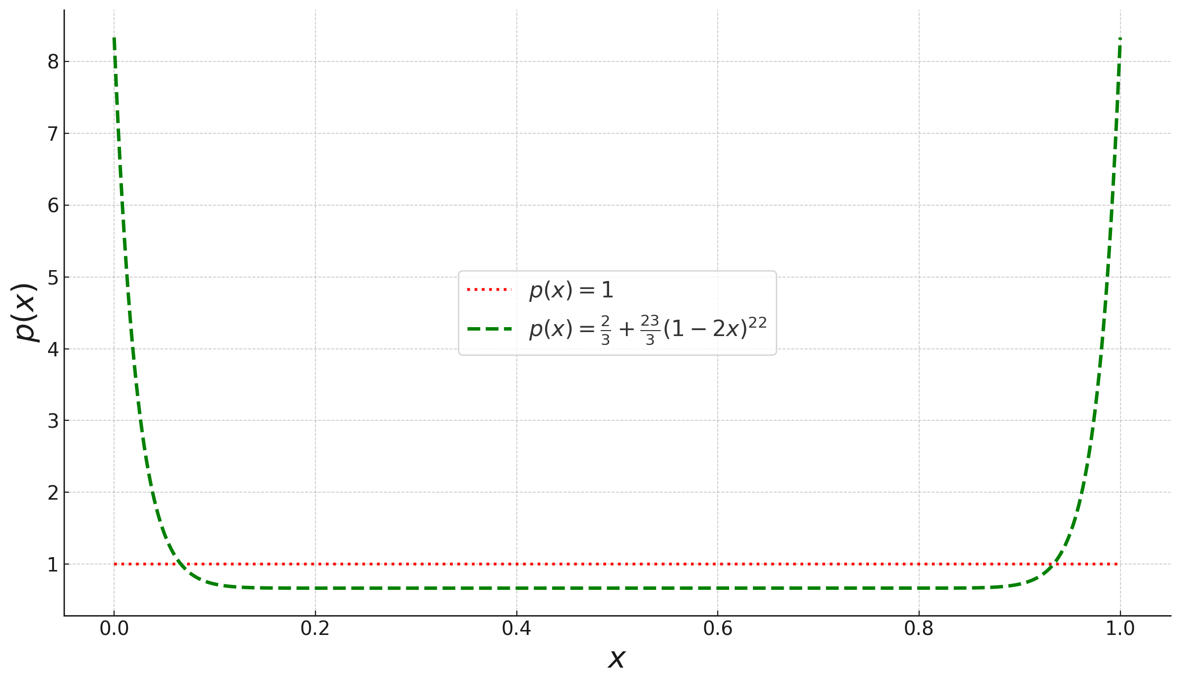
So, in some sense, our goal is to design an independent distribution over labels so that the CDF of is “closer” to . Using numerical verification and exhaustive search, we arrived at the probability distribution over with density . If are sampled independently from , we obtain a CDF for which is closer to in the relevant respect. We show that using this distribution yields a better approximation ratio than uniform labels. Due to the complexity of the resulting expressions, we use numerical verification. Figure 1 shows the comparison of the densities of and .
Theorem 6.
Assigning labels to all vertices from the interval independently according to the density results in an a solution with expected cost below . This results in a randomized -approximation for DED().
Proof.
As in the uniform case, to obtain the theorem it is sufficient to prove the following claim and apply Lemma 3.
Claim 7.
Suppose are independent random variables sampled from , then for all .
Proof.
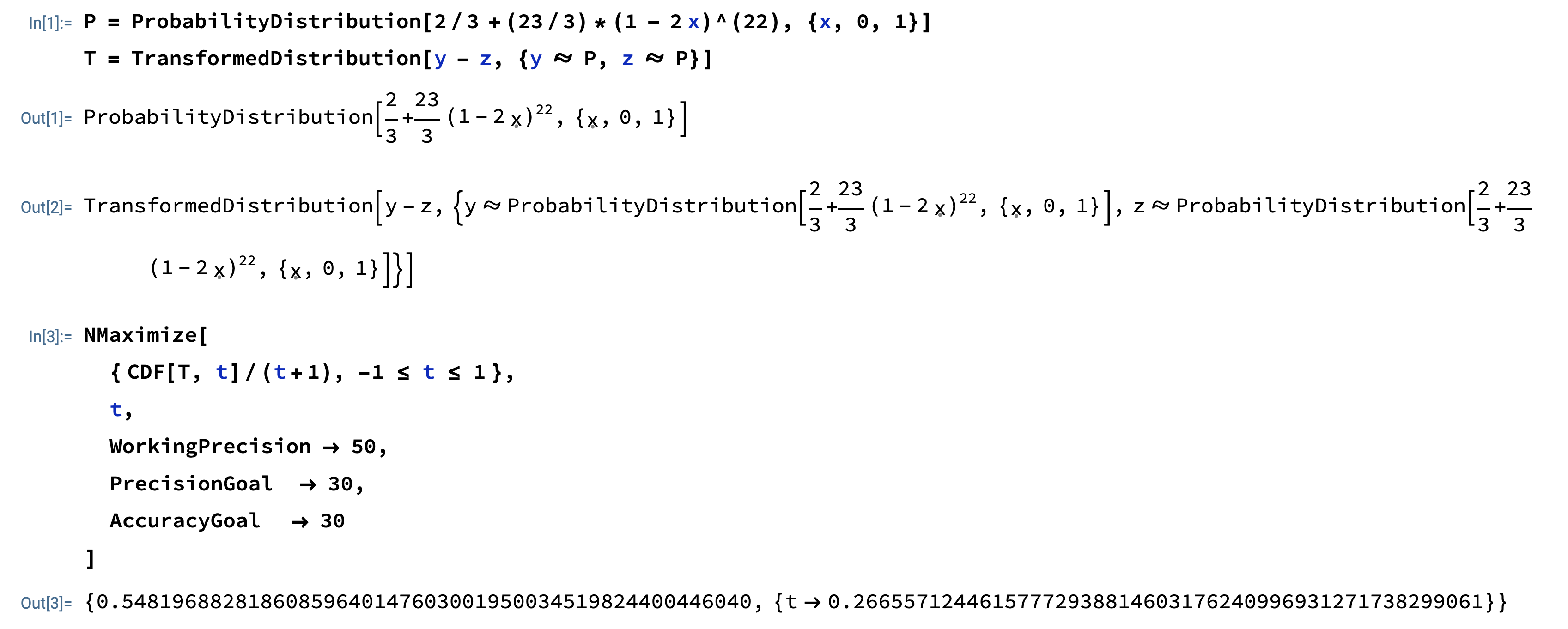
This is verified by Mathematica. See Appendix A for the code used and an execution. The maximum of occurs at approximately with value slightly below . See Figure 3.
3 Lower Bound
An interesting problem is to find the function that minimizes the approximation ratio when using an independent distribution over labels:
Problem 8.
Let denote the set of probability distributions supported on . Find
While this problem does not capture the possibility of correlated label distributions (which we exploit in the bipartite case in Section 4), we find it quite interesting on its own. While some related questions have been studied in additive combinatorics, for example by Cloninger and Steinerberger [5] and Matolcsi and Vinuesa [14], we were unable to find a resolution of this question in the literature. We have been able to bound:
where the upper bound is from Section 2. Here, we show a complete proof of a lower bound of .
Lemma 9.
Proof.
Let be a distribution supported on and be independent samples from . Suppose that
Denote . First note that symmetry of gives the complementary lower bound
These inequalities imply
Fix some that we choose later (so ) and observe that
Integration by parts gives
For (whose CDF is ), we have , therefore
Using and subtracting the two formulas above yields
By symmetry, we have
Since has only one root in , we may use to upper bound the integral
which evaluates to . It follows that
We remark that using the function instead of in the above proof shows a slightly stronger lower bound .
From the Lemma 9 it follows that every distribution has a corresponding CDF of which significantly exceeds the CDF of at some point. Therefore we cannot attain a ratio of . However, this may still be possible for correlated label distributions, and indeed, depending on the structure of the graph such distributions can exist. In the next section we show they can be constructed easily for bipartite graphs.
4 Optimal Rounding for Special Cases
In this section, we show how to obtain our desired bound of for two special cases. The result for bipartite graphs is tight up to constants, while the second result is tight as there is a matching integrality gap on a point with for all edges.
4.1 Bipartite Graphs
Here we show that for any bipartite DAG there exists a distribution over labels so that the randomized algorithm from above achieves an approximation ratio of . Notably, the instances from Kenkre et al. used to obtain UGC hardness of are bipartite, so this is tight up to constants assuming the UGC.
Theorem 10.
Let be bipartite with bipartition and be a feasible solution to (1). Then, there is an algorithm that produces a DED() solution with expected cost at most .
Proof.
Our algorithm is identical to before, except now we produce a correlated distribution over labels. To produce the labeling , we first sample uniformly. Then, with probability , assign for all and for all . Otherwise, assign for all and for all .
For every edge , the distribution over is now uniform over , as with probability we obtain a uniformly random number between and and otherwise a uniformly random number between and . Therefore, if we now run the same algorithm as before, we have:
| As | ||||
as desired. It is unclear whether correlated distributions can be used to improve the approximation ratio in the general case.
4.2 Instances with Structured LP Solutions
Here we show that an independent distribution over labels exists when we have a structured LP solution. It implies, for example, that if our LP solution has the property that for all for some fixed value , we can obtain a -approximation, but is slightly more general (for example, we can obtain the same ratio if all edges have value at least ).
Theorem 11.
If is a feasible solution to (1), and for every edge with we have:
for some integer , then there is an algorithm that produces a solution of expected cost at most . In the case that , the upper bound is not necessary as we may simply cut all edges with value at least and round the remaining edges.
Proof.
Let be the uniform distribution over labels in the set . We claim applying our framework by selecting each label independently from proves the theorem. We cut an edge if
Therefore, since is either negative, 0, or at least , we cut an edge exactly when . So, the probability we cut any edge with is:
Now, the probability we cut an edge compared to (our approximation ratio) is:
As desired.
5 Conclusion
The main open question remaining is whether it is possible to obtain an algorithm with approximation ratio , or whether this is UGC-Hard. We are unaware of any instances with integrality gap above , so improving this bound is also of interest. Another open problem is whether it is NP-Hard to obtain an approximation for DED().
References
- [1] Ron Aharoni, Ron Holzman, and Michael Krivelevich. On a theorem of lovász on covers in -partite hypergraphs. Combinatorica, 16(2):149–174, 1996. doi:10.1007/BF01844843.
- [2] Noga Alon, Béla Bollobás, András Gyárfás, Jenő Lehel, and Alex Scott. Maximum directed cuts in acyclic digraphs. Journal of Graph Theory, 55(1):1–13, 2007. doi:10.1002/jgt.20215.
- [3] Boštjan Brešar, František Kardoš, Ján Katrenič, and Gabriel Semanišin. Minimum -path vertex cover. Discrete Applied Mathematics, 159(12):1189–1195, 2011. doi:10.1016/j.dam.2011.04.008.
- [4] Pierre Charbit, Geoffroy Couteau, Pierre Meyer, and Reza Naserasr. A note on low-communication secure multiparty computation via circuit depth-reduction. In Elette Boyle and Mohammad Mahmoody, editors, Theory of Cryptography, pages 167–199, Cham, 2025. Springer Nature Switzerland.
- [5] Alexander Cloninger and Stefan Steinerberger. On suprema of autoconvolutions with an application to sidon sets. Proceedings of the American Mathematical Society, 145(8):3191–3200, 2017. doi:10.1090/proc/13690.
- [6] Fabrizio Grandoni, Tomasz Kociumaka, and Michał Włodarczyk. An lp-rounding 22-approximation for restricted maximum acyclic subgraph. Information Processing Letters, 115(2):182–185, 2015. doi:10.1016/j.ipl.2014.09.008.
- [7] Venkatesan Guruswami, Rajsekar Manokaran, and Prasad Raghavendra. Beating the random ordering is hard: Inapproximability of maximum acyclic subgraph. In 2008 49th Annual IEEE Symposium on Foundations of Computer Science, pages 573–582, 2008. doi:10.1109/FOCS.2008.51.
- [8] Samuel Safra Irit Dinur. On the hardness of approximating minimum vertex cover. Annals of Mathematics, 162(1):439–485, 2005. URL: http://www.jstor.org/stable/3597377.
- [9] Sreyash Kenkre, Vinayaka Pandit, Manish Purohit, and Rishi Saket. On the approximability of digraph ordering. Algorithmica, 78(4):1182–1205, August 2017. doi:10.1007/s00453-016-0227-7.
- [10] Rohit Khandekar, Tracy Kimbrel, Konstantin Makarychev, and Maxim Sviridenko. On hardness of pricing items for single-minded bidders. In Irit Dinur, Klaus Jansen, Joseph Naor, and José Rolim, editors, Approximation, Randomization, and Combinatorial Optimization. Algorithms and Techniques, pages 202–216, Berlin, Heidelberg, 2009. Springer Berlin Heidelberg. doi:10.1007/978-3-642-03685-9_16.
- [11] Subhash Khot, Dor Minzer, and Muli Safra. On independent sets, 2-to-2 games, and grassmann graphs. In Proceedings of the 49th Annual ACM SIGACT Symposium on Theory of Computing, STOC 2017, pages 576–589, New York, NY, USA, 2017. Association for Computing Machinery. doi:10.1145/3055399.3055432.
- [12] Nathan Klein and Tom Wexler. On the approximability of dag edge deletion, 2015.
- [13] Michael Lampis, Georgia Kaouri, and Valia Mitsou. On the algorithmic effectiveness of digraph decompositions and complexity measures. In Seok-Hee Hong, Hiroshi Nagamochi, and Takuro Fukunaga, editors, Algorithms and Computation, volume 5369 of Lecture Notes in Computer Science, pages 220–231. Springer Berlin Heidelberg, 2008. doi:10.1007/978-3-540-92182-0_22.
- [14] Máté Matolcsi and Carlos Vinuesa. Improved bounds on the supremum of autoconvolutions. Journal of Mathematical Analysis and Applications, 372(2):439–447.e2, 2010. doi:10.1016/j.jmaa.2010.07.030.
- [15] D. Paik, S. Reddy, and S. Sahni. Deleting vertices to bound path length. IEEE Transactions on Computers, 43(9):1091–1096, September 1994. doi:10.1109/12.312117.
- [16] Prasad Raghavendra. Optimal algorithms and inapproximability results for every CSP? In Proceedings of the Fortieth Annual ACM Symposium on Theory of Computing, STOC ’08, pages 245–254, New York, NY, USA, 2008. Association for Computing Machinery. doi:10.1145/1374376.1374414.
- [17] Ola Svensson. Hardness of vertex deletion and project scheduling. In Anupam Gupta, Klaus Jansen, José Rolim, and Rocco Servedio, editors, Approximation, Randomization, and Combinatorial Optimization. Algorithms and Techniques, volume 7408 of Lecture Notes in Computer Science, pages 301–312. Springer Berlin Heidelberg, 2012. doi:10.1007/978-3-642-32512-0_26.
- [18] Jianhua Tu and Wenli Zhou. A factor 2 approximation algorithm for the vertex cover problem. Information Processing Letters, 111(14):683–686, 2011. doi:10.1016/j.ipl.2011.04.009.
- [19] Ryan Williams. Finding paths of length in time. Inf. Process. Lett., 109(6):315–318, February 2009. doi:10.1016/j.ipl.2008.11.004.
Appendix A Automated Verification
Here we include a copy of a high precision run in Mathematica showing a worst case ratio of slightly below 0.5482.
Appendix B Figure 3

