Budget and Profit Approximations for Spanning Tree Interdiction

Ostrovsky, Rafail; Rabani, Yuval; Siman Tov, Yoav

doi:10.4230/LIPIcs.APPROX/RANDOM.2025.7

Budget and Profit Approximations for Spanning Tree Interdiction

Rafail Ostrovsky

University of California, Los Angeles, CA, USA Yuval Rabani The Rachel and Selim Benin School of Computer Science and Engineering, The Hebrew University of Jerusalem, Israel Yoav Siman Tov The Rachel and Selim Benin School of Computer Science and Engineering, The Hebrew University of Jerusalem, Israel

Abstract

We give polynomial time logarithmic approximation guarantees for the budget minimization, as well as for the profit maximization versions of minimum spanning tree interdiction. In this problem, the goal is to remove some edges of an undirected graph with edge weights and edge costs, so as to increase the weight of a minimum spanning tree. In the budget minimization version, the goal is to minimize the total cost of the removed edges, while achieving a desired increase $\Delta$ in the weight of the minimum spanning tree. An alternative objective within the same framework is to maximize the profit of interdiction, namely the increase in the weight of the minimum spanning tree, subject to a budget constraint. There are known polynomial time $O(1)$ approximation guarantees for a similar objective (maximizing the total cost of the tree, rather than the increase). However, the guarantee does not seem to apply to the increase in cost. Moreover, the same techniques do not seem to apply to the budget version.

Our approximation guarantees are motivated by studying the question of minimizing the cost of increasing the minimum spanning tree by any amount. We show that in contrast to the budget and profit problems, this version of interdiction is polynomial time-solvable, and we give an efficient algorithm for solving it. The solution motivates a graph-theoretic relaxation of the NP-hard interdiction problem. The gain in minimum spanning tree weight, as a function of the set of removed edges, is super-modular. Thus, the budget problem is an instance of minimizing a linear function subject to a super-modular covering constraint. We use the graph-theoretic relaxation to design and analyze a batch greedy-based algorithm.

Keywords and phrases:

minimum spanning tree, spanning tree interdiction, combinatorial approximation algorithms, partial cut

Category:

APPROX

Funding:

Rafail Ostrovsky: Distribution Statement “A” (Approved for Public Release, Distribution Unlimited). This material is based upon work supported by the Defense Advanced Research Projects Agency (DARPA) under Contract No. HR001123C0029. Any opinions, findings and conclusions or recommendations expressed in this material are those of the author(s) and do not necessarily reflect the views of the Defense Advanced Research Projects Agency (DARPA).

Yuval Rabani: Research supported in part by ISF grants 3565-21 and 389-22, and by BSF grant 2023607.

Copyright and License:

2012 ACM Subject Classification:

Theory of computation

\rightarrow

Routing and network design problems

DOI:

10.4230/LIPIcs.APPROX/RANDOM.2025.7

Event:

Approximation, Randomization, and Combinatorial Optimization. Algorithms and Techniques (APPROX/RANDOM 2025)

Editors:

Alina Ene and Eshan Chattopadhyay

Series and Publisher:

Leibniz International Proceedings in Informatics, Schloss Dagstuhl – Leibniz-Zentrum für Informatik

1 Introduction

Problem statement and results

This paper deals with spanning tree interdiction. The basic setting is an undirected finite graph with edge weights and edge costs. By removing some edges, the weight of a minimum spanning tree can be increased, at a cost equal to the sum of costs of the removed edges. This setting gives rise to various optimization formulations. We consider primarily the following case, which we call the budget problem: we are given a target $\Delta$ by which to increase the weight of a minimum spanning tree, and the optimization objective is to minimize the cost of doing so. In the alternative profit problem, we are given a budget $B$ , and the optimization objective is to maximize the damage, namely the increase in the weight of a minimum spanning tree, subject to the cost not exceeding $B$ .

Both problems are NP-hard (see [17]). Our main result is a polynomial time $O(\log n)$ approximation algorithm for the budget problem. The approximation algorithm is motivated by considering the following special case: minimize the cost of increasing the weight of a minimum spanning tree, by any amount. We show that in contrast with the general budget problem, this objective can be optimized in polynomial time, and we give an efficient algorithm for computing the optimum. We also give $O(\log n)$ -approximation guarantees for the profit problem. Finally, we investigate the question of defending against interdiction by adding edges to the input graph. The set of edges to choose from is given, and each edge is endowed with a cost of constructing it.

Motivation

The primary application of interdiction computations is to examine the sensitivity of combinatorial optimization solutions to partial destruction of the underlying structure. This can be used either to detect vulnerabilities in desirable structures, or to utilize vulnerabilities to impair undesirable structures. The budget problem is perhaps more suitable in the former setting, as its solution indicates the cost of inflicting a (dangerous) level of damage. The profit problem is perhaps more suitable in the latter setting, as it aims to maximize the damage inflicted using limited resources. Such problems arise in a variety of application areas, including military planning, infrastructure protection, law enforcement, epidemiology, etc. (see, for example the references in [24]).

Related work

Previous work on spanning tree interdiction focuses exclusively on a version of the profit problem. It approximates the total weight of the post-interdiction minimum spanning tree, rather than the increase $\Delta$ in the weight of the tree as per the above definition of the profit problem. Notice that if the resulting tree has total weight which is $C$ times the weight of the initial tree, then approximating the total weight by any factor at least $C$ means the algorithm could end up doing nothing. In contrast, approximation of the profit problem guarantees actual interdiction even if $\Delta$ is very small compared with the weight of the initial tree. Note that in the case of the budget problem there is no qualitative difference between specifying the target total weight and specifying the target increase in weight.

The case of uniform cost was first considered in [8] who gave a poly-time $O(\log B)$ approximation algorithm for the (total tree weight version of the) profit problem, where $B$ is the budget (i.e., the number of edges the algorithm is allowed to remove). They showed that the uniform cost problem is NP-hard (previously, it was known that the problem with arbitrary costs is NP-hard; see [17] and the references in [8]). The same problem was also discussed in [4] and the references therein, where algorithms running in time that is exponential in the budget $B$ were considered. Later, constant factor approximation algorithms for the problem, without the cost-uniformity constraint, were found [24, 16]. The latter paper gave a $4$ -approximation guarantee. The upper bound that was used in both papers cannot be used to get an approximation better than $3$ [16]. In [11] it was shown that the problem is fixed parameter-tractable (parametrized by the budget $B$ ), but the budget problem is $W[1]$ -hard (parametrized by the weight of the resulting tree).

We briefly review the constant factor approximation guarantees for total minimum spanning tree weight in [24, 16]. Both papers use the following framework. ( $i$ ) Let $w_{1}\leq w_{2}\leq\cdots\leq w_{k}$ be the sorted list of distinct edge weights, and let $G_{1},G_{2},\dots,G_{k}$ denote the subgraphs of the input graph $G$ , where the edges of $G_{i}$ are all the edges of $G$ of weight at most $w_{i}$ . Then, the objective function at a set $F$ of removed edges can be expressed as a function of the number of connected components of $G_{i}\setminus F$ and $w_{i}-w_{i-1}$ , for all $i$ . This implies, in particular, that the objective function is super-modular. ( $i i$ ) Maximizing an unconstrained super-modular function is a polynomial time-computable problem. Hence, the Lagrangian relaxation of the linear budget constraint can be computed efficiently for any fixed setting of the Lagrange multiplier. Binary search can be used to find a good multiplier. The usual impediment of this approach shows up here as well. The search resolves the problem only if the solution spends exactly the upper bound on the cost. However, it may end up producing two solutions for (essentially) the same Lagrange multiplier, one below budget and one above budget. Those combine to form a bi-point fractional solution. ( $i i i$ ) How to extract a good integral solution from this bi-point solution is where the papers diverge. The tighter approximation of [16] reduces, approximately, the problem of extracting a good solution to the problem of tree knapsack, then uses a greedy method to approximate the latter problem. The former result of [24] used a more complicated argument, but also a greedy approach. We give an example (in Section 6) that these algorithms do not perform well in terms of approximating the increase $\Delta$ in spanning tree weight.

Super-modularity carries over to the objective function we use here, namely the increase in the weight of a minimum spanning tree, as the difference between the functions is a constant (the weight of the spanning tree before interdiction). Thus, as the above discussion hints to, the profit problem is a special case of the problem of maximizing a monotonically non-decreasing and non-negative super-modular function subject to a linear packing constraint (a.k.a. a knapsack constraint). Similarly, the budget problem is a special case of minimizing a non-negative linear function subject to a super-modular covering constraint (i.e., a lower bound on a non-decreasing and non-negative super-modular function).

Similar settings are prevalent in combinatorial optimization. A generic problem of this flavor is set cover, which is a special case of minimizing a non-negative linear function subject to a monotonically non-decreasing and non-negative sub-modular covering constraint. The related maximum coverage problem is a special case of maximizing a monotonically non-decreasing and non-negative sub-modular function, subject to a cardinality constraint (which is, of course, a special case of a knapsack constraint). More broadly, many problems that arise in unsupervised machine learning are of this flavor. For example, $k$ -means and $k$ -median clustering are special cases of minimizing a monotonically non-increasing and non-negative sub-modular function subject to a cardinality constraint. Several such formulations received general treatment; see for example [18, 20, 7, 22, 13, 19, 15, 1] and the references therein. Obviously, an optimization problem has equivalent representations derived by transformations between super-modularity and sub-modularity, maximization and minimization, and/or covering and packing (by defining the function over the complement set, or negating). These transformations reverse monotonicity, and moreover may not preserve approximation bounds.

The particular combination of super-modular maximization subject to a knapsack constraint is known as the super-modular knapsack problem, introduced in [9]. In general, it is hard to approximate within any factor (given query access to a monotonically non-decreasing objective function subject to a cardinality constraint); see the example in [21]. The case of a symmetric (therefore, non-monotone) super-modular function can be solved exactly in polynomial time [10]. We are not aware of any relevant work on the problem of approximating the minimum of a non-negative linear objective, subject to a super-modular covering constraint. The convex hull of the indicator vectors that satisfy a generic super-modular covering constraint is investigated in [2].

Finally, we mention that spanning tree interdiction is one problem in a large repertoire of interdiction problems, including in particular interdiction of shortest path, assignment and matching problems, network flow problems, linear programs, etc. Some representative papers include [14, 23, 3, 5, 6, 12] (this list is far from being comprehensive).

Our techniques

Our results rely on the notion of a partial cut, which is the set of edges that cross a cut with weight below a given threshold weight. An optimal solution minimizing the cost of increasing the weight of a minimum spanning tree by any amount is a single partial cut. We show that such a cut can be computed efficiently by enumerating over a polynomial time computable collection of candidate partial cuts. In order to derive the approximation guarantees for the general budget problem, we apply a batch greedy approach. We repeatedly compute the collection of candidate partial cuts and choose a cut with the best gain per cost ratio. The proof of approximation guarantee relies on an approximate characterization of an optimal solution by a collection of partial cuts. We further show how to speed up the computation by using in all iterations the collection computed for the input graph, rather than recomputing a new collection in each iteration. A similar approach gives the logarithmic approximation for the profit problem, in a manner parallel to the greedy approximation for knapsack (i.e. use either the maximum greedy solution that does not exceed the budget, or the best single partial cut).

Organization

In Section 2 we present some useful definitions and claims, including a self-contained (and different) proof of super-modularity of the gain in spanning tree weight function. In Section 3 we give a polynomial time algorithm for minimizing the cost of increasing the minimum spanning tree weight by any amount. This algorithm motivates our approximation algorithm for the budget problem. In Section 4 we present our graph-theoretic relaxation. In Section 5 we present our main result – an approximation algorithm for the budget problem. In Section 6 we give an approximation algorithm for the profit problem, and discuss the shortcoming of previous work to achieve this objective. Finally, in Section 7 we remark on defense against spanning tree interdiction.

2 Preliminaries

In this section we present some general definitions and useful lemmas.

Let $G=(V,E)$ be a weighted undirected graph such that every edge $e$ has a non-negative weight $w:E\rightarrow\mathbb{R}^{+}\cup\{0\}$ and a positive removal cost $c:E\rightarrow\mathbb{R}^{+}$ . Let $\operatorname{MST}(G)$ denote the weight of a minimum spanning tree of $G$ . We’ll use the convention that if $G$ is disconnected, then $\operatorname{MST}(G)=\infty$ . Also, for a set of edges $F\subset E$ , we denote $c(F)=\sum_{f\in F}c(f)$ . Given a budget $B$ , the spanning tree Interdiction problem is to find a set of edges $F\subset E$ satisfying $c(F)\leq B$ and maximizing $\operatorname{MST}(G\setminus F)$ , where $G\setminus F$ denotes the graph $(V,E\setminus F)$ . The profit $p_{G}(F)$ of a solution $F$ to the spanning tree interdiction problem is defined to be the increase $p_{G}(F)=\operatorname{MST}(G\setminus F)-\operatorname{MST}(G)$ in the weight of the minimum spanning tree. The profit to cost ratio of a set of edges $F\subset E$ is defined to be $r_{G}(F)=\frac{p_{G}(F)}{c(F)}$ . For the empty set ( $c(F)=0$ ), we define $r_{G}(\emptyset)=0$ .

Consider a weighted graph $G=(V,E)$ as above. Given a set of nodes $S$ , $\emptyset\neq S\subsetneq V$ , The complete cut $C=C_{G}(S)$ defined by $S$ is the set of edges

C=C_{G}(S)=\{e\in E:\ |e\cap S|=1\}.

We say that the edges in $C$ cross the cut $C=C_{G}(S)$ . Given $S$ and $W\in\mathbb{R}^{+}$ , the partial cut $C=C_{G}(S,W)$ is the set of edges

C=C_{G}(S,W)=\{e\in C_{G}(S):\ w(e)<W\}.

Consider a connected graph $G$ , let $T$ be a spanning tree of $G$ , and let $e\in T$ . We denote by $C_{T,e}$ the cut in $G$ that satisfies $C_{T,e}\cap T=e$ .
We show the following lemmas that will be useful later (the proofs are in Appendix A).

Lemma 1.

Consider a minimum spanning tree $T$ of a connected graph $G$ . Let $F\subset E$ such that $G^{\prime}=G\setminus F$ is connected. Then, there exists a minimum spanning tree $T^{\prime}$ for $G^{\prime}$ that includes all the edges in $T\setminus F$ .

Lemma 2.

Let $G=(V,E)$ be a $w$ -weighted graph and let $C=C_{G}(S,W)\subseteq E$ be a partial cut in $G$ . Let $e=(u,v)\in E$ be an edge that crosses $C_{G}(S)$ . Then,

p_{G}(C)\geq W-w(e).

The following lemma reproves a claim from [24].

Lemma 3 (super-modularity of the profit function).

Let graph $G=(V,E)$ be a $w$ -weighted graph, let $B\subset E$ be set of edges, and let $e\in E\setminus B$ be an edge. If $G\setminus B$ is connected, then

p_{G\setminus B}(e)\geq p_{G}(e).

Corollary 4.

Let $G=(V,E)$ be a weighted graph, and let $A,B\subset E$ be disjoint sets of edges ( $A\cap B=\emptyset$ ). Then

p_{G\setminus B}(A)\geq p_{G}(A).

3 An Algorithm for $\varepsilon$ -Increase

In this section we design and analyze a polynomial time algorithm for computing the minimum cost interdiction to increase the weight of a minimum spanning tree (by any amount). I.e., given a graph $G=(V,E)$ with edge weights $w$ and edge costs $c$ , we want to find a set of edges $F\subset E$ for which $\operatorname{MST}(G\setminus F)>\operatorname{MST}(G)$ , minimizing $c(F)$ . This algorithm motivates our approximation algorithm for the budget problem given in Section 5 (and its derivative for the profit problem in Section 6).

The algorithm is defined as follows. Compute a minimum spanning tree $T$ of $G$ . Enumerate over all the edges $e\in T$ . Given an edge $e$ , contract all the edges of weight $<w(e)$ . Remove all edges of length $>w(e)$ . Find a minimum (with respect to edge cost) $u$ - $v$ cut in the resulting graph, where $e=\{u,v\}$ . The output of the algorithm $F_{\min}$ is the minimum cost cut generated, among all choices of $e\in T$ .

The following two claims imply that the output of the algorithm is valid and optimal (the proofs are in Appendix A).

Claim 5.

$c(F_{\min})\leq c(F^{*})$ , where $F^{*}$ is an optimal solution.

Claim 6.

$\operatorname{MST}(G\setminus F_{\min})>\operatorname{MST}(G)$ .

Let $\tau(n,m)$ denote the time to compute a minimum $s$ - $t$ cut in a graph with $n$ nodes and $m$ edges.

Corollary 7.

The algorithm finds an optimal solution in time $O(n\cdot\tau(|V|,|E|))$ .

Proof.

Recall that $F_{\min}$ is the solution that the algorithm computes. By Claim 5, $c(F_{\min})\leq c(F^{*})$ , and by Claim 6 we have $\operatorname{MST}(G\setminus F_{\min})>\operatorname{MST}(G)$ , so $F_{\min}$ is an optimal solution. The algorithm iterates over the $|V|-1$ edges of $T$ , and for each edge calculates a minimum cut, hence the time complexity. $\hfill\blacktriangleleft$

4 Relaxed Specification of the Optimum

In this section, we define a relaxation to the optimal solution for the budget minimization problem, based on a carefully constructed collection of partial cuts. We will then use this relaxation to analyze our approximation algorithms.

Given a solution $F$ with cost $B=c(F)$ and profit $\Delta$ , we construct a sequence of cuts $C_{1},C_{2},\ldots,C_{t-1}$ that satisfy the following properties regarding their cost and profit.

Theorem 8.

Let $G=(V,E)$ be an undirected graph, and let $n=|V|$ . Also, let $F\subseteq E$ be a set of edges of cost $B=c(F)$ and profit $\Delta$ . Then, there exists a sequence of partial cuts $C_{1},C_{2},\ldots,C_{t-1}$ such that

\sum_{i=1}^{t-1}c(C_{i})\leq 2B\cdot\log n,\qquad\text{and}\qquad\sum_{i=1}^{t% -1}p_{G}(C_{i})\geq\Delta.

Constructing the sequence of the cuts

Let $G=(V,E)$ be a graph, and let $T$ be a minimum spanning tree in $G$ . Let $F\subset E$ be a set of edges with cost $B$ and profit $\Delta$ . Denote $G\setminus F$ by $G^{\prime}$ . The solution $F$ removes some edges of $G$ , including $t-1$ edges $e_{1},e_{2},\ldots,e_{t-1}$ of $T$ . Notice that $t\leq n-1$ , and if all removal costs are $1$ , also $t\leq B$ . Removing those edges splits $T$ into $t$ connected components $A_{1},A_{2},\ldots,A_{t}$ . We emphasize that $A_{i}$ denotes the node set of the $i$ -th connected component. Therefore, this is a partition of the nodes of $G$ . Let $T^{\prime}$ be a minimum spanning tree of $G^{\prime}$ . By Lemma 1, we can choose $T^{\prime}$ which uses the same edges as $T$ inside the connected components $A_{1},A_{2},\ldots,A_{t}$ , and reconnects these components using $t-1$ new edges to replace the removed edges $e_{1},e_{2},\ldots,e_{t-1}$ .

In the following construction we consider the connected components graph $G_{cc}^{\prime}=(V_{cc},E_{cc}^{\prime})$ , where $V_{cc}=\{A_{1},A_{2},\ldots,A_{t}\}$ , and $E_{cc}^{\prime}$ includes an edge between $A_{i}$ and $A_{j}$ for every pair of vertices $u\in A_{i}$ and $v\in A_{j}$ such that $\{u,v\}\in E^{\prime}$ (with the same weight as the corresponding edge in $G^{\prime}$ ). Notice that $G_{cc}^{\prime}$ may have many parallel edges, and every edge of $G_{cc}^{\prime}$ corresponds to an edge of $G^{\prime}$ . To avoid notational clutter, we will use the same notation for an edge of $G_{cc}^{\prime}$ and for the corresponding edge of $G^{\prime}$ . Also, we will use the same notation for a vertex of $G_{cc}^{\prime}$ and for the corresponding set of vertices of $G^{\prime}$ (which is the same as the vertices of $G$ ), as well as for a set of vertices of $G_{cc}^{\prime}$ and for the union of the corresponding sets of vertices of $G^{\prime}$ . The interpretation will be clear from the context. The idea behind defining $G_{cc}^{\prime}$ is to hide the edges that $T$ and $T^{\prime}$ share inside the connected components, so that the cuts we construct can’t delete them. We use $G_{cc}^{\prime}$ only in order to construct the sequence of cuts (these are cuts in $G$ ). Let $T_{cc}^{\prime}$ be a minimum spanning tree of $G_{cc}^{\prime}$ . Note that $T_{cc}^{\prime}$ has $t-1$ edges, which we denote by $e_{1}^{\prime},e_{2}^{\prime},\ldots,e_{t-1}^{\prime}$ . These edges correspond exactly to the new edges of a minimum spanning tree $T^{\prime}$ of $G^{\prime}$ that replace the edges $e_{1},e_{2},\ldots,e_{t-1}\in T\cap F$ . For the construction, a strict total order on the weights of the edges of $T_{cc}^{\prime}$ is needed. We index these edges in non-decreasing order, breaking ties arbitrarily.

Two alternatives

For each edge $e_{i}^{\prime}$ , we first define two alternatives for a partial cut, $C_{i}^{R}$ or $C_{i}^{L}$ , and later we choose only one of them. This choice is repeated for every edge in $T_{cc}^{\prime}$ to get the desired collection of $t-1$ cuts. Consider $e_{i}^{\prime}$ to be an edge in $T_{cc}^{\prime}$ of weight $w(e_{i}^{\prime})$ . Delete from $T_{cc}^{\prime}$ all the edges $e_{j}^{\prime}$ , $j\geq i$ . Consider the connected components of the resulting forest. Notice that the edge $e_{i}^{\prime}$ must connect between two such components $L_{i}$ and $R_{i}$ (recall that these denote both sets of vertices of $G_{cc}^{\prime}$ and the corresponding unions of sets of vertices of $G$ ). Define the following two partial cuts: $C_{i}^{L}=C_{G}(L_{i},w(e_{i}^{\prime}))$ and $C_{i}^{R}=C_{G}(R_{i},w(e_{i}^{\prime}))$ . We will denote by $X_{i}$ the choice we make between $L_{i}$ and $R_{i}$ , which we refer to as the small side of the cut in step $i$ . Also, we put $C_{i}=C_{G}(X_{i},w(e_{i}^{\prime}))$ , the cut chosen in step $i$ .

Refer to caption — Figure 1: The two options of some edge $e_{i}^{\prime}$ over the MST of the connected components graph.

Choosing $X_{i}$

The goal is that any $A_{j}\in V_{cc}$ will not be contained in “too many” $X_{i}$ -s. We count for each vertex $A_{j}\in V_{cc}$ how many times it was chosen to be in the small side. Denote this number as $k(A_{j})$ , and for a set of vertices $S\subseteq V_{cc}$ denote $k(S)=max_{A_{j}\in S}(k(A_{j}))$ .

We choose cuts in ascending order of $i$ . If $k(L_{i})\leq k(R_{i})$ , we choose $X_{i}=L_{i}$ , and otherwise we choose $X_{i}=R_{i}$ . After choosing a new $X_{i}$ , we increase by $1$ the counter $k(A_{j})$ for every vertex $A_{j}\in X_{i}$ , then proceed to choosing the next cut.

The following lemma shows that the $X_{i}-s$ form a laminar set system over the vertices.

Lemma 9.

Let $i>j$ . Then, either $X_{i}\cap X_{j}=\emptyset$ , or $X_{i}\supset X_{j}$ .

Proof.

Assume that $X_{j}\cap X_{i}\neq\emptyset$ . Let $A\in X_{j}\cap X_{i}$ be a common vertex. Consider a vertex $A^{\prime}\in X_{j}$ . Clearly, there exists a path $P$ connecting $A$ and $A^{\prime}$ in the tree $T_{cc}^{\prime}$ , such that every edge in this path precedes $e_{j}^{\prime}$ in the non-decreasing order; otherwise, $A$ and $A^{\prime}$ would not be in the same connected component of the tree $T_{cc}^{\prime}$ after deleting all the edges preceding $e_{j}^{\prime}$ . Because $e_{i}^{\prime}$ comes after $e_{j}^{\prime}$ , it also holds that both $A$ and $A^{\prime}$ are in the same component of the tree $T_{cc}^{\prime}$ after deleting all the edges with index at least $i$ . This implies that if $A\in X_{i}$ , then also $A^{\prime}\in X_{i}$ , and therefore $X_{j}\subset X_{i}$ . $\hfill\blacktriangleleft$

We now show that the first claim of Theorem 8 holds.

Lemma 10.

The sum of the costs of the cuts $C_{1},C_{2},\ldots,C_{t-1}$ is

\sum_{i=1}^{t-1}c(C_{i})\leq 2B\cdot\log t\leq 2B\cdot\log n.

The proof of Lemma 10 relies on the following claims.

Claim 11.

For every $i=1,2,\dots,t$ , if $e\in C_{i}$ then $e\in F$ .

Proof.

Let’s assume for contradiction that there exists an edge $e\in C_{i}$ , but $e\notin F$ . By construction, $w(e)<w(e_{i}^{\prime})$ . Recall that $C_{i}$ is the set of edges with exactly one endpoint in a connected component $X_{i}$ of $T_{cc}^{\prime}$ after removing edges of weight $\geq w(e_{i}^{\prime})$ . In particular, $e=\{u,v\}$ , where $u\in A_{i}\in X_{i}$ and $v\in A_{j}\not\in X_{i}$ . Consider the path in $T_{cc}^{\prime}$ between $A_{i}$ and $A_{j}$ . There must be an edge $e^{\prime}$ of weight $w(e^{\prime})\geq w(e_{i}^{\prime})$ along this path, otherwise both $u$ and $v$ would be on the same side of the cut. We assumed that $e\not\in F$ , hence $e\in E_{cc}^{\prime}$ . But if $w(e)<w(e_{i}^{\prime})\leq w(e^{\prime})$ and $e\in E_{cc}^{\prime}$ , then replacing $e^{\prime}$ with $e$ in $T_{cc}^{\prime}$ creates a spanning tree of $G_{cc}^{\prime}$ which is lighter than $T_{cc}^{\prime}$ , a contradiction. $\hfill\vartriangleleft$

Next we show that no edge gets deleted by more than $2\cdot\log t$ cuts.

Claim 12.

For any edge $e\in E$ , $e$ crosses no more than $2\cdot\log t$ cuts $C_{1},C_{2},\dots,C_{t-1}$ .

Proof.

Let $\{A_{1},A_{2},\ldots A_{t}\}$ be the vertex set of the graph $G_{cc}^{\prime}$ , and consider the final counts $k(A_{1})$ , $k(A_{2})$ , $\ldots$ , $k(A_{t})$ for the vertices, respectively, after the construction of the cuts $C_{1},C_{2},\ldots C_{t-1}$ as described above. We show that for every $1\leq i\leq t$ , it holds that $k(A_{i})\leq\log(t)$ . This means that every vertex can’t be in the small side of a cut more than $\log(t)$ times, and therefore an edge can’t cross more than $2\cdot\log(t)$ cuts.

We first show that for every $A\in L_{i}\cup R_{i}$ it holds that at the end of step $i$ , $k(A)\leq\log(|L_{i}|+|R_{i}|)$ (viewing $L_{i},R_{i}$ as sets of vertices in $G_{cc}^{\prime}$ ). The proof is by induction on $i$ .

Base case: Notice that $|L_{1}|,|R_{1}|\geq 1$ . Therefore, $\log(|L_{i}|+|R_{i}|)=1$ . As only one step was executed, for every vertex $A$ , we have that $k(A)\leq 1$ , as required.

Inductive step: Assume the claim is true for every $j<i$ . Let $s=|R_{i}|+|L_{i}|$ . It must hold that either $|L_{i}|\leq\frac{s}{2}$ or $|R_{i}|\leq\frac{s}{2}$ . Assume without loss of generality that $|R_{i}|\leq\frac{s}{2}$ . Consider the largest value of $k(A)$ for any $A\in R_{i}$ at the end of step $i-1$ . For this $A$ , let $X_{j}$ be a small side that contains $A$ , for the largest such $j<i$ . As $w(e_{j}^{\prime})\leq w(e_{i}^{\prime})$ , it must be that $R_{j},L_{j}\subset R_{i}$ . This is true because the edges of weight below $w(e_{i}^{\prime})$ include the edges of weight at most $w(e_{j}^{\prime})$ , so $R_{j},L_{j}$ are in the same component $R_{i}$ (as $A\in R_{i}\cap X_{j}$ ). Because $R_{j}\cap L_{j}=\emptyset$ it holds that $|R_{j}|+|L_{j}|\leq|R_{i}|\leq\frac{s}{2}$ . By the induction hypothesis, at the end of step $j$ , we have that $k(A)\leq\log(\frac{s}{2})=\log(s)-1$ . Therefore, this is true also at the end of step $i-1$ , because $k(A)$ did not change after step $j$ and before step $i$ . If $X_{i}=R_{i}$ , then after step $i$ , we get that $k(A)$ increases by $1$ to $\log(s)$ , as claimed. If $X_{i}=L_{i}$ , then $k(A)$ does not change in step $i$ , so it holds that $k(A)\leq\log(s)-1<\log(s)$ .

Finally, consider $A^{\prime}\in L_{i}$ . By the same argument as for $R_{i}$ , at the end of step $i-1$ we have that $k(A^{\prime})\leq\log(|L_{i}|)\leq\log(s-1)<\log(s)$ . If $X_{i}\neq L_{i}$ , then this holds after step $i$ . Otherwise, by the choice of $X_{i}$ it must hold that before step $i$ , $k(A^{\prime})\leq k(A)\leq\log(s)-1$ . Therefore, after step $i$ , $k(A^{\prime})\leq\log(s)$ . $\hfill\vartriangleleft$

Proof of Lemma 10.

By Claim 11, any edge included in at least one of the partial cuts is included in $F$ .

By Claim 12, no edge crosses more than $2\cdot\log(t)$ partial cuts. Because the cuts use only edges from $F$ and use each edge up to $2\cdot\log(t)$ times, the sum of their costs is no more than $2B\cdot\log(t)\leq 2B\cdot\log n$ . $\hfill\blacktriangleleft$

It remains to show the second claim of Theorem 8.

Lemma 13.

For the cuts $C_{1},C_{2},\ldots,C_{t-1}$ it holds that $\sum_{i=1}^{t-1}p_{G}(C_{i})\geq\Delta$

The first step of the proof is to show a perfect matching between the edges that were removed from $T$ (a minimum spanning tree of $G$ ) and the new edges that replaced them in $T^{\prime}$ (a minimum spanning tree of $G\setminus F$ ). We will use this matching to argue that for every matched pair there is a cut with a profit of at least the difference of weights between the edges, and this will be used to lower bound the total profit. To show the existence of a perfect matching, we employ Hall’s condition. We begin with the following claim.

Claim 14.

Let $C_{1},C_{2},\ldots,C_{t-1}$ be the cuts induced by $T$ and $F$ . Then, for every cut $C_{i}$ there exists a vertex $v_{i}\in V_{cc}$ such that $v_{i}\in X_{i}$ , but $v_{i}\notin X_{j}$ for all $j<i$ . Moreover, there exists a vertex $u\in V_{cc}$ such that $u\notin X_{j}$ for all $j\in[t-1]$ .

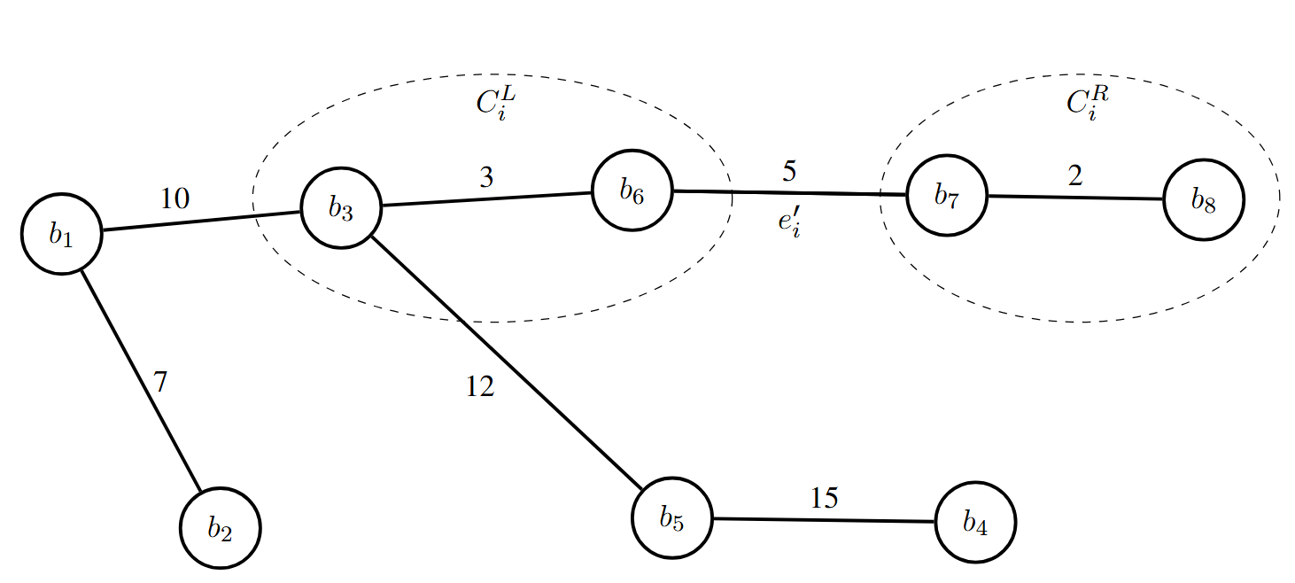
We refer to $v_{i}$ as the typical vertex of $C_{i}$ , and to $u$ as the typical vertex of the graph; see Figure 2; $b_{6}$ is the typical vertex of the cut with the weight of $w=10$ , and $b_{2}$ is the typical vertex of the graph.

Proof of Claim 14.

Consider $X_{i}$ . Every edge $e\in T_{cc}^{\prime}$ with both endpoints in $X_{i}$ has index $<i$ and every edge $e\in T_{cc}^{\prime}$ that connects between $X_{i}$ and $V_{cc}\setminus X_{i}$ must have index $\geq i$ . Clearly, if $X_{j}\cap X_{i}=\emptyset$ , then any choice of $v_{i}\in X_{i}$ will satisfy $v_{i}\not\in X_{j}$ . By Lemma 9, all other $j<i$ satisfy $X_{j}\subsetneq X_{i}$ .

It is sufficient to consider all $j$ such that $X_{j}\subsetneq X_{i}$ and $\not\exists j^{\prime}$ such that $X_{j}\subsetneq X_{j^{\prime}}\subsetneq X_{i}$ . Let $j_{1}<j_{2}<\cdots<j_{l}$ be an enumeration of these indices. Notice that $|X_{j_{1}}\cap e_{j_{1}}^{\prime}|=1$ . Moreover, for $r>1$ , $X_{j_{r}}\cap e_{j_{1}}^{\prime}=\emptyset$ . This is because $e_{j_{1}}^{\prime}$ and all the edges with two endpoints in $X_{j_{1}}$ are not deleted when constructing $X_{j_{r}}$ . Therefore, if $X_{j_{r}}\cap e_{j_{1}}^{\prime}\neq\emptyset$ , then $X_{j_{r}}\supset X_{j_{1}}$ , in contradiction to the definition of $j_{1}$ . However, $X_{i}\supset X_{j_{r}}$ for all $r$ , and $e_{j_{1}}^{\prime}$ is not deleted when constructing $X_{i}$ , hence both endpoints of $e_{j_{1}}^{\prime}$ are contained in $X_{i}$ . The endpoint not contained in $X_{j_{1}}$ can be used as the typical vertex $v_{i}$ of $C_{i}$ .

The same argument, applied with $V_{cc}$ replacing $X_{i}$ , proves the existence of the typical vertex $u$ of $G$ . $\hfill\vartriangleleft$

Next we prove the following claim.

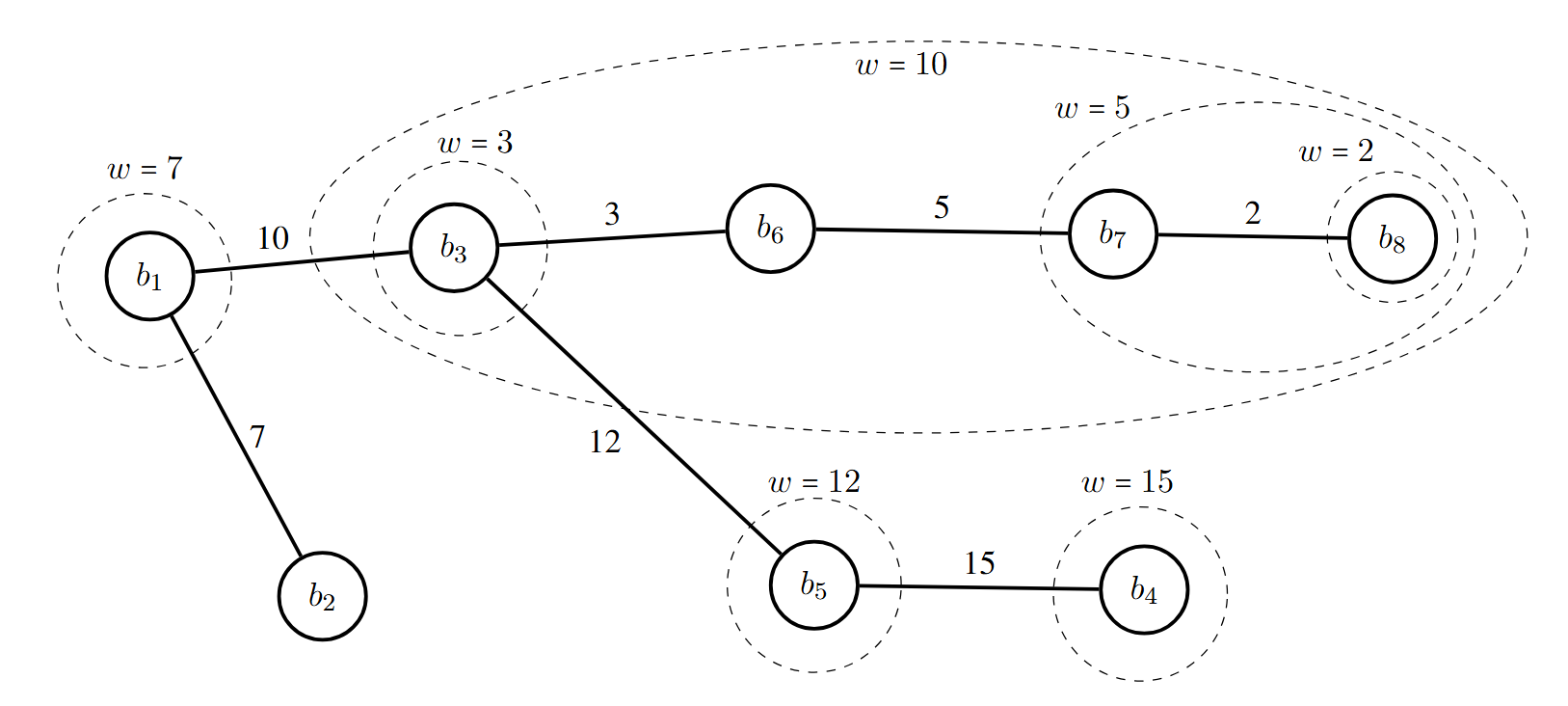
Claim 15.

For every $k\in\{1,2,\dots,t-1\}$ and for every $A\subseteq\{C_{1},C_{2},\ldots,C_{t-1}\}$ of cardinality $|A|=k$ , there exist at least $k$ distinct edges $e_{1},\ldots e_{k}\in F\cap T$ that cross at least one of the cuts in $A$ .

Proof.

The edges in $F\cap T$ by definition form a spanning tree on $V_{cc}$ equipped with the edges of the original graph $G$ .

Given a set $A$ of $k$ cuts, we say that two vertices $A_{i},A_{j}\in V_{cc}$ are in the same area if and only if they are in the same side of any cut in $A$ . Notice that the partition into areas is an equivalence relation as it is reflexive, symmetric and transitive. We claim that there are at least $k+1$ different areas, because there are at least $k+1$ vertices for which every pair of them is not in the same area (separated with at least one cut). Each of the cuts in $A$ has a typical vertex. Any pair of two typical vertices $v_{i},v_{j}$ , $i\neq j$ cannot be in the same area. If the two cuts are disjoint ( $X_{i}\cap X_{j}=\emptyset$ ) then $v_{i}\in X_{i}$ but $v_{j}\not\in X_{i}$ . Otherwise, one contains the other ( $X_{i}\subset X_{j}$ ), but $v_{i}\in X_{i}$ whereas $v_{j}\in X_{j}\setminus X_{i}$ . Moreover, the typical vertex of the graph is not in the same area as any of the other typical vertices (because it not in any $X_{i}$ ). To cap, in total there are at least $k+1$ areas, and any edge between two different areas must cross at least one cut in $A$ . The spanning tree $F\cap T$ has to connect, in particular, all the vertices in the different areas, so it must have at least $k$ edges that connect vertices in two different areas. $\hfill\vartriangleleft$

Claim 16.

There exists a permutation $\pi$ on $\{1,2,\dots,t-1\}$ such that $e_{\pi(i)}\in C_{i}$ and

\sum_{i=1}^{t-1}\left(w(e_{i}^{\prime})-w(e_{\pi(i)})\right)=\Delta.

Proof.

By Claim 15 and Hall’s marriage theorem we conclude that there exists a perfect matching between the $t-1$ cuts and the $t-1$ edges of $T\cap F$ , where an edge and a cut are matched only if the edge crosses the cut. Every cut $C_{i}$ is constructed using the edge $e_{i}^{\prime}$ and a weight of $w(e_{i}^{\prime})$ . Let $e_{\pi(i)}$ be the edge matched to $C_{i}$ , so $e_{\pi(i)}$ crosses $C_{i}$ .

Let $\{e_{1},e_{2},\ldots,e_{t-1}\}=T\cap F$ , and let $e_{1}^{\prime},e_{2}^{\prime},\ldots,e_{t-1}^{\prime}$ be the edges of $T^{\prime}$ that replace the edges in $T\cap F$ . The profit of $F$ is exactly

\Delta=\sum_{i=1}^{t-1}w(e_{i}^{\prime})-\sum_{i=1}^{t-1}w(e_{i})=\sum_{i=1}^{% t-1}\left(w(e_{i}^{\prime})-w(e_{\pi(i)})\right),

concluding the proof. $\hfill\vartriangleleft$

Proof of Lemma 13.

This is a corollary of Claim 16. By Lemma 2, $p_{G}(C_{i})\geq w(e_{i}^{\prime})-w(e_{\pi(i)})$ for all $i\in\{1,2,\dots,t-1\}$ . $\hfill\blacktriangleleft$

5 Budget Approximation

In this section we describe the greedy algorithm which chooses cuts with a good ratio of profit to cost. Then we show that if there exists a solution of cost $B$ and profit $\Delta$ , then the greedy algorithm outputs a solution with profit of at least $\Delta$ and cost of $O(B\cdot\log n)$ .

Algorithm 1 Budget Approximation Algorithm.

Algorithm 2 The Greedy Algorithm.

We assume for simplicity that $\Delta>0$ (otherwise doing nothing is a trivial solution) and that the cost of a global minimum cut in $G$ (with respect to $c$ ) is more than $B$ (otherwise, removing a global minimum cut guarantees profit $=\infty\geq\Delta$ ). The algorithm proceeds as follows. Start with the lowest possible budget $B$ , the minimum cost of a single edge, and search for $B$ using spiral search, doubling the guess in each iteration. The test for $B$ is to get profit at least $\Delta$ , where the cost of the solution is restricted to be less than $(1+2\log n)\cdot B$ . Clearly, if the test gives the correct answer, we will overshoot $B$ by a factor of less than $2$ , and therefore we will pay for a solution with a profit of at least $\Delta$ a cost of less than $(2+4\log n)\cdot B=O(B\log n)$ . See the pseudo-code of Algorithm 1.

Now, for a guess of $B$ , we repeatedly find a partial cut of cost $\leq B$ with maximum profit-to-cost ratio, and remove it, until we either fail to make progress, or exceed the relaxed budget, or accumulate a profit of at least $\Delta$ . In the latter case, we’ve reached our target and can stop searching for $B$ . To find the best partial cut, we enumerate over the edges of the graph and over the possible weights of edges of the graph. For an edge $e$ and a weight $W$ , we consider the minimum cost cut that separates the endpoints of $e$ , taking into account only edges of weight less than $W$ . That is, we consider in the current graph $G^{\prime}$ (after previously chosen cuts have been removed) the cheapest cut $C_{G^{\prime}}(S,W)$ with $|S\cap e|=1$ , and we choose among those cuts for all $e, W$ a cut with the maximum profit-to-cost ratio. See the pseudo-code of Algorithm 2.

Theorem 17.

Suppose that there exists a solution of cost $B$ and profit $\Delta$ . If the input budget in Algorithm 2 is at least $B$ , then the output $F$ of the algorithm has $p_{G}(F)\geq\Delta$ .

We begin with the analysis of a single iteration of Algorithm 2.

Lemma 18.

Consider an iteration of the do-loop in Algorithm 2 (with input budget $B$ and input target profit $\Delta$ ). Suppose that $G^{\prime}$ has a solution $F$ of cost $c(F)\leq B$ and profit $p_{G^{\prime}}(F)=\Delta-\delta$ . Then, this iteration computes a partial cut $C=C_{G^{\prime}}(S,W)$ that satisfies, for some $e\in C$ ,

\frac{W-w(e)}{c(C)}\geq\frac{\Delta-\delta}{2B\cdot\log n}.

Proof.

By Claim 16 and Lemma 10, there are partial cuts $C_{1},C_{2},\ldots,C_{t-1}$ in $G^{\prime}$ , edges $e_{1}\in C_{1}$ , $e_{2}\in C_{2}$ , $\dots$ , $e_{t-1}\in C_{t-1}$ , and edge weights $W_{1},W_{2},\ldots,W_{t-1}$ defining the cuts, such that

\sum_{i=1}^{t-1}W_{i}-w(e_{i})\geq\Delta,\qquad\text{and}\qquad\sum_{i=1}^{t-1% }c(C_{i})\leq 2B\cdot\log n.

Hence, there exists a cut $C_{i}$ with a ratio $\frac{W_{i}-w(e_{i})}{c(C_{i})}\geq\frac{\Delta-\delta}{2B\cdot\log n}.$

Moreover, by Claim 11, $C_{i}\subset F$ and hence $c(C_{i})\leq B$ . The algorithm iterates over all the edges and over all the weights. Consider the iteration that uses the weight $W_{i}$ and the edge $e_{i}$ . Let $C^{\prime}$ be the cut that the algorithm finds in this iteration.

Notice that $C^{\prime}$ is a minimum cost cut separating the endpoints of $e_{i}$ in the subgraph of $G^{\prime}$ consisting of edges of weight $<W_{i}$ . Therefore, $c(C^{\prime})\leq c(C_{i})$ . As $e_{i}$ crosses $C^{\prime}$ and the weight defining $C^{\prime}$ is $W_{i}\geq w(e_{i})$ , we get that

\frac{W_{i}-w(e_{i})}{c(C^{\prime})}\geq\frac{W_{i}-w(e_{i})}{c(C_{i})}\geq% \frac{\Delta-\delta}{2B\cdot\log n}.

The algorithm’s choice of $e, W, C$ maximizes the expression $\frac{W-w(e)}{c(C)}$ , hence the lemma follows. $\hfill\blacktriangleleft$

Proof of Theorem 17.

Let $F^{*}$ be the promised solution with cost $c(F^{*})=B$ and profit $p_{G}(F^{*})=\Delta$ . Let $B^{\prime}\geq B$ denote the budget that Algorithm 2 gets as input. Let $C_{1}=C_{G}(X_{1},W_{1})$ , $C_{2}=C_{G\setminus C_{1}}(X_{2},W_{2})$ , $\ldots$ , $C_{l}=C_{G\setminus(C_{1}\cup C_{2}\cup\cdots\cup C_{l-1})}(X_{l},W_{l})$ be the sequence of partial cuts that the algorithm chooses. Clearly, $c(\bigcup_{i=1}^{l}C_{i})<(2+2\log n)\cdot B^{\prime}$ , on account of the stopping conditions of the do-loop (the last iteration started with total cost below $(1+2\log n)\cdot B^{\prime}$ ). We need to show that $p_{G}(\bigcup_{i=1}^{l}C_{i})\geq\Delta$ . This is clearly the case if the do-loop terminates because $p_{G}(F)\geq\Delta$ , so we need to exclude the other termination conditions. Note that by Lemma 18, if $p_{G}(F)<\Delta$ , then $r^{*}>0$ , hence we only need to show that $b$ does not reach or exceed $(1+2\log n)\cdot\operatorname{budget}$ before $p_{G}(F)$ reaches or exceeds $\Delta$ .

For every $i\in\{1,2,\dots,l-1\}$ , denote $C_{i}^{F}=C_{i}\cap F^{*}$ and $C_{i}^{H}=C_{i}\setminus F^{*}$ . Also put $S_{i}=\bigcup_{j=1}^{i}C_{j}$ , $S_{i}^{F}=\bigcup_{j=1}^{i}C_{j}^{F}$ , and $S_{i}^{H}=\bigcup_{j=1}^{i}C_{j}^{H}$ . Let $h_{i}$ be a minimum weight edge in $C_{i}^{H}$ and $e_{i}^{\prime}$ be a minimum weight edge in $C_{i}$ . Put $p_{i}=W_{i}-w(h_{i})$ . Consider $G_{i}=G\setminus S_{i-1}$ , namely the graph just before the algorithm chooses $C_{i}$ . Notice that the criterion for choosing $C_{i}$ involves the ratio

\frac{W_{i}-w(e_{i}^{\prime})}{c(C_{i})}=\frac{w(h_{i})-w(e_{i}^{\prime})+p_{i% }}{c(C_{i}^{F})+c(C_{i}^{H})}.

Consider the partial cut $C_{i}^{\prime}=\{e\in C_{i}|w(e)<w(h_{i})\}$ . As no edge of $C_{i}^{H}$ has weight less than $w(h_{i})$ , it must be that $C_{i}^{\prime}\subseteq C_{i}^{F}$ . Therefore, $c(C_{i}^{\prime})\leq c(C_{i}^{F})$ , and hence $\frac{w(h_{i})-w(e_{i}^{\prime})}{c(C_{i}^{\prime})}\geq\frac{w(h_{i})-w(e_{i}% ^{\prime})}{c(C_{i}^{F})}$ . However, it must be that $\frac{w(h_{i})-w(e_{i}^{\prime})}{c(C_{i}^{\prime})}\leq\frac{W_{i}-w(e_{i}^{% \prime})}{c(C_{i})}$ , otherwise the algorithm would choose $C_{i}^{\prime}$ instead of $C_{i}$ . Therefore, we have that

\frac{W_{i}-w(e_{i}^{\prime})}{c(C_{i})}=\frac{w(h_{i})-w(e_{i}^{\prime})+p_{i% }}{c(C_{i}^{F})+c(C_{i}^{H})}\geq\frac{w(h_{i})-w(e_{i}^{\prime})}{c(C_{i}^{F}% )}.

This implies that

\frac{p_{i}}{c(C_{i}^{H})}>\frac{w(h_{i})-w(e_{i}^{\prime})+p_{i}}{c(C_{i}^{F}% )+c(C_{i}^{H})}=\frac{W_{i}-w(e_{i}^{\prime})}{c(C_{i})}

(as $\frac{a+b}{c+d}\geq\frac{a}{c}\implies\frac{b}{d}\geq\frac{a+b}{c+d}$ for $a,b\geq 0$ and $c,d>0$ ).

Denote $F^{\prime}=F^{*}\cap S_{l}$ . We now show that $p_{G}(S_{l})\geq p_{G}(F^{\prime})+\sum_{i=1}^{l}p_{i}$ . To estimate $p_{G}(S_{l})$ , notice that $G\setminus S_{l}=G\setminus F^{\prime}\setminus(S_{l}^{H})$ . Therefore, we can lower bound the profit by summing over $i=1,2,\dots,l$ the profit of removing $C_{i}^{H}$ from $G\setminus F^{\prime}\setminus S_{i-1}^{H}$ . Let $G_{i}^{\prime}=G\setminus F^{\prime}\setminus(S_{i-1}^{h})=G\setminus F^{% \prime}\setminus(S_{i-1})$ . This graph is $G_{i}$ minus some edges from $F^{*}$ . As $h_{i}\in C_{i}^{H}$ , it must be that $h_{i}\notin F^{*}$ so $h_{i}$ is in $G_{i}^{\prime}$ . Now, $C_{i}^{H}$ includes the edge $h_{i}$ of weight $w(h_{i})$ . Furthermore, none of the edges of $C_{i}$ are in $G_{i+1}^{\prime}$ , so $C_{i}^{H}=C_{G_{i}^{\prime}}(X_{i},W^{\prime})$ , for $W^{\prime}\geq W_{i}$ . Therefore, by Lemma 2, $p_{G_{i}^{\prime}}(C_{i}^{H})\geq W_{i}-w(h_{i})$ . We conclude that

p_{G}(S_{l})=p_{G}(F^{\prime})+\sum_{i=1}^{l}p_{G_{i}^{\prime}}(C_{i}^{H})\geq p% _{G}(F^{\prime})+\sum_{i=1}^{l}p_{i}.

(1)

Put $\delta=p_{G}(F^{\prime})=p_{G}(F^{*}\cap S_{l})$ . By Corollary 4, as $G_{i}=G\setminus S_{i-1}$ and $F^{*}\cap S_{i-1}\subseteq S_{i-1}$ , we have

p_{G_{i}}(F^{*}\setminus S_{i-1})\geq p_{G\setminus(F^{*}\cap S_{i-1})}(F^{*}% \setminus S_{i-1}).

(2)

Write

p_{G}(F^{*})=p_{G}(F^{*}\cap S_{i-1})+p_{G\setminus(F^{*}\cap S_{i-1})}(F^{*}% \setminus S_{i-1}).

(3)

Combining Equations (2) and (3), we get $p_{G_{i}}(F^{*}\setminus S_{i-1})\geq p_{G\setminus(F^{*}\cap S_{i-1})}(F^{*}% \setminus S_{i-1})$

=p_{G}(F^{*})-p_{G}(F^{*}\cap S_{i-1})\geq p_{G}(F^{*})-p_{G}(F^{*}\cap S_{l})% =\Delta-\delta

where the last inequality follows from the fact that $F^{*}\cap S_{i-1}\subseteq F^{*}\cap S_{l}$ .

By Lemma 18, as there exists in $G_{i}$ a solution $F^{*}\setminus S_{i-1}$ with profit $p_{G_{i}}(F^{*}\setminus S_{i-1})\geq\Delta-\delta$ and cost $c(F^{*}\setminus S_{i-1})\leq B\leq B^{\prime}$ , it holds that there exists a partial cut $C=C_{G_{i}}(S,W)$ and an edge $e\in C$ , such that $\frac{W-w(e)}{c(C)}\geq\frac{\Delta-\delta}{2B^{\prime}\log n}$ . In particular, $C_{i}$ must satisfy this inequality, as it maximizes the left-hand side. Therefore,

\frac{p_{i}}{c(C_{i}^{H})}\geq\frac{W_{i}-w(e_{i}^{\prime})}{c(C_{i})}\geq% \frac{\Delta-\delta}{2B^{\prime}\log n}.

So, $p_{i}\geq c(C_{i}^{H})\cdot\frac{\Delta-\delta}{2B^{\prime}\log n}$ . Plugging this into Equation (1), we get that

p_{G}(S_{l})\geq p_{G}(F^{\prime})+\sum_{i=1}^{l}p_{i}\geq\delta+\sum_{i=1}^{l% }c(C_{i}^{H})\cdot\frac{\Delta-\delta}{2B^{\prime}\log n}=\delta+c(S_{l}^{H})% \cdot\frac{\Delta-\delta}{2B^{\prime}\log n}.

(4)

Now, we assumed that the do-loop does not terminate because $p_{G}(F)\geq\Delta$ , so it must have terminated because $b\geq(1+2\log n)\cdot B^{\prime}$ . Therefore, $c(S_{l}^{H})=c(S_{l})-c(F^{\prime})\geq c(S_{l})-c(F^{*})\geq B^{\prime}+2B^{% \prime}\log n-B\geq 2B^{\prime}\log n$ , hence the right-hand side of Equation (4) is at least $\Delta$ . $\hfill\blacktriangleleft$

Running time

Recall that $\tau(n,m)$ denotes the time complexity of computing a minimum $s$ - $t$ cut, where $n$ is the number of nodes of the network and $m$ is the number of edges of the network. Let $d=|\operatorname{weights}|$ denote the number of different edge weights (notice that $d\leq m$ ). The doubling search for the right budget adds a factor of $O\left(\log\frac{B}{c_{min}}\right)$ . Each iteration of the do-loop in Algorithm 2 iterates over all the edges and the weights, and executes one minimum $s$ - $t$ cut computation, so the time complexity of a do-loop iteration is $O(\tau(n,m)\cdot dm)$ . In each such iteration we remove at least one edge, so there are no more than $m$ iterations of the do-loop. Therefore, the total running time of the algorithm is

O\left(\tau(n,m)\cdot dm^{2}\log\frac{B}{c_{min}}\right)

It is possible to reduce the factor of $\log\frac{B}{c_{min}}$ to $\log m$ by reducing the range of the search for $B$ as follows. With a budget of $B$ , we cannot remove edges of cost $>B$ . Therefore,

b^{*}=\arg\min\{b:\ \operatorname{MST}(G\setminus\{e\in E:\ c(e)\leq b\})\geq% \operatorname{MST}(G)+\Delta\}

is a lower bound on $B$ . On the other hand, by removing all the edges of cost at most $b^{*}$ we definitely gain $\Delta$ . There are at most $m$ such edges, so $mb^{*}$ is an upper bound on $B$ .

It is possible to improve the running time to $O\left(\tau(n,m)\cdot dm\log m\right)$ .
using a more clever implementation as follows. Firstly, we calculate the cuts for each weight and edge only in the first iteration. In the following iterations we can use the same set of cuts, ignoring the cuts that were created using the edges that we already removed. We need to show that a version of claim 18 holds for this faster algorithm.

Claim 19.

Consider an iteration of the do-loop of Algorithm 2, assuming that the input $\operatorname{budget}\geq B$ . Let $\delta=\operatorname{MST}(G^{\prime})-\operatorname{MST}(G)$ . Consider the cuts computed during the first do-loop iteration (i.e., partial cuts in $G$ ), in an iteration of the nested for-loop with $e\in E\setminus F$ and $W\in\operatorname{weights}$ . Let $C$ be such a cut with the best ratio $\frac{W-w(e)}{c(C)}$ (in $G$ ). Then,

\frac{W-w(e)}{c(C\cap E^{\prime})}\geq\frac{\Delta-\delta}{2B\cdot\log n}

Proof.

Let $F^{*}$ denote an optimal solution with a budget $B$ , yielding an increase $\Delta$ in the weight of a minimum spanning tree. Consider the “intermediate” graph $G^{\prime\prime}=G\setminus(F\cap F^{*})$ . Notice that $\operatorname{MST}(G^{\prime\prime})-\operatorname{MST}(G)\leq\delta$ , so $F^{\prime\prime}=F^{*}\setminus F$ is a solution in $G^{\prime\prime}$ that costs less than $B$ and gains at least $\Delta-\delta$ . The same bounds on cost and gain holds also in $G^{\prime}$ . By Theorem 8, there exist partial cuts $C^{\prime\prime}_{1},\ldots C^{\prime\prime}_{t-1}$ , in $G^{\prime\prime}$ , $C^{\prime\prime}_{i}=C_{G^{\prime\prime}}(S_{i},W_{i})$ for all $i$ , such that the following inequalities hold. $\sum_{i}c(C^{\prime\prime}_{i})\leq 2\cdot B\cdot\log n$ , and $p_{G^{\prime\prime}}(\cup_{i}C^{\prime\prime}_{i})\geq\Delta-\delta$ . Moreover, by Claim 11, $\cup_{i}C^{\prime\prime}_{i}\subset F^{\prime\prime}$ , and by Claim 16, there are edges $e_{i}\in C^{\prime\prime}_{i}$ , for all $i$ such that $\sum_{i=1}^{t-1}(W_{i}-w(e_{i}))\geq\Delta-\delta$ . Consider the cuts $C_{i}=C_{G}(S_{i},W_{i})$ in $G$ , for all $i$ . The latter inequality clearly holds. It is also true that $\sum_{i}c(C_{i})\leq 2B\cdot\log n$ , because $\cup_{i}(C_{i}\setminus C^{\prime\prime}_{i})\subset F^{*}\setminus F^{\prime\prime}$ , $c(F^{*})=B$ , and by Claim 12, every edge is contained in at most $2\log n$ cuts. Therefore, there exists $i$ for which $\frac{W_{i}-w(e_{i})}{c(C_{i})}\geq\frac{\Delta-\delta}{2B\cdot\log n}$ . The cut $C$ computed in the first iteration of the do-loop (for $G$ ) for the choice $e_{i}$ and $W_{i}$ has $c(C)\leq c(C_{i})$ , hence $\frac{W_{i}-w(e_{i})}{c(C)}\geq\frac{\Delta-\delta}{2B\cdot\log n}$ . As $e_{i}\not\in F$ , we consider $C$ in the iteration for $G^{\prime}$ . As $c(C\cap E^{\prime})\leq c(C)$ , we have $\frac{W_{i}-w(e_{i})}{c(C\cap E^{\prime})}\geq\frac{\Delta-\delta}{2B\cdot\log n}$ , as claimed. $\hfill\vartriangleleft$

The rest of the proof is the same, so the faster algorithm keeps the approximation guarantees. Algorithm 2 uses $d m$ flow calculations in the first iteration of the do-loop. Subsequence iterations do not require additional flow calculations, only enumeration over at most $d m$ cuts computed in the first iteration. Therefore, as $\tau(n,m)=\Omega(m)$ , we get that the running time is $O((\tau(n,m)\cdot dm+dm^{2})\log m)=O(\tau(n,m)\cdot dm\log m)$ .

6 Profit Approximation

In this section we discuss the profit problem.

6.1 Profit approximation algorithm

It is possible to use our methods to achieve $O(\log n)$ -approximation to the profit given a strict budget $B$ , a problem considered previously in [8, 4, 24, 16]. In comparison to previous work, our results approximate the profit (i.e., the increase in minimum spanning tree weight) of interdiction, rather than the total weight of the final minimum spanning tree. Clearly, these results are incomparable to the claims of previous work. We demonstrate in the following subsection that the algorithm in [16] does not provide any approximation guarantee for the increase in weight rather than the total weight.

The algorithm in this case is based on Algorithm 1, with the following changes. Firstly, in each iteration take a cut with the best ratio among the cuts that do not cause the cost to exceed $B$ . Stop when there are no cuts we can take without exceeding the budget. Secondly, take the best solution between this option and taking just one cut in $G$ that has maximum profit subject to the budget constraint. Notice that this algorithm resembles the greedy approach to approximating the knapsack problem.

Theorem 20.

If there exist a solution $F$ with profit $\Delta$ and cost $B$ , then Algorithm 3 computes a solution that costs at most $B$ and gives a profit of at least

\frac{\Delta}{4}\cdot\left(\frac{1}{\log n}-\frac{1}{\log^{2}n}\right)=\Omega% \left(\frac{\Delta}{\log n}\right)

Algorithm 3 Profit Approximation Algorithm.

Proof.

We will refer to the loop that computes $p_{0}$ and $C_{0}$ as the first phase of the algorithm, and to the other loop at the second phase of the algorithm. Assume that in the second phase the algorithm already chose to remove the edges $H\subseteq V$ and increased the minimum spanning tree weight by $p_{G}(H)=\delta$ . Let $G^{\prime}=(V,E^{\prime})=G\setminus H$ . We show that if $c(H)\leq\frac{B}{2}$ , then at least one of the following cases is true.

1.

In the next iteration the algorithm enumerates over a cut $C^{\prime}$ with a ratio of at least $r_{G^{\prime}}(C^{\prime})\geq\frac{\Delta-\delta}{2B\cdot\log n}$ and cost $c(C^{\prime})\leq\frac{B}{2}$ .
2.

In the first phase, the algorithm enumerates over a cut $C$ in the original graph $G$ with a profit of $p_{G}(C)\geq\frac{\Delta-\delta}{4\cdot\log n}$ and cost $c(C)\leq B$ .

Denote $\bar{G}=G\setminus(H\cap F)$ and $c(H\cap F)=b$ . Consider the set of edges $F\setminus H$ . Clearly, $c(F\setminus H)=c(F)-c(H\cap F)=B-b.$ Moreover, $p_{G}(F)=\Delta$ , whereas $p_{G}(H\cap F)\leq p_{G}(H)=\delta$ , so $p_{\bar{G}}(F\setminus H)\geq\Delta-\delta$ . Using Claim 16 and the first assertion of Theorem 8, there exists a partial cut $\bar{C}=C_{\bar{G}}(S,W)\subset F\setminus H$ in $\bar{G}$ and an edge $e\in\bar{C}$ , such that $c(\bar{C})\leq B-b$ and

\frac{W-w(e)}{c(\bar{C})}\geq\frac{\Delta-\delta}{2(B-b)\cdot\log n}.

Now, consider the same partition in $G^{\prime}$ , i.e., the partial cut $C^{\prime}=C_{G^{\prime}}(S,W)$ . As $G^{\prime}=\bar{G}\setminus(H\setminus F)$ , we have that $c(C^{\prime})\leq c(\bar{C})\leq B-b$ . Moreover, as $e\in F\setminus H$ , also $e\in E^{\prime}$ . Hence, by Lemma 2, $p_{G^{\prime}}(C^{\prime})\geq W-w(e)$ . Therefore,

r_{G^{\prime}}(C^{\prime})=\frac{p_{G^{\prime}}(C^{\prime})}{c(C^{\prime})}% \geq\frac{W-w(e)}{c(C^{\prime})}\geq\frac{W-w(e)}{c(\bar{C})}\geq\frac{\Delta-% \delta}{2(B-b)\cdot\log n},

where the first inequality uses Lemma 2.

If $c(C^{\prime})\leq\frac{B}{2}$ then Case 1 holds. Otherwise, $c(C^{\prime})>\frac{B}{2}$ and

W-w(e)=c(C^{\prime})\cdot\frac{W-w(e)}{c(C^{\prime})}>\frac{B}{2}\cdot\frac{% \Delta-\delta}{2(B-b)\cdot\log n}\geq\frac{\Delta-\delta}{4\log n}.

Therefore, using Lemma 2 again, $p_{G}(C)\geq W-w(e)\geq\frac{\Delta-\delta}{4\log n}.$ Moreover, $c(C)\leq c(\bar{C})+c(H\cap F)\leq B$ , so Case 2 holds.

Consider the second phase of the algorithm, and the first iteration that begins with Case 1 not holding. If the current profit $\delta\geq\frac{\Delta}{\log n}$ , we are done. Otherwise, if the current total cost $b>\frac{B}{2}$ , then the following holds. All previous iterations started with $b\leq\frac{B}{2}$ , hence each added to the solution a partial cut with profit to cost ratio of at least $\frac{\Delta-\Delta/\log n}{B\cdot\log n}$ . So the total profit is at least

\frac{B}{2}\cdot\frac{\Delta-\Delta/\log n}{B\cdot\log n}=\frac{\Delta}{2}% \cdot\left(\frac{1}{\log n}-\frac{1}{\log^{2}n}\right).

The remaining case is that $\delta<\frac{\Delta}{\log n}$ , $b\leq\frac{B}{2}$ , and Case 1 does not hold. But then Case 2 must hold. Hence, $p_{0}\geq\frac{\Delta}{4}\cdot\left(\frac{1}{\log n}-\frac{1}{\log^{2}n}\right),$ thus completing the proof. $\hfill\blacktriangleleft$

Notice that in the uniform removal costs case it holds that $t\leq B$ , and therefore the same proof shows a profit of $\Omega\left(\frac{\Delta}{\log B}\right)$ .

Running time

The analysis is very similar to that of the budget approximation algorithm. Each of at most $m$ do-loop iterations iterates over edges and weights $O(dm)$ times, where $d$ denotes the number of different edge weights. Each internal iteration computes a minimum $s$ - $t$ cut, in time $\tau(n,m)$ . Thus, the total running time is $O(\tau(n,m)\cdot dm^{2})$ . With the same modification of calculating the cuts only in the first iteration, it is possible to achieve the same asymptotic approximation guarantees while improving the time complexity to $O(\tau(n,m)\cdot dm)$ .

6.2 Bad example for previous algorithms

When the optimal increase is small relative to the weight of the initial minimum spanning tree, our approximation guarantees are stronger than the constant factor approximations of the final tree weight. In order to demonstrate that this actually happens with previous algorithms, we analyze an instance that is motivated by the NP-hardness reduction for spanning tree interdiction in [8]. The constant approximation convex optimization-based algorithms, such as [24, 16], fail to give any non-trivial solution for this example.

Let $G_{H}=(V_{H},E_{H})$ be an instance of the maximum components problem defined in [8] for that maximum number of connected components that can be created by removing $B$ edges from $G_{H}$ is $b$ . Construct a graph $G=(V,E)$ by adding to $G_{H}$ four new vertices, as follows. Set $V=V_{H}\cup\{t_{1},t_{2},t_{3},t_{4}\}$ , $E=E_{H}\cup\{(u,v_{1})|u\in V_{H}\}\cup E_{T}$ , where $E_{T}$ are the edges between the new vertices as explained later. Assign weights $w=0$ and removal costs $r=1$ to all edges in $E_{H}$ , and $w=1,r=\infty$ (where $\infty$ is some constant above $B+1$ ) to the edges between $G_{H}$ and $v_{1}$ . The edges in $E_{T}$ are as follows: $(v_{1},v_{2})$ with $w=0,r=\infty$ , $(v_{1},v_{3})$ with $w=W,r=\infty$ , $(v_{2},v_{3})$ with $w=0,r=B+1$ , $(v_{1},v_{4})$ with $w=W+\frac{1}{2},r=\infty$ , and $(v_{2},v_{4})$ with $w=W,r=\frac{1}{2}$ .

The initial minimum spanning tree of $G$ has weight of $W+1$ . We consider as instance of the profit maximization problem on $G$ with a budget of $B+\frac{1}{2}$ . An optimal solution for $G$ with this budget has spanning tree weight of $W+b+\frac{1}{2}$ , thus the profit is $\Delta=b-\frac{1}{2}$ . It is obtained by removing $(v_{2},v_{4})$ in addition to the $B$ edges of the optimal maximum components solution in $G_{H}$ . Notice that by spending a cost of $B+1$ (which exceeds the budget), it is possible to remove $(v_{2},v_{3})$ , and obtain a spanning tree with weight of $2W+1$ .

To demonstrate our claim, we analyze the performance of the algorithm in [16] on this example. The conclusion holds also for other similar methods, such as the one in [24]. We choose a sufficiently large value $W>B+1$ . With budget $B+\frac{1}{2}$ , the algorithm finds two integer solutions $R_{1},R_{2}$ as follows: $R_{1}$ is the “empty” solution $(w=0,MST=W+1)$ , and $R_{2}$ is the over-budget solution $(w=B+1,MST=2W+1)$ obtained by removing $(v_{2},v_{3})$ . Notice that the “bang-per-buck” of $R_{2}$ is $\frac{W}{B+1}>1$ . For any other solution $R^{\prime}$ so that $(v_{2},v_{3})\notin R^{\prime}$ , it is guaranteed that bang-per-buck is not greater than $1$ as the profit from removing any other edge cannot exceed its cost (either for $(v_{2},v_{4}$ ) or any edges set in $G_{H}$ ). As there is no other solution above the connecting line between $R_{1},R_{2}$ (and no other more expensive relevant solution), these solutions are two optimal solutions of the Lagrangian relaxation, for the Lagrange multiplier $\lambda=\frac{W}{B+1}$ .

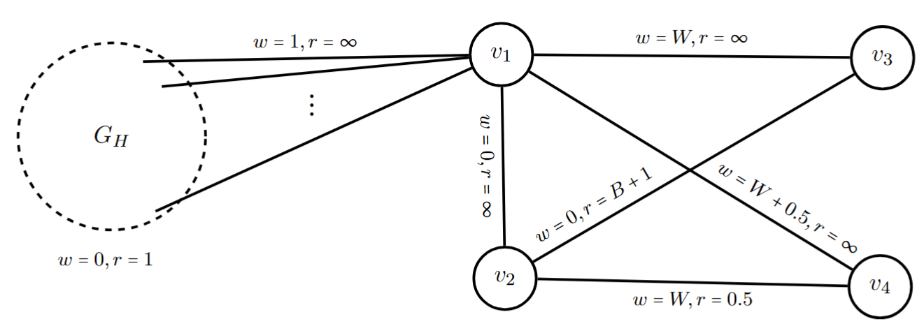
The algorithm chooses the best among the three options:

1.

Return a spanning tree with weight of at least $w_{k}=W+\frac{1}{2}$ (the smallest weight so that the graph without heavier edges is still connected under any removal of edges within the budget $B+\frac{1}{2}$ ). In our example this solution is obtained by removing $(v_{2},v_{4})$ so the MST weight is $W+\frac{3}{2}$ .
2.

Return the empty solution $R_{1}$ (yielding the original minimum spanning tree of weight $W+1$ ).
3.

Return $R$ , the trimmed version of $R_{2}$ . The solution $R$ is created using a reduction to tree knapsack. It holds that $R\subset R_{2}$ , and the cost of $R$ is no more than $B+\frac{1}{2}$ . As $R_{2}=\{(v_{2},v_{3})\}$ , the only subset that does not exceed the profit is $R=\emptyset$ , which again produces the trivial empty solution.

Therefore, in our example the algorithm of [16] chooses the first option, obtaining a solution with spanning tree weight of $W+\frac{3}{2}$ . As the optimal solution is $W+b+\frac{1}{2}$ (and $W>B+1\geq b$ ), the algorithm indeed achieves the promised constant factor guarantee against the total cost of the tree. However, the algorithm achieves a profit of only $\frac{1}{2}$ . The optimal profit is $b-\frac{1}{2}$ , which can be arbitrarily large compared to $\frac{1}{2}$ , depending on maximum components solution in $G_{H}$ .

7 The $\varepsilon$ -Protection Problem

The analysis in Section 3 implies a good defense against $\varepsilon$ -increase. Before presenting the algorithm, we first formalize the problem. The input is a graph $G=(V,E)$ , another set of edges $E^{\prime}$ over $V$ , edge weights $w:E\cup E^{\prime}\rightarrow\mathbb{R}^{+}$ , edge construction costs $b:E^{\prime}\rightarrow\mathbb{R}^{+}$ , and edge removal costs $c:E\cup E^{\prime}\rightarrow\mathbb{R}^{+}$ . For a graph $G$ , let $F^{*}(G)$ denote an optimal solution to the $\varepsilon$ -increase problem discussed above. Our goal in the $\varepsilon$ -protection problem is to compute a set of edges $S\subset E^{\prime}$ to add to $G$ so that $c(F^{*}(G\cup S))>c(F^{*}(G))$ , minimizing the building cost $b(S)$ . We assume that adding any edge $e\in E^{\prime}$ to $G$ does not reduce the weight of a minimum spanning tree. Also, we allow parallel edges (so, for instance, pairs of nodes may be connected by an edge in $E$ and also by an edge in $E^{\prime}$ ).

Based on the algorithm for $\varepsilon$ -increase here is a simple approximation algorithm for this problem. The first step is to list all the partial cuts that the $\varepsilon$ -increase algorithm considers, which have optimal cost. Notice that every cut that the algorithm computes is derived from a global minimum cut of a subgraph of $G$ . In that subgraph, there are at most $\binom{|V|}{2}$ global minimum cuts, and those cuts can be enumerated efficiently. The number of subgraphs to consider is $n-1$ . Thus, the number of listed cuts is less than $n^{3}$ . We want to add at least one edge from $E^{\prime}$ to every listed partial cut. It is possible to approximate an optimal solution within a factor of $O(\log n)$ using the greedy approximation for weighted SET COVER. Simply, associate with each edge in $E^{\prime}$ the set of partial cuts it increases their cost, and then approximate the minimum $b$ -weight set of edges that covers all listed cuts.

References

[1] G. Amanatidis, F. Fusco, P. Lazos, S. Leonardi, A. Marchetti-Spaccamela, and R. Reiffenhäuser. Submodular maximization subject to a knapsack constraint: Combinatorial algorithms with near-optimal adaptive complexity. In Proc. of the 38th Int’l Conf. on Machine Learning, volume 139 of Proceedings of Machine Learning Research, pages 231–242. PMLR, 18–24 July 2021. URL: http://proceedings.mlr.press/v139/amanatidis21a.html.
[2] A. Atamtürk and A. Bhardwaj. Supermodular covering knapsack polytope. Discrete Optimization, 18:74–86, 2015. doi:10.1016/J.DISOPT.2015.07.003.
[3] G. Baier, T. Erlebach, A. Hall, E. Köhler, P. Kolman, O. Pangrác, H. Schilling, and M. Skutella. Length-bounded cuts and flows. ACM Trans. Algorithms, 7(1), 2010. doi:10.1145/1868237.1868241.
[4] C. Bazgan, S. Toubaline, and D. Vanderpooten. Efficient algorithms for finding the $k$ most vital edges for the minimum spanning tree problem. In Proc. of the 5th Ann. Int’l Conf. on Combinatorial Optimization and Applications, pages 126–140, 2011.
[5] C. Bazgan, S. Toubaline, and D. Vanderpooten. Critical edges for the assignment problem: Complexity and exact resolution. Oper. Res. Lett., 41(6):685–689, 2013. doi:10.1016/J.ORL.2013.10.001.
[6] M. Dinitz and A. Gupta. Packing interdiction and partial covering problems. In Proc. of the 16th Int’l Conf. on Integer Programming and Combinatorial Optimization, volume 7801 of Lecture Notes in Computer Science, pages 157–168. Springer, 2013. doi:10.1007/978-3-642-36694-9_14.
[7] M. Feldman, J. Naor, and R. Schwartz. A unified continuous greedy algorithm for submodular maximization. In Proc. of the 52nd Ann. IEEE Symp. on Foundations of Computer Science, pages 570–579, 2011.
[8] G. N. Frederickson and R. Solis-Oba. Increasing the weight of minimum spanning trees. In Proc. of the 7th Ann. ACM-SIAM Symp. on Discrete Algorithms, pages 539–546, 1996.
[9] G. Gallo and B. Simeone. On the supermodular knapsack problem. Math. Program., 45(1–3):295–309, 1989. doi:10.1007/BF01589108.
[10] M. X. Goemans and J. A. Soto. Algorithms for symmetric submodular function minimization under hereditary constraints and generalizations. SIAM J. Discret. Math., 27(2):1123–1145, 2013. doi:10.1137/120891502.
[11] J. Guo and Y. R. Shrestha. Parameterized complexity of edge interdiction problems. In Proc. of the 20th Int’l Conf. on Computing and Combinatorics, volume 8591 of Lecture Notes in Computer Science, pages 166–178. Springer, 2014. doi:10.1007/978-3-319-08783-2_15.
[12] S. Haney, B. Maggs, B. Maiti, D. Panigrahi, R. Rajaraman, and R. Sundaram. Symmetric interdiction for matching problems. In In Proc. of the 20th Int’l Workshop on Approximation Algorithms for Combinatorial Optimization Problems, volume 81 of Leibniz International Proceedings in Informatics (LIPIcs), pages 9:1–9:19. Schloss Dagstuhl – Leibniz-Zentrum für Informatik, 2017. doi:10.4230/LIPICS.APPROX-RANDOM.2017.9.
[13] R. Iyer and J. Bilmes. Submodular optimization with submodular cover and submodular knapsack constraints. In Proc. of the 26th Int’l Conf. on Neural Information Processing Systems, pages 2436–2444, 2013.
[14] L. Khachiyan, E. Boros, K. Borys, K. M. Elbassioni, V. Gurvich, G. Rudolf, and J. Zhao. On short paths interdiction problems: Total and node-wise limited interdiction. Theory Comput. Syst., 43(2):204–233, 2008. doi:10.1007/S00224-007-9025-6.
[15] E. Liberty and M. Sviridenko. Greedy minimization of weakly supermodular set functions. In Approximation, Randomization, and Combinatorial Optimization. Algorithms and Techniques (APPROX/RANDOM 2017), volume 81 of Leibniz International Proceedings in Informatics (LIPIcs), pages 19:1–19:11, 2017. doi:10.4230/LIPICS.APPROX-RANDOM.2017.19.
[16] A. Linhares and C. Swamy. Improved algorithms for MST and metric-TSP interdiction. In Proc. of the 44th Int’l Colloq. on Automata, Languages, and Programming, volume 80 of LIPIcs, pages 32:1–32:14. Schloss Dagstuhl – Leibniz-Zentrum für Informatik, 2017. doi:10.4230/LIPICS.ICALP.2017.32.
[17] K. Liri and M. Chern. The most vital edges in the minimum spanning tree problem. Inform. Proc. Lett., 45:25–31, 1993. doi:10.1016/0020-0190(93)90247-7.
[18] M. Sviridenko. A note on maximizing a submodular set function subject to a knapsack constraint. Oper. Res. Lett., 32(1):41–43, 2004. doi:10.1016/S0167-6377(03)00062-2.
[19] M. Sviridenko, J. Vondrák, and J. Ward. Optimal approximation for submodular and supermodular optimization with bounded curvature. In Proc. of the 26th Ann. ACM-SIAM Symp. on Discrete Algorithms, pages 1134–1148, 2015.
[20] Z. Svitkina and L. Fleischer. Submodular approximation: Sampling-based algorithms and lower bounds. In Proc. of the 49th Ann. IEEE Symp. on Foundations of Computer Science, pages 697–706, 2008.
[21] usul (https://cstheory.stackexchange.com/users/8243/usul). Maximizing a monotone supermodular function s.t. cardinality. Theoretical Computer Science Stack Exchange. URL: https://cstheory.stackexchange.com/q/33967 (version: 2016-03-03).
[22] J. Vondrák, C. Chekuri, and R. Zenklusen. Submodular function maximization via the multilinear relaxation and contention resolution schemes. In Proc. of the 43rd Ann. ACM Symp. on Theory of Computing, pages 783–792, 2011.
[23] R. Zenklusen. Matching interdiction. Discret. Appl. Math., 158:1676–1690, 2008.
[24] R. Zenklusen. An ${O}(1)$ -approximation for minimum spanning tree interdiction. In Proc. of the 56th Ann. IEEE Symp. on Foundations of Computer Science, pages 709–728, 2015.

Appendix A Proofs Appendix

Proof of Lemma 1.

In this proof, we will use the so-called blue rule, which states the following: suppose you have a graph $G$ and some of the edges of a minimum spanning tree are colored blue. If you take any complete cut $C$ of $G$ that contains no blue edge, and any edge $e\in C$ of minimum weight, then there exists a minimum spanning tree of $G$ that contains all the blue edges and $e$ . Consider the edges $e\in T\setminus F$ in arbitrary order. The complete cuts $C_{e}=C_{T,e}$ are disjoint. Also, such an edge $e$ has minimum weight in $C_{e}$ , and therefore also minimum weight in $C_{e}\setminus F$ . Thus, we can use the blue rule repeatedly in $G^{\prime}$ to color all the edges in $T\setminus F$ blue. $\hfill\blacktriangleleft$

Proof of Lemma 2.

If $W\leq w(e)$ then the claim is trivial, as the profit of a cut is non-negative. Thus, we may assume that $W>w(e)$ . Moreover, the worst case is when $e$ has minimum weight in $C_{G}(S)$ , because if the claim holds for a minimum weight edge then it holds also for all edges. Clearly, if $e=(u,v)$ is a minimum weight edge in $C_{G}(S)$ , then there exists a minimum spanning tree $T$ of $G$ that contains $e$ (apply the blue rule to $C_{G}(S)$ and $e$ ). Let $T$ be a minimum spanning tree of $G$ satisfying $e\in T$ , and let $T^{\prime}$ be a minimum spanning tree of $G\setminus C$ . As $e\in C_{G}(S)$ and $W>w(e)$ , it holds that $e\notin T^{\prime}$ . By adding $e$ to the tree $T^{\prime}$ , we create a cycle $P$ . As $e\in P$ crosses $C(S)$ , there must be another edge $e^{\prime}\in P$ that crosses $C_{G}(S)$ . Clearly, $e^{\prime}\in T^{\prime}$ because the only edge in $P\setminus T^{\prime}$ is $e$ . It holds that $w(e^{\prime})\geq W$ , because otherwise $e^{\prime}\in C$ and therefore not in $T^{\prime}$ . Assume for contradiction that $c(T^{\prime})<c(T)+W-w(e)$ . Replacing $e^{\prime}$ with $e$ we create a new spanning tree $T^{\prime\prime}$ of $G$ of weight $c(T^{\prime\prime})\leq c(T^{\prime})-w(e^{\prime})+w(e)\leq c(T^{\prime})-W+w% (e)<c(T),$ a contradiction to the fact that $T$ is a minimum spanning tree of $G$ . Thus, it holds that $c(T^{\prime})\geq c(T)+W-w(e)$ , and therefore $p_{G}(C)\geq W-w(e)$ . $\hfill\blacktriangleleft$

Proof of Lemma 3.

If $G\setminus B\setminus\{e\}$ is not connected, then as $G\setminus B$ is connected by assumption, we have $p_{G\setminus B}(e)=\infty\geq p_{G}(e)$ , so the lemma holds. Thus, we may assume that $G\setminus B\setminus\{e\}$ (and therefore also $G\setminus\{e\}$ ) is connected. Let $e=\{u,v\}$ . We set $W$ to be the maximum over all $u$ - $v$ cuts in $G\setminus\{e\}$ of the minimum weight edge crossing the cut. More formally,

W=\max\{\min\{w(e^{\prime}):\ e^{\prime}\in C_{G\setminus\{e\}}(S)\}:\ S% \subset V\wedge|\{u,v\}\cap S|=1\}.

We show that if $W\geq w(e)$ , then $p_{G}(e)=W-w(e)$ . By Lemma 2 we have $p_{G}(e)\geq W-w(e)$ , so it suffices to prove the reverse inequality. Let $T$ be an arbitrary minimum spanning tree of $G$ . If $e\not\in T$ , then every edge $e^{\prime}$ on the path in $T$ connecting $u$ and $v$ must have $w(e^{\prime})\leq w(e)$ , hence $W\leq w(e)$ and the claim holds vacuously if $W<w(e)$ and as $p_{G}(e)=0$ if $W=w(e)$ . Otherwise, if $e\in T$ , then by Lemma 1, there exists a minimum spanning tree $T^{\prime}$ of $G\setminus\{e\}$ so that $T^{\prime}=T\cup\{e^{\prime}\}\setminus\{e\}$ for an edge $e^{\prime}\in E$ . In particular, $e^{\prime}\in C_{T,e}$ is the minimum weight edge in this cut, and the partial cut $\{e^{\prime\prime}\in C_{T,e}:\ w(e^{\prime\prime})<w(e^{\prime})\}$ is a candidate cut. Therefore $W\geq w(e^{\prime})$ and $p_{G}(e)=w(e^{\prime})-w(e)\leq W-w(e)$ . Now, if $p_{G}(e)=0$ then the assertion of the lemma is trivial. Otherwise, if $p_{G}(e)>0$ , then $e$ must be contained in every minimum spanning tree of $G$ . By the above characterization of $p_{G}(e)$ , we have that $p_{G}(e)=W-w(e)$ , where $W$ is a minimum weight of an edge in some cut $C_{G\setminus\{e\}}(S)$ . As $C^{\prime}=C_{G\setminus B\setminus\{e\}}(S)\subset C_{G\setminus\{e\}}(S)$ , we have that $W^{\prime}=\min\{w(e^{\prime}):\ e^{\prime}\in C^{\prime}\}\geq W$ . Using the same characterization of $p_{G\setminus B}(e)$ , we get $p_{G\setminus B}(e)\geq W^{\prime}-w(e)\geq W-w(e)=p_{G}(e)$ . $\hfill\blacktriangleleft$

Proof of Corollary 4.

This is a simple application of Lemma 3, removing the edges of $A=\{e_{1},\ldots e_{k}\}$ one by one. Denote $A_{0}=\emptyset$ , $A_{1}=\{e_{1}\}$ , $\dots$ , $A_{i}=\{e_{1},e_{2},\dots,e_{i}\}$ , $\dots$ , $A_{k}=\{e_{1},e_{2},\dots,e_{k}\}$ . By Lemma 3, for every $i=1,2,\dots,k$ , it holds that $p_{G\setminus B\setminus A_{i-1}}(e_{i})\geq p_{G\setminus A_{i-1}}(e_{i}).$ Therefore, $p_{G\setminus B}(A)=\sum_{i=1}^{k}p_{G\setminus B\setminus A_{i-1}}(e_{i})\geq% \sum_{i=1}^{k}p_{G\setminus A_{i-1}}(e_{i})=p_{G}(A),$ which completes the proof. $\hfill\blacktriangleleft$

Proof of Claim 5.

We show that the optimal solution $F^{*}$ is achieved at a partial cut considered by the algorithm, and therefore the claim follows. If $F^{*}$ disconnects $G$ , then it is a global MIN CUT with respect to the edge costs $c$ . Moreover, all the edges in this cut have the same weight, otherwise removing just the lightest edges would increase the weight of the minimum spanning tree, at lower cost. Therefore, if the algorithm deals with one of the edges $e\in F^{*}$ , one of the feasible cuts it minimizes over is $F^{*}$ . Because $T$ is a spanning tree it must have at least one edge in any complete cut in the graph, and specifically in $F^{*}$ . In fact, in this case the algorithm will output either $F^{*}$ or another global MIN CUT of the same cost. If $F^{*}$ does not disconnect $G$ we argue as follows. Let $T^{\prime}$ be a minimum spanning tree of $G\setminus F^{*}$ . Recall that for every $e\in T\setminus T^{\prime}$ there exists $e^{\prime}\in(T^{\prime}\setminus T)\cap C_{T,e}$ such that $T-e+e^{\prime}$ is a spanning tree. Let’s consider the edges $e\in T\setminus T^{\prime}$ in arbitrary order, and let’s choose $e^{\prime}=\pi(e)$ that minimizes $w(e^{\prime})$ among all edges in $(T^{\prime}\setminus T)\cap C_{T,e}$ . Let $e_{1}$ denote the first edge considered in $T\setminus T^{\prime}$ . As $T$ is a minimum spanning tree, $w(\pi(e_{1}))\geq w(e_{1})$ . Denote $T_{0}=T$ and $T_{1}=T-e_{1}+\pi(e_{1})$ . If $w(\pi(e_{1}))=w(e_{1})$ , we can repeat this argument with $T_{1}$ and $T^{\prime}$ to get $T_{2}$ , and so forth. This process must reach an iteration $i\leq|T\setminus T^{\prime}|$ at which $w(\pi(e_{i}))>w(e_{i})$ , otherwise $w(T^{\prime})=w(T)$ , in contradiction to the definition of $F^{*}$ . Now, consider the cut $C_{T_{i-1},e_{i}}$ in $G$ . Notice that by construction, $T_{i-1}$ is also a minimum spanning tree of $G$ , because all exchanges prior to step $i$ did not increase the weight of the tree. Thus, $w(e_{i})$ is the minimum length of an edge in this cut. Also, $\pi(e_{i})$ is an edge in this cut. By our choice of $\pi(e_{i})$ , none of the edges in the set $F=\{e^{\prime}\in C_{T_{i-1},e_{i}}:\ w(e^{\prime})<w(\pi(e_{i}))\}$ are in $T^{\prime}$ . If there exists $e^{\prime}\in F\setminus F^{*}$ , then the cycle closed by adding $e^{\prime}$ to $T^{\prime}$ must contain at least one other edge $e^{\prime\prime}\in T^{\prime}\cap C_{T_{i-1},e_{i}}$ . However, all such edges have $w(e^{\prime\prime})>w(e^{\prime})$ , in contradiction to the assumption that $T^{\prime}$ is a minimum spanning tree of $G\setminus F^{*}$ . Thus, $F\subseteq F^{*}$ .

Now, consider $F^{\prime}\subseteq F$ , putting $F^{\prime}=\{e^{\prime}\in C_{T_{i-1},e_{i}}|w(e^{\prime})=w(e_{i})\}$ . Let $T^{\prime\prime}$ be a minimum spanning tree of the graph $G\setminus F^{\prime}$ . Clearly, $w(T^{\prime\prime})>w(T)$ and $c(F^{\prime})\leq c(F^{*})$ . Hence, $F^{\prime}$ is an optimal solution which contains all the minimum-weight edges in the cut $C_{T_{i-1},e_{i}}$ . Let’s assume in contradiction that the minimum spanning tree $T$ that the algorithm chooses and iterates over its edges maintains $T\cap F^{\prime}=\emptyset$ . Then there exists an edge $e\in T$ , with $w(e)>w(e_{i})$ that crosses the cut, and we can replace it and create lighter spanning tree as $w(T-e+e_{i})<w(T)$ . This contradict $T$ being a minimum spanning tree. We conclude that there is an edge $e\in T\cap F^{\prime}$ . Therefore, $F^{\prime}$ is one of the cuts that the algorithm optimizes over when considering $e$ . The algorithm may choose a different cut for $e$ , but the chosen cut will not have cost greater than $c(F^{\prime})$ . $\hfill\vartriangleleft$

Proof of Claim 6.

In this proof, we will use repeatedly the blue rule; see the proof of Lemma 1 for details. Consider the best $e$ and the corresponding cut $C$ that determines the output of the algorithm. There exists a minimum spanning tree $T$ of $G$ that contains $e$ , because we can apply the blue rule to $C$ and $e$ . Let $S$ be the forest that remains of $T$ after removing all the edges of length $w(e)$ in $C$ . Clearly, $S$ has at least two connected components, at least one on each side of the cut $C_{T,e}$ (be aware that this cut may differ from $C$ ). If the new graph is disconnected, then clearly the claim holds. Otherwise, $S$ can be extended to a minimum spanning tree $T^{\prime}$ of the new graph, as we can use the blue rule to color blue each edge $f\in S$ , using the cut $C_{T,f}$ that does not contain any other edge of $T$ (Clearly $f$ has minimum length in this cut prior to the removal of edges, and therefore also after the removal of edges).

Let’s assume for contradiction that $w(T^{\prime})=w(T)$ . Let $P$ be the cycle created by adding $e$ to $T^{\prime}$ . As $e$ crosses $C$ , there must be another edge $e\in P$ that crosses $C$ . We must have that $w(e^{\prime})>w(e)$ , as we eliminated from $C$ all the edges of length $w(e)$ . By the assumption, it must be that $e^{\prime}\in T$ , otherwise $w(T^{\prime})>w(T)$ (exchanging $e^{\prime}$ with $e$ reduces the cost of the tree, but $T$ is a minimum spanning tree of $G$ ). Consider now $C_{T,e^{\prime}}$ . As $e^{\prime}$ crosses $C_{T,e^{\prime}}$ , there must be another $e^{\prime\prime}\in P$ that crosses $C_{T,e^{\prime}}$ . However, $e^{\prime\prime}\not\in T$ , because $C_{T,e^{\prime}}\cap T=\{e^{\prime}\}$ by definition. Thus, by our assumption $w(e^{\prime\prime})=w(e)<w(e^{\prime})$ (for the same reason that, otherwise, exchanging $e^{\prime\prime}$ with $e$ reduces the length of $T^{\prime}$ , but we assumed that $w(T^{\prime})=w(T)$ and $T$ is a minimum spanning tree of $G$ ). This is a contradiction to the assumption that $T$ is a minimum spanning tree, together with the implications that $e^{\prime}\in T$ and $e^{\prime\prime}\in C_{T,e^{\prime}}\setminus\{e^{\prime}\}$ . $\hfill\vartriangleleft$

[bib.bib1] [1] G. Amanatidis, F. Fusco, P. Lazos, S. Leonardi, A. Marchetti-Spaccamela, and R. Reiffenhäuser. Submodular maximization subject to a knapsack constraint: Combinatorial algorithms with near-optimal adaptive complexity. In Proc. of the 38th Int’l Conf. on Machine Learning, volume 139 of Proceedings of Machine Learning Research, pages 231–242. PMLR, 18–24 July 2021. URL: http://proceedings.mlr.press/v139/amanatidis21a.html.

[bib.bib2] [2] A. Atamtürk and A. Bhardwaj. Supermodular covering knapsack polytope. Discrete Optimization, 18:74–86, 2015. doi:10.1016/J.DISOPT.2015.07.003.

[bib.bib3] [3] G. Baier, T. Erlebach, A. Hall, E. Köhler, P. Kolman, O. Pangrác, H. Schilling, and M. Skutella. Length-bounded cuts and flows. ACM Trans. Algorithms, 7(1), 2010. doi:10.1145/1868237.1868241.

[bib.bib4] [4] C. Bazgan, S. Toubaline, and D. Vanderpooten. Efficient algorithms for finding the $k$ most vital edges for the minimum spanning tree problem. In Proc. of the 5th Ann. Int’l Conf. on Combinatorial Optimization and Applications, pages 126–140, 2011.

[bib.bib5] [5] C. Bazgan, S. Toubaline, and D. Vanderpooten. Critical edges for the assignment problem: Complexity and exact resolution. Oper. Res. Lett., 41(6):685–689, 2013. doi:10.1016/J.ORL.2013.10.001.

[bib.bib6] [6] M. Dinitz and A. Gupta. Packing interdiction and partial covering problems. In Proc. of the 16th Int’l Conf. on Integer Programming and Combinatorial Optimization, volume 7801 of Lecture Notes in Computer Science, pages 157–168. Springer, 2013. doi:10.1007/978-3-642-36694-9_14.

[bib.bib7] [7] M. Feldman, J. Naor, and R. Schwartz. A unified continuous greedy algorithm for submodular maximization. In Proc. of the 52nd Ann. IEEE Symp. on Foundations of Computer Science, pages 570–579, 2011.

[bib.bib8] [8] G. N. Frederickson and R. Solis-Oba. Increasing the weight of minimum spanning trees. In Proc. of the 7th Ann. ACM-SIAM Symp. on Discrete Algorithms, pages 539–546, 1996.

[bib.bib9] [9] G. Gallo and B. Simeone. On the supermodular knapsack problem. Math. Program., 45(1–3):295–309, 1989. doi:10.1007/BF01589108.

[bib.bib10] [10] M. X. Goemans and J. A. Soto. Algorithms for symmetric submodular function minimization under hereditary constraints and generalizations. SIAM J. Discret. Math., 27(2):1123–1145, 2013. doi:10.1137/120891502.

[bib.bib11] [11] J. Guo and Y. R. Shrestha. Parameterized complexity of edge interdiction problems. In Proc. of the 20th Int’l Conf. on Computing and Combinatorics, volume 8591 of Lecture Notes in Computer Science, pages 166–178. Springer, 2014. doi:10.1007/978-3-319-08783-2_15.

[bib.bib12] [12] S. Haney, B. Maggs, B. Maiti, D. Panigrahi, R. Rajaraman, and R. Sundaram. Symmetric interdiction for matching problems. In In Proc. of the 20th Int’l Workshop on Approximation Algorithms for Combinatorial Optimization Problems, volume 81 of Leibniz International Proceedings in Informatics (LIPIcs), pages 9:1–9:19. Schloss Dagstuhl – Leibniz-Zentrum für Informatik, 2017. doi:10.4230/LIPICS.APPROX-RANDOM.2017.9.

[bib.bib13] [13] R. Iyer and J. Bilmes. Submodular optimization with submodular cover and submodular knapsack constraints. In Proc. of the 26th Int’l Conf. on Neural Information Processing Systems, pages 2436–2444, 2013.

[bib.bib14] [14] L. Khachiyan, E. Boros, K. Borys, K. M. Elbassioni, V. Gurvich, G. Rudolf, and J. Zhao. On short paths interdiction problems: Total and node-wise limited interdiction. Theory Comput. Syst., 43(2):204–233, 2008. doi:10.1007/S00224-007-9025-6.

[bib.bib15] [15] E. Liberty and M. Sviridenko. Greedy minimization of weakly supermodular set functions. In Approximation, Randomization, and Combinatorial Optimization. Algorithms and Techniques (APPROX/RANDOM 2017), volume 81 of Leibniz International Proceedings in Informatics (LIPIcs), pages 19:1–19:11, 2017. doi:10.4230/LIPICS.APPROX-RANDOM.2017.19.

[bib.bib16] [16] A. Linhares and C. Swamy. Improved algorithms for MST and metric-TSP interdiction. In Proc. of the 44th Int’l Colloq. on Automata, Languages, and Programming, volume 80 of LIPIcs, pages 32:1–32:14. Schloss Dagstuhl – Leibniz-Zentrum für Informatik, 2017. doi:10.4230/LIPICS.ICALP.2017.32.

[bib.bib17] [17] K. Liri and M. Chern. The most vital edges in the minimum spanning tree problem. Inform. Proc. Lett., 45:25–31, 1993. doi:10.1016/0020-0190(93)90247-7.

[bib.bib18] [18] M. Sviridenko. A note on maximizing a submodular set function subject to a knapsack constraint. Oper. Res. Lett., 32(1):41–43, 2004. doi:10.1016/S0167-6377(03)00062-2.

[bib.bib19] [19] M. Sviridenko, J. Vondrák, and J. Ward. Optimal approximation for submodular and supermodular optimization with bounded curvature. In Proc. of the 26th Ann. ACM-SIAM Symp. on Discrete Algorithms, pages 1134–1148, 2015.

[bib.bib20] [20] Z. Svitkina and L. Fleischer. Submodular approximation: Sampling-based algorithms and lower bounds. In Proc. of the 49th Ann. IEEE Symp. on Foundations of Computer Science, pages 697–706, 2008.

[bib.bib21] [21] usul (https://cstheory.stackexchange.com/users/8243/usul). Maximizing a monotone supermodular function s.t. cardinality. Theoretical Computer Science Stack Exchange. URL: https://cstheory.stackexchange.com/q/33967 (version: 2016-03-03).

[bib.bib22] [22] J. Vondrák, C. Chekuri, and R. Zenklusen. Submodular function maximization via the multilinear relaxation and contention resolution schemes. In Proc. of the 43rd Ann. ACM Symp. on Theory of Computing, pages 783–792, 2011.

[bib.bib23] [23] R. Zenklusen. Matching interdiction. Discret. Appl. Math., 158:1676–1690, 2008.

[bib.bib24] [24] R. Zenklusen. An ${O}(1)$ -approximation for minimum spanning tree interdiction. In Proc. of the 56th Ann. IEEE Symp. on Foundations of Computer Science, pages 709–728, 2015.

Budget and Profit Approximations for Spanning Tree Interdiction

Abstract

Keywords and phrases:

Category:

Funding:

Copyright and License:

2012 ACM Subject Classification:

DOI:

Event:

Editors:

Series and Publisher:

1 Introduction

Problem statement and results

Motivation

Related work

Our techniques

Organization

2 Preliminaries

Lemma 1.

Lemma 2.

Lemma 3 (super-modularity of the profit function).

Corollary 4.

3 An Algorithm for 𝜺-Increase

Claim 5.

Claim 6.

Corollary 7.

Proof.

4 Relaxed Specification of the Optimum

Theorem 8.

Constructing the sequence of the cuts

Two alternatives

Choosing 𝑿𝒊

Lemma 9.

Proof.

Lemma 10.

Claim 11.

Proof.

Claim 12.

Proof.

Proof of Lemma 10.

Lemma 13.

Claim 14.

Proof of Claim 14.

Claim 15.

Proof.

Claim 16.

Proof.

Proof of Lemma 13.

5 Budget Approximation

Theorem 17.

Lemma 18.

Proof.

Proof of Theorem 17.

Running time

Claim 19.

Proof.

6 Profit Approximation

6.1 Profit approximation algorithm

Theorem 20.

Proof.

Running time

6.2 Bad example for previous algorithms

7 The 𝜺-Protection Problem

References

Appendix A Proofs Appendix

Proof of Lemma 1.

Proof of Lemma 2.

Proof of Lemma 3.

Proof of Corollary 4.

Proof of Claim 5.

Proof of Claim 6.

3 An Algorithm for $\varepsilon$ -Increase

Choosing $X_{i}$

7 The $\varepsilon$ -Protection Problem