Single-Token vs Two-Token Blockchain Tokenomics

Abstract
We study long-term equilibria that arise in the token monetary policy, or tokenomics, design of proof-of-stake (PoS) blockchain systems that engage utility maximizing users and validators. Validators are system maintainers who get rewarded with tokens for performing the work necessary for the system to function properly, while users compete and pay with such tokens for getting a desired portion of the system service.
We study how the system service provision and suitable rewards schemes together can lead to equilibria with the following desirable characteristics (1) viability: the system keeps parties engaged, (2) decentralization and skin-in-the-game: multiple sufficiently invested validators are participating, (3) stability: the price path of the underlying token used to transact with the system does not change widely over time, and (4) feasibility: the mechanism is easy to implement as a smart contract, e.g., it does not require a fiat reserve on-chain to perform token buybacks or to perform bookkeeping of exponentially growing token holdings.
Our analysis enables us to put forward a novel generic mechanism for blockchain monetary policy that we call quantitative rewarding (QR). We investigate how to implement QR in single-token and two-token proof of stake (PoS) blockchain systems. The latter are systems that utilize one token for the users to pay the transaction fees and a different token for the validators to participate in the PoS protocol and get rewarded. Our approach demonstrates a concrete advantage of the two-token setting in terms of the ability of the QR mechanism to be realized effectively and provide good equilibria. Our analysis also reveals an inherent limitation of the single token setting in terms of implementing an effective blockchain monetary policy – a distinction that is, to the best of our knowledge, highlighted for the first time.
Keywords and phrases:
Blockchain, tokenomics, buyback, equilibria, price path, stable price, discounted game, dual-token, proof-of-stake, validatorCopyright and License:
![[Uncaptioned image]](x1.png) © Aggelos Kiayias, Philip Lazos, and Paolo Penna; licensed under Creative Commons License CC-BY 4.0
© Aggelos Kiayias, Philip Lazos, and Paolo Penna; licensed under Creative Commons License CC-BY 4.0
2012 ACM Subject Classification:
Theory of computation Solution concepts in game theoryEditors:
Zeta Avarikioti and Nicolas ChristinSeries and Publisher:
 Leibniz International Proceedings in Informatics, Schloss Dagstuhl – Leibniz-Zentrum für Informatik
1 Introduction
Blockchains create value by offering services in a fully decentralized manner, wherein users pay fees to access these services, while the functioning and security of the system is guaranteed by a set of nodes or validators who receive rewards for performing the necessary computations required by the protocol. These payments are issued in the system’s native token and the mechanism that mints and distributes these tokens to the relevant participants determines the “tokenomics policy” of the blockchain. Designing such policies with good properties is pivotal to ensuring the success of blockchain systems in the long term.
The token’s value or price, denominated in standard (fiat) currency, crucially determines the actual costs for users and the compensation for validators. An upward or downward fluctuation in the token’s price can make the system less attractive for either type of party. While the system cannot directly control its token price in the market, it can implement various monetary policies (such as increasing token minting, burning transaction fees, adjusting the level of transaction fees, change the validator level of rewards, and others) to achieve a long-term equilibrium with the desired price without compromising the system’s viability and decentralization.
This motivates the study of tokenomics design achieving the following important desiderata:
-
1.
Viability. Preconditioned on a positive system value, the system keeps all involved parties actively engaged: validators to guarantee the protocol being live and securely running, and the users to guarantee enough fees are collected at all time.
-
2.
Decentralization and “Skin-in-the-game.” A set of validators each equally engaged in the protocol – maximal decentralization [20], receiving adequate rewards to offset their costs, while also having significant stake in the system operation (e.g. in the case of proof-of-stake (PoS) systems, validators “staking” high enough amount of tokens).
-
3.
Stability. Reasonably stable token prices, meaning that the price of the token required to issue transactions does not significantly change over time.
-
4.
Feasibility. The tokenomics policy should be feasible to implement on-chain algorithmically. In particular, this means that the policy avoids using features that are incompatible or difficult to implement in the form of smart contracts, integrate into the blockchain accounting model or they are antithetical to blockchain decentralization. For example, the policy should minimize the use of off-chain entities that need to intervene actively to adjust policy (e.g., a central bank type of actor), or the use of techniques such as buybacks which would require a fiat reserve to facilitate. Furthermore, all the numerical quantities that are accounted in the ledger (e.g., the number of tokens held by a validator) should not grow exponentially over time.
The conditions under which there is a tokenomics policy achieving all these requirements is a fundamental question which we address in this work.
1.1 Main contributions
We explore tokenomics policies in the PoS setting, i.e., the setting where validators have to acquire tokens and stake them in order to receive rewards and perform the necessary system maintenance to further the system’s operation. We put forth a model where a set of users and validators engage with the system in discrete time steps. At each time step, users and validators buy or sell tokens in order to accommodate their objectives that include issuing transactions and staking tokens to provide the service.
Modeling framework.
The model takes as given two exogenous parameters. The discount factor , a conventional element in economic models, reflects players’ preference for immediate utility over future gains, and is tied to the risk-free rate. The value of the service captures the usefulness of the system for users in each round and may fluctuate unpredictably due to external shocks (Remark 3). The system can set rewards to be distributed in each round to the validators according to their current stake at round ; each validator also faces a fixed cost associated with maintaining the required secure node configuration. As our analysis shows, the monetary policy, , influences the equilibrium and the token price. One of our key findings (see below) is that suitably defined monetary policies can “absorb” shocks and avoid undesirable price fluctuations.
The equilibria in our model come from players who aim to maximize their own discounted utility, thus choosing strategies with time-dependent parameters, such as how many tokens to sell on the market or retain for future rounds (users need to spend tokens to access the system, while validators need to stake tokens to receive rewards). These equilibria, in turn, govern the key endogenous variables of the system, namely the staking levels of the validators, the holdings of user tokens, the fees paid to the system, the demand and supply of tokens in the spot market and the resulting trajectory or price path of the token (the market-clearing price in equilibrium as in [11]).
Equilibria analysis and quantitative rewarding.
We give both boundary conditions and actual policies (mechanisms) that implement equilibria with all desired features: viability, decentralization, stability, and feasibility. Specifically, our analysis leads us to put forward a novel generic mechanism for blockchain “monetary policy”:
Quantitative Rewarding (QR). The amount of rewards the system gives to the validators is suitably adjusted at each step to anticipate changes in the value of the service.
This QR concept arises from our equilibrium analysis, focusing on how market demand and supply respond to changes in service value and rewards . In all equilibria implementing certain desired price paths, the following conditions hold at every round (cf. Theorem 9):
-
Users spend an amount of tokens whose value is a constant fraction of the current service value .
-
Validators stake an amount of tokens that is a constant fraction of current rewards .
As these conditions and equilibria do not rule out undesirable mechanisms such as buybacks, our goal is to use QR to induce equilibria where token demand and supply match–so no buybacks are needed. Observe that if, at any point in time, the value of the service decreases, users will buy fewer tokens, thus reducing demand and threatening price stability. Instead of relying on buybacks, our QR mechanism, perhaps somewhat counterintuitively, increases the rewards allocated to validators, who react by staking more tokens, which must be acquired from the market. This action effectively restores the demand for tokens to align with the supply. The reverse effect occurs when the value of the service increases.
We show that implementing QR in single-token systems to avoid buybacks is highly non-trivial, as it requires anticipating future shocks far in advance. In contrast, for two-token systems, QR can be implemented using only a one-step lookahead of the service value. This conclusion stems from equilibrium analysis, but can be intuitively explained as follows: In single-token systems, validators must retain some tokens to stake and sell only a portion to the market to satisfy demand. In two-token systems, one token is used for staking, while the other – distributed as rewards in our mechanism – is used by users. Validators can sell all of these reward tokens to the market, making it easier to align supply with demand. Consequently, any equilibrium where rewards match the next round’s service value (current users’ demand for new tokens) avoids buybacks.
Decoupling users from validators via distinct tokens enables the system to absorb service value fluctuations more effectively, while keeping the user token’s price stable and preserving other desiderata. At equilibrium, the price of the stake token rises gradually, and validators stake a fixed amount, trading only the other token, which they receive as a reward. In contrast, a single-token setup may trigger a self-reinforcing loop of increasing validator rewards, even after service levels stabilize, underscoring a fundamental distinction between the single-token and two-token configurations.
Implementing QR and its challenges.
In Section 3.3, we investigate how to implement QR via a mechanism which adjusts the rewards at every round based on the current rewards and the next round service value using a single token for accounting. An important challenge that arises in this setting is that the rewards formula is subject to a recursive condition (see the lower bound in Theorem 13 and Corollary 14) which makes rewards subject to a “feedback loop” effect that can lead to rewards explosion.
As a result, while maintaining certain (minimal) rewards to ensure decentralization and security, it is possible that the system can trigger an uncontrolled growth in the amount of rewards distributed and in the staked amounts of tokens (see Section 3.3.1 for conditions that trigger such explosion). In Section 3.4 we describe in detail the implementation of our mechanism for the case of stable prices. This implementation includes the strategies for users and validators, showing that all information needed is service value at the next round (despite their simplicity, these strategies still constitute an equilibrium in the underlining repeated game, i.e., when more complex time-dependent strategies are in principle possible).
The above results apply to the single token setting which is the most common in PoS systems (e.g., Ethereum and Cardano operate in this way, for example, as PoS cryptocurrencies) and paint a rather negative picture: one has to either accept tokenomics with widely fluctuating token prices (the most common outcome that is observed in these systems as deployed in the real world), implement drastic measures such as token buybacks, or suffer a potential explosion in rewards accounting (unless future shocks in service value can be predicted – a rather unreasonable assumption). Note that QR mechanisms are, in general, more complex than standard “fee burning” policies used in practice (see Remark 16).
Two-token systems and QR.
Poised to obtain a more favorable outcome, we next explore the implementation of QR in two token PoS systems in which one token is used to get the service and another token is used for staking (and governance). While less common, this type of setup has been adopted in a few occasions: e.g., in the NEO cryptocurrency [19] and can be implemented in other systems as well (e.g., in the Cosmos SDK [8]). To investigate the potential of QR in this setting, we adapt our model to the two tokens setting (Section 4). In order to maintain feasibility, while maintaining desirable prices, we identify the necessary conditions that equilibria (mechanism) must guarantee in terms of rewards.
The two token mechanism for QR is presented in Section 4.3. The main advantage of the resulting rewards formula is that it is simpler than in the single token setting and the mechanism does not need to know “global information” about the service value time series – merely a one step lookahead suffices (cf. Theorem 24). As an important corollary, the mechanism achieves our objectives and is capable of avoiding the feedback loop effect of the single token case that leads to an exponential explosion for rewards.
1.2 Related work
In the single-token setting, our results build on the model of [11]. In [11], the author considers a platform design framework in which the system designer selects both time-dependent rewards and service quality . There, is not influenced by external shocks; rather, it is deterministically set by the system, which incurs a cost depending on the chosen service quality. Market frictions are captured through shocks occurring at the user level: with a fixed probability, token holdings are reset to zero at each round. The objective is to maximize system profit, and the platform is permitted to engage in the spot market, either by selling or buying back tokens. Compared to that prior work, our results accommodate a more general class of equilibria as [11] uses a “rigid” policy that needs buybacks (see full version [15] for details). To the best of our knowledge, ours is the first analytical model for such systems to study their equilibria and related token price paths achieving all four desiderata we set out in the beginning of this section. Other prior work includes the effects of tokens regarding user adoption and equilibrium selection [1, 2, 18], or using token supply to promote optimal growth and service provision [6], also allowing (costly) buybacks [7] that cause underinvestment in productivity. Different aspects of the monetary characteristics of tokens have been studied in [25, 21, 22], while [16] considered token burning; notably one can view QR as a generalization of the token burning mechanism that is more versatile, cf. 16. In prior work, typically users receive the most attention, but [4] expand on the strategy space of validators and their alternative uses for tokens. Further work modeling validators’ staking strategies are [5, 13, 24, 14]. While all previous work has focused on the single token design, [9] considered two-token systems and proposed several economic indicators (most of them depending on the prices of the two tokens, and thus our price analysis at equilibrium can be combined with these proposed metrics).
2 Model description and notation (single token)
Notation (single token model)
-
= number of users (fixed and constant over time).
-
= number of validators (fixed and constant over time).
-
= token holding of a generic player (user or validator).
-
= price of the token.
-
the value of a generic quantity at time .
-
= discounted version of quantity , that is, .
-
= generalization of the previous definition in which we start at and discount accordingly, that is, .
-
= validator ’s selling strategy at time (negative values are possible, i.e., buying).
-
= user ’s buying strategy at time (negative values are possible, i.e., selling).
-
= amount of tokens that user pays for the service at time .
-
= cost incurred by each validator (identical for all validators and all ).
-
is the total reward for validators at time , which is further distributed to each validator according to a reward sharing scheme , meaning that validator receives an amount of tokens equal to
(1) where are the token holding of all validators but .
-
is the service value at time , which is further divided among the users according to some scheme , meaning that each user receives a service value
(2) where are the used tokens of all users but .
-
= generic non-decreasing decentralization factor, where is the number of validators.
-
= instantaneous utility of user , given by
(3) -
= instantaneous utility of validator , given by
(4)
We consider a Lagos-Wright ([17]) type of model, in which there are two kinds of players: users and validators, as in [16, 11]. We have a repeated game where each round , consists of two phases or subrounds. Players first interact with the system (users pay the system to get some service, and validators stake tokens to access rewards for performing some task), and then they interact with a “spot market” (players buy or sell their tokens at the end of the round in order to hold the amount of tokens they need at the next round). In order to describe the model in detail, we introduce some notation in Figure 1. The two subrounds are as follows:
Subround I (pay & stake)
Each user and each validator has and tokens, respectively. Then, given some (total) value of the service and the total rewards for validators, we have
-
1.
Each validator performs some work, incurs a cost , and receives an amount of additional tokens according to Equation (1), given the total reward for validators .
-
2.
Each user uses some of her currently available tokens to pay for the service, and receives the corresponding service value according to Equation (2), given the value of the service .
Subround II (buy or sell)
Each user and each validator has and tokens, respectively. Both type of players (users and validators) can buy any amount of new tokens or sell (part or all of the tokens they currently have) at the current market price. In detail:
-
1.
Each validator sells tokens to the market and receives units of money in return. Note that we have a validator’s selling constraint
(5) Any negative is allowed, meaning that is actually buying tokens from the market at the current price.
-
2.
Each user buys additional tokens from the market and pays units of money for that. Any negative is allowed, meaning that is selling tokens to the market at the current price. Note that we have a users’s selling constraint
(6)
At the end of subround II of step we get the token holdings for the next step, , for each user and each validator , respectively
| (7) |
Each user and each validator aims at maximizing her own discounted utility, respectively
| (8) | ||||
| (9) |
subject to their respective selling constraints in (6) and in (5). As usual, the discount factor above is where is the risk free rate.111Intuitively, the system is analyzed as investment “against” the risk-free investment which is captured abstractly by the risk-free rate. Also, at equilibrium validators do not necessarily break even (as e.g., in prior work [11]) but they can have positive utility at each step, cf. Section 4.3.
Definition 1 (symmetric equilibrium).
Consider a system policy given by (1) and (2), and a triple of users’ strategies, validators’ strategies, and prices
such that the corresponding selling constraints (6) and (5) are satisfied. We say that such a triple is an equilibrium if
-
1.
Strategy maximizes the discounted utility (9) of validator , given all other strategies, for each validator ;
-
2.
Strategy maximizes the discounted utility (8) of user , given all other strategies, for each user ;
-
3.
The resulting two sequences of token holdings (7) are strictly positive, that is, and .
Moreover, we say that such an equilibrium is symmetric if the token holdings of all users are the same, and similarly, if all token holdings of all validators are the same, correspond to sequences of strictly positive token holdings
| (10) |
for all users and for all validators and for all .
We should point out that, in addition to being natural, the symmetry conditions (10) are often without loss of generality (see full version [15] for details).
Remark 2 (viability and equilibria).
In order to establish the existence of equilibria, we need a few (technical) assumptions, regarding the service value (Assumption 1) and about the rewards and service sharing functions (Assumption 2 below).
Assumption 1 (service value).
The service value is upper bounded by some (arbitrarily large) constant independent of .
The value of the constant in Assumption 1 does not affect the results and bounds in any way, and is only needed to establish the existence of equilibria. Other than this, we make no other assumptions, and allow to increase or decrease arbitrarily within this range.
Remark 3 (service value fluctuations – shocks).
The service value represents the overall value the system provides to users. Several factors (technological improvements, competitors, regulations, market conditions) influence . Consequently, the system may neither fully control nor predict all future values of , as these factors can cause unforeseen shocks.
3 Single token mechanisms
3.1 Analysis of price path
In this section we provide the analysis of the prices for the following family of service allocation and rewards:
| (11) |
where and are arbitrary differentiable functions in , and where the indexes and in the summations range over all users and all validators, respectively. In the following, we denote by and the first derivatives of and , respectively. We make the following assumption about and .
Assumption 2.
Lemma 4.
In any symmetric equilibrium, it holds that
| (12) |
Moreover
| (13) |
Hence, if , then and for all users , and the following identity must hold:
| (14) |
A simple class of schemes satisfying our assumptions is the following one from [11]:
| (15) |
Example 5 below provides another possible reward sharing function other than the one in (15). We do not claim that this alternative provides any particular improvement, but simply point out that changing , and similarly , does affect the equilibria as described by Lemma 4 (see full version [15] for further examples and discussion).
Example 5.
For any parameter , the following reward sharing function satisfies , meaning that for smaller number of validators a smaller fraction of the total allocated rewards is actually distributed. Since , we have for sufficiently large .
Remark 6.
Assumption 2 implies that whenever , thus implying that the largest possible price growth must satisfy where and is the risk-free rate. Intuitively, the return rate for just holding the token cannot beat the risk-free rate, as one might expect when looking for equilibria that keep all users and validators engaged (viability). Whether blockchains can achieve return rates competitive with the inflation is studied in [10] in relation to policies adopted by some of the current blockchains, though without providing analytical results.
3.2 Generic symmetric equilibria
In the following we focus on the interesting case of prices having a constant multiplicative growth, which includes stable prices as a special case.
Definition 7 (-stable prices).
We say that the prices (of some equilibrium under consideration) are -stable if, for all , they satisfy
| (16) |
Note that stable prices satisfy the above condition with , while and correspond to decreasing and increasing prices, respectively.
We next define a class of generic symmetric equilibria which, as we prove below, captures all symmetric equilibria with -stable prices.
Definition 8 (generic symmetric equilibrium).
A symmetric equilibrium is generic if the following conditions hold for all and constants :
-
1.
The monetary amount of tokens that users hold (and use) is proportional to the value of the service offered by the system. That is, the service to fees ratio is constant,
-
2.
The amount of tokens staked by validators is proportional to the rewards offered by the system. That is, the rewards to stake ratio is constant,
-
3.
The prices satisfy
where constants and depend only on the number of users , the number of validators , the rewards sharing scheme, and on the service fee scheme.
-
4.
Each user starts round with the same token holding , uses all its token current holding for the service (), and buys new tokens needed for the next round accordingly ().
Note that generic symmetric equilibria provide additional structure to the definition of symmetric equilibria. The following theorem says that, when aiming at -stable prices (Definition 7), we can restrict ourselves to generic symmetric equilibria without loss of generality. In particular, this holds true for stable prices.
Theorem 9.
Any symmetric equilibrium for the reward and service fee schemes in (11) with -stable prices is a generic symmetric equilibrium with constants
| and |
This in particular holds true for the case of stable prices.
Note that stable prices require the following specific constants in the two ratios involving the tokens:
| (17) |
thus implying that it must hold and . Theorem 9 then implies the following.
Corollary 10.
Any generic symmetric equilibrium (and thus any symmetric equilibrium for the reward and service fee schemes in (11)) with stable prices must have the following token holdings:
| and |
for any nonnegative and .
Remark 11 (higher rewards improve PoS security).
Security of PoS protocols relies on the total amount of staked tokens – the higher, the better, as an attacker needs at least a fraction of this amount to succeed. The results above and Item 2 in Definition 8 indicate that the amount of staked tokens at equilibrium is proportional to the rewards. Therefore, increasing rewards improves the system’s security, a strategy even suggested in some implementations, such as Polkadot [3].
3.3 The implications of no buybacks and Quantative Rewarding
In the model considered so far, the system is allowed to buy or to sell the additional tokens required during each subround II to match demand with supply. In this section, we refine a concept of equilibrium, by requiring that the system does not have to buyback tokens (and perhaps does not sell tokens either if demand and supply match at equilibrium). We stress that this refers only to the “spot market” (subround II) where tokens are exchanged for money. Indeed, these Lagos-Wright “two-stage” models have a simple implementation (subround I): The system either burns some fees (when rewards are less than the paid fees) or mints additional new tokens for rewards (when rewards are more than paid fees). Note that no monetary reserve is needed for these operations.
Definition 12 (no buyback).
We say that a symmetric equilibrium satisfies the no buyback condition if no additional tokens are bought at any round by the system, that is, for all . Additionally, we say that the no buyback condition holds tightly if demand matches supply, that is, .
Note that the quantities and correspond to the token demand and supply in the “market” subround II, respectively. As we formally prove below, the demand and supply are determined by the service value and rewards, respectively:
-
Demand ( from users) decreases if the next round’s service value decreases (Equation (19) below).
-
Supply ( from validators) decreases with the next round’s rewards (Equation (20) below).
This naturally suggests the following quantitative rewarding approach to avoid buybacks:
-
1.
(demand decreases increase rewards.) Whenever the next round’s service value “decreases significantly”, in order to adjust supply to the decreased demand, we increase the next round’s rewards. This will make rewards more attractive for the validators, who then stake more tokens (and thus sell less on the market).
-
2.
(demand increases decrease rewards.) Whenever the next round’s service value “increases significantly,” we can decrease the next round’s rewards. This will have the opposite effect on validators, who will sell more tokens on the market.
The first case is necessary to avoid buybacks (satisfy Definition 12). The second operation turns out to be useful for (i) restoring payments to a lower value when possible and (ii) satisfying the no buybacks condition tightly, meaning that demand never exceeds supply (). This stronger condition has the advantage that the system does not even need to implement a minting mechanism for users to buy tokens (see Remark 15 below).
The following theorem establishes an equivalence between the no buybacks condition and the above quantitative rewarding (rewards increase). In particular, it quantifies the minimum rewards for which it is possible to avoid buybacks at a given round.
Theorem 13.
In any generic symmetric equilibrium, the no buyback condition holds at round if and only if the rewards satisfy the following condition
| (18) |
where
Proof.
Let us first observe that the total amount of tokens bought by the users (demand) is
| (19) |
where . The total amount of tokens sold by the validators (supply) is
| (20) |
Hence, the no buyback condition is equivalent to
that is
By rearranging the terms, the theorem follows.
The above theorem provides a recursive (algorithmic) formula for the rewards, which leads to our mechanism described in Section 3.4 below. By unfolding the recursion (18) in same theorem, we get the following bound on the growth of the rewards necessary to guarantee the no buyback.
Corollary 14.
The minimal rewards satisfying the no buyback condition (tightly) are equal to
for any initial reward , and for constants , , and as in Theorem 13.
We stress that the minimal rewards satisfying the no buyback condition must satisfy the no buyback condition tightly, and thus must coincide with the rewards in Corollary 14.
Remark 15 (avoid users minting with tight no buyback).
Observe that the no buyback condition only requires supply to not exceed demand (Definition 12). Hence, it is possible that (users’) demand exceeds (validators’) supply (). In this case, the system has to provide this difference of tokens to the market (users). On the one hand, it allows the system to make some further profit. On the other hand, there are scenarios in which this might be difficult or undesirable (typically, it requires the system to implement a “special” minting mechanism that allows users to buy tokens). In such cases, we require a tight version of the no buyback condition (Definition 12) in which demand matches supply. The analysis of this tight no buyback condition is given by Corollary 14, while the formula in Theorem 13 with equality gives the recursion for the rewards.
As we discuss below, implementing quantitative rewarding can be difficult due to the possibility of an uncontrolled rewards growth. Indeed, Corollary 14 states that the initial rewards cannot exceed a certain value unless rewards grow exponentially. This value, critically, depends on future service values. In Section 3.4, we describe an implementation under the assumption that the initial rewards can be set properly by the system (either having full knowledge about future service values, a good estimate, or some partial control over them).
Remark 16 (QR vs fees burning).
In practice, the system collects fees paid in round and uses part of them as rewards in the same round. Validators receive tokens in total, defining the “rewards-over-fees” ratio as . Systems that burn a constant fraction of fees and set the remainder as rewards maintain a constant . Quantitative rewarding is more general: (1) can vary over time, implying a nonconstant burn rate, and (2) allows monetary expansion, introducing extra reward tokens (still avoiding user minting according to Remark 15).
3.3.1 Main dilemma: Uncontrolled growth of rewards
The bound in Corollary 14 suggests that an exponential growth of the rewards over time is necessary if the system starts with a too high initial rewards or the service value is too low. Hence, although larger rewards might be desirable to improve security (Remark 11), some care is needed in case of “shocks” in the service value.
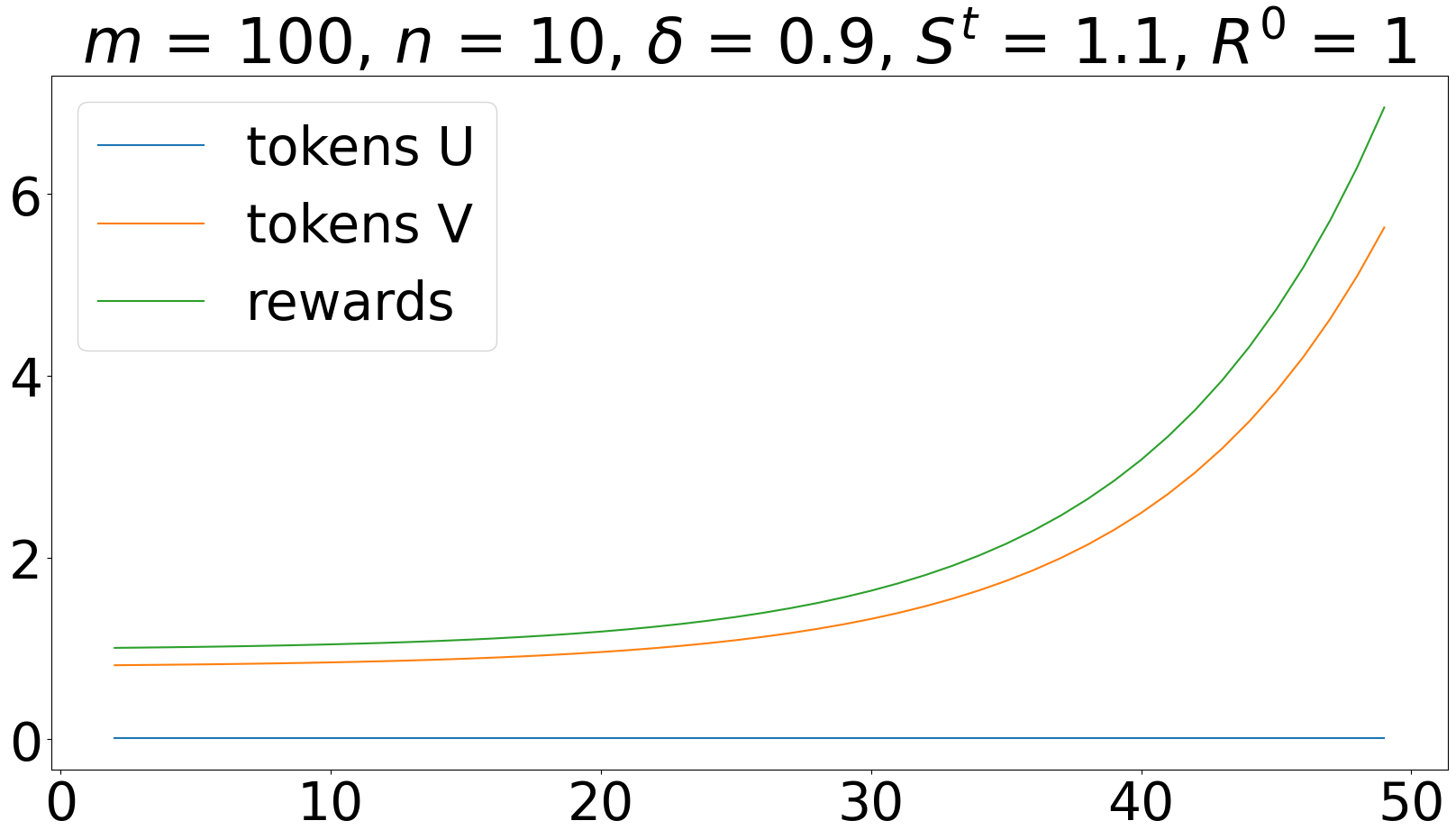
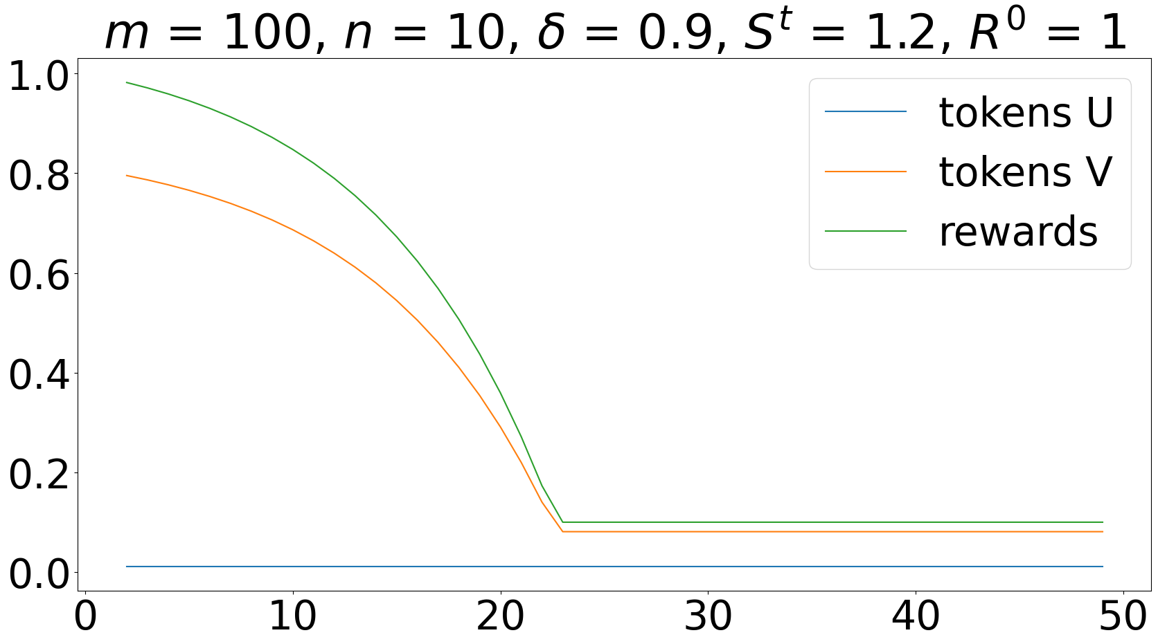
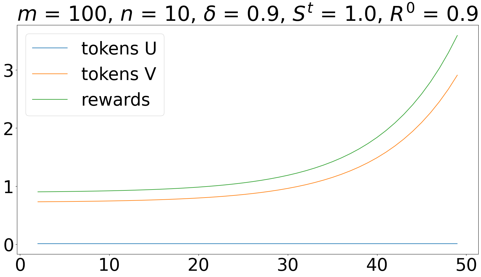
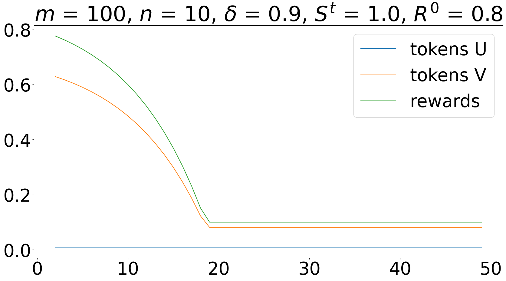
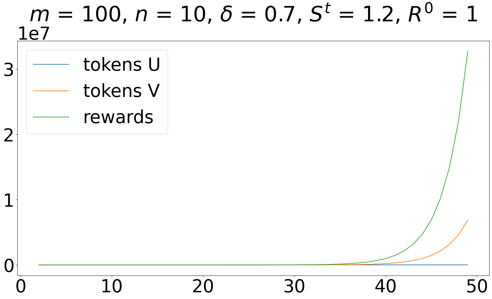
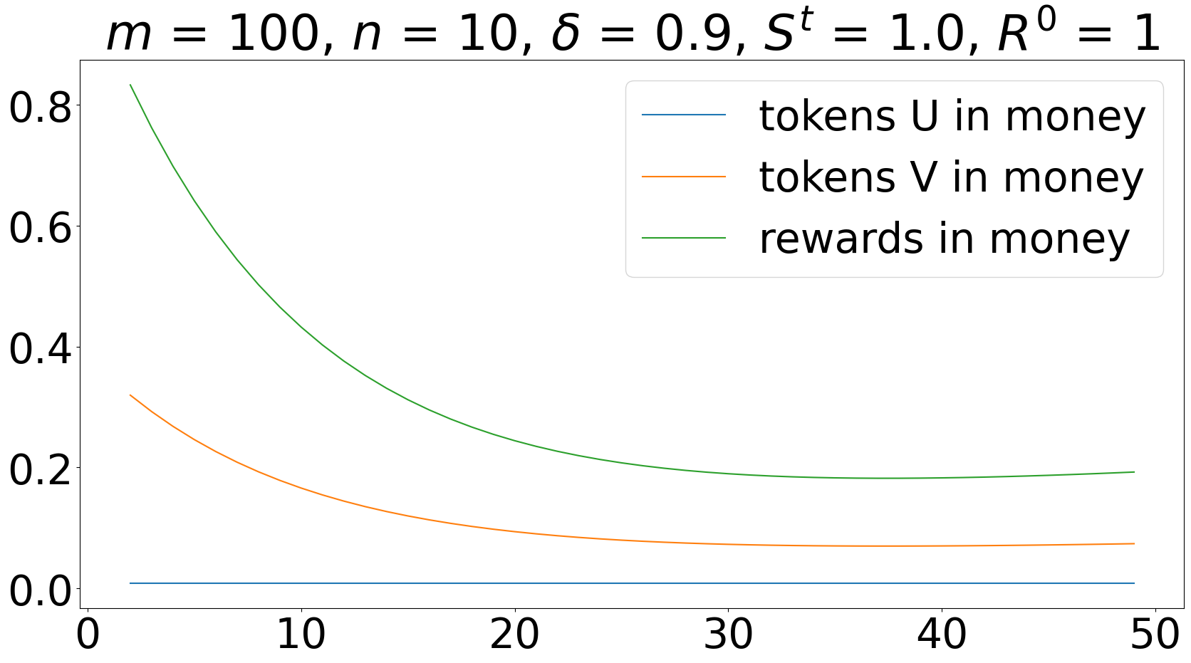
In the following experiment, we consider constant service value and rewards that are set to the minimal value necessary in order to have no buyback (Theorem 13), and also impose the rewards to not be below some minimum value (set to 0.1 for the sake of exposition). For the sake of simplicity, we consider the rewards and cost sharing schemes in (15) and , and observe the following:
-
Sufficiently high service value can avoid rewards explosion (Figure 2 compares two different service values under the same conditions). The necessary increase in the service value may simply be not possible due to inherent technological limitations and other external factors.
-
Sufficiently small initial rewards also avoid the rewards explosion (Figure 3 compares two initial rewards under the same conditions). Rewards however cannot be arbitrarily small since they must cover the costs of validators and be competitive against other sources of investments.
-
A higher risk free rate may also trigger an exponential growth (Figure 4 shows that for smaller we need a smaller initial reward, or a larger service value, to avoid this explosion).
-
Allowing the token price to decrease does avoid the rewards explosion that instead occur with stable prices, once we consider the rewards in money (Figure 5). Decreasing prices are however not desirable, and perhaps one may want increasing prices, which turn out to make the monetary reward explosion even more severe.
The above uncontrolled growth represents a potential “death spiral” stemming from necessary equilibrium conditions. First, it leads to impractical implementation due to numerical explosion in ledger validators accounts (thus violating feasibility). Second, it may even render such equilibria nonexistent for some parameter combinations. Note that adapting the rewards requires knowledge about shocks far in the future. Indeed, Theorem 13 states that rewards cannot be reduced arbitrarily from one step to the next. Such powerful oracles are generally not available, and solutions based on them also violate feasibility.


3.4 Policy that accommodates and implements the stable price equilibrium
In this section, we consider the fundamental question of how one can compute and implement an equilibrium with stable prices satisfying the no buyback condition. Stable prices require to keep a precise amount of tokens of users (on one side) and of tokens of validators (on the other side) given by Corollary 10. The no buyback condition requires the system to set the rewards so to satisfy the condition in Theorem 13. For the sake of exposition, we next describe an implementation for the reward and service fee schemes in (11). We should point out that this implementation does not specify how to set the initial rewards which is the crucial point to avoid rewards explosion (Corollary 14).
Given parameters and constraints.
-
1.
The risk free rate and thus the discount factor .
-
2.
The total number of users and the total number of validators (both constant over time).
-
3.
There is no need for the system to buyback tokens (Definition 12).
System parameters.
The system design depends on essentially two parameters:
-
1.
Total value of the service which is divided among the users at each step .
-
2.
Total amount of rewards which is distributed to the validators at each step .
Suggested equilibrium description and properties.
At each round ,
-
1.
Users strategies:
-
(a)
Start with tokens, where .
-
(b)
Spend all these tokens to get a service value equal to .
-
(c)
Given the next round service value , buy tokens required for the next round according to Item 1a.
-
(a)
-
2.
Validators strategies:
-
(a)
Start with tokens, where .
-
(b)
Stake all these tokens to get new tokens as reward.
-
(c)
Given the rewards of next round, sell this amount of tokens (if negative, buy tokens): , which yields the required tokens for next round according to Item 2a.
-
(a)
-
3.
System actions:
-
(a)
Given the next round service value , set the next total rewards so that
which guarantees the no buyback condition, that is, .
-
(b)
Announce the next rewards before the token buy or sell (Subround II) begins.
-
(c)
Sell the required amount of tokens, , to match demand during Subround II.
-
(a)
-
4.
Prices: all tokens are exchanged at a stable price .
4 A two-token model
In this section, we consider a natural variant of the previous (single-token) model to the case in which we have two tokens, token and , whose use and purpose is as follows:
-
token is used by the users to pay and get the service, and
-
token is used by the validators for staking to get rewarded with more tokens (of both types).
A number of existing systems follow a similar two-token scheme (see Figure 6 for some examples) and a model based on the similar assumptions has recently been proposed by [9]. Both tokens can be exchanged in the spot market as before, and thus we have a price for each token (see Figure 7 for some additional notation for the two-token model). The corresponding utilities are naturally given by
| (21) | |||||
| (22) |
| System | token | purpose | token | purpose |
|---|---|---|---|---|
| DFINITY ([27]) | ICP | staking & rewards | Cycle | computation (service) |
| NEO ([19]) | NEO | staking | GAS | pay transactions |
| Axie Infinity ([12]) | AXS | governance and staking | SLP | play (breeding Axie) |
| IOTA ([23]) | IOTA | staking & rewards | Mana | access ledger |
-
is the reward at time .
-
is the selling strategy of validator .
-
is the buying strategy of user .
-
is the amount of token used by user to pay for the service.
-
are the token holdings of a generic player (a user or a validator).
-
are the prices of the two tokens.
For the sake of exposition, we consider the simpler reward sharing and payment schemes (15), where token is used for staking, and each validator is rewarded with quantities and of tokens and , respectively. Users get a service value depending on the amount of tokens they use, i.e., they pay to the system. Thus, we have
| (23) |
The validators’ selling constraint for the single token (5) extends naturally into
| (24) | |||
| (25) |
Similarly, the users’ selling constraint for the single token (6) extends as follows:
| (26) | |||
| (27) |
where the asymmetry is due to the fact that only token is used for getting the service, by paying tokens. We next generalize the condition of (symmetric) equilibrium (Definition 1 and Remark 2) by requiring a “minimal” set of selling constraints to be non-strict (see Remark 18 below).
Definition 17 (symmetric equilibrium two tokens).
Consider a system policy given by (23), and a triple of users’ strategies, validators’ strategies, and prices, , such that the corresponding selling constraints of users (26)-(27) and of validators (24)-(25) are satisfied. We say that such a triple is an equilibrium if, for every user and every validator
-
1.
maximizes the discounted utility (21) of user , given all other strategies
-
2.
maximizes the discounted utility (22) of validator , given all other strategies
-
3.
the selling constraint of token are non-strict for user (resp., token for validator ), and thus the corresponding token holdings are strictly positive, that is, and
Moreover, we say that such an equilibrium is symmetric if the token holdings of all users are the same, and similarly, if all token holdings of all validators are the same. In particular, we have
| (28) |
for all users and for all validators and for all .
Remark 18 (minimal strict selling constraints).
Note that in the definition above, each type of player – validator or user – has non-strict selling constraint only in its own “main purpose” token (see Equation 28). This corresponds to the natural requirement of continuous participation in staking and in accessing and paying for the service. Furthermore, the price analysis below implies that equilibria with certain desired prices are impossible if some of the other selling constraints is also strict.
The next lemma is a generalization of [11, Lemma 1] to two tokens (see also [15] for details), and it provides conditions in the prices based on the validators’ strategies.
Lemma 19 (validators part).
In the two-token model, the corresponding prices in any symmetric equilibrium must satisfy the following conditions. If the selling constraints of are non-strict, then If the selling constraints of are non-strict, then
| (29) |
where
| (30) |
and is the token holding (staking) of any validator at this equilibrium.
Note that these two expressions in (30) are not symmetric in the two tokens, as the staking token appears in both denominators.
We next consider how the users’ buying strategies relate to the prices.
Lemma 20 (users part).
In the two-token model, the corresponding prices at any symmetric equilibrium must satisfy the following conditions. If the buying constraints of are non-strict, then
Moreover, if the selling constraints of are non-strict, then
4.1 Generic symmetric equilibria
The following class of generic equilibria captures equilibria in the two-token model where prices of token are -stable, that is, they satisfy (16), thus in particular the case in which we aim at stable prices for token used by the user to get the service.
Definition 21 (generic symmetric equilibrium for two tokens).
A symmetric equilibrium for the two token model is generic if the following conditions hold for all :
-
1.
The service to fees ratio is constant,
-
2.
The prices of satisfy
where constant depends only on the number of users , the number of validators , and on the service fee scheme.
-
3.
Each user starts round with the same token holding , uses all its current holding tokens for the service (), and buys new tokens needed for the next round accordingly ().
-
4.
For the following rewards to stake ratios, the prices of satisfy
(31) where constant depends only on the number of users , and on the rewards sharing scheme.
Theorem 22.
Proof.
4.2 No buyback in the two-token model
In this section, we study the implications of no buyback in the two-token model. As for the single token setting, we aim at equilibria where the system does not need to buyback tokens of either type.
Definition 23 (no buyback two tokens).
We say that a symmetric equilibrium in the two-token model satisfies the no buyback condition if no additional tokens (of either type) are bought at any round by the system, that is, and .
The following theorem provides a bound on the rewards that depends only on the next round’s service value. The main advantage of the two-token model is that rewards can be adjusted “immediately” to the service value fluctuations, and they need to be low only when the latter is low. The mechanism in Section 4.3 implements this idea.
Theorem 24.
In any generic symmetric equilibrium, there is a maximum monetary reward for validators in terms of tokens that can be awarded without violating the no buyback condition. In particular, it must hold
This is because validators always sell all the newly rewarded tokens and users buy (only) tokens of type , thus implying that validators keep all their tokens and possibly buy new ones, .
Proof.
We consider the two inequalities of the no buyback condition (Definition 23) separately.
-
1.
For tokens of type , we observe that, for , the users buying strategies satisfy Moreover, the validators’ selling strategies satisfy since the validators selling constraint for tokens of type must be strict, and thus for all . Therefore the no buyback condition for tokens of type is equivalent to
- 2.
This completes the proof.
4.3 Stable price mechanism in two-token model
We next describe a simple mechanism which implements stable prices for token , while the equilibrium price of token tends to grow but is affected by the shocks. The system provides rewards with tokens only. At equilibrium, validators keep their tokens as they guarantees access to rewards, and sell only tokens . More in detail:
-
1.
In order to have stable prices for and no buyback, we set such that , where is the constant given by Theorem 24 that makes the no buyback condition hold tightly. Furthermore, we set .
- 2.
-
3.
From the previous equation, the discounted utility of validators, if deviating by selling all tokens at some round , is at most while the discounted utility for the suggested strategies (equilibrium) equals
-
4.
In order to have feasible (nonnegative) prices, we need to set the initial payments and token holdings sufficiently high.
Theorem 25.
Proof.
We follow a similar argument as in [11, Remark 2 (existence)] based on the following three conditions. First, the discounted utilities of all players (users and validators) assume finite values (since their instantaneous utilities are proportional to ). Second, these strategies at equilibrium are in some bounded interval . For users, this is evident since they buy tokens proportionally to and from Assumption 1. For the validators, they sell all tokens , they never sell or buy tokens . Third, the utilities of the players are concave due to Assumption 2. Finally, Theorem 4.5 in [26] yields the desired result (concavity implies that the necessary equilibrium conditions maximize a round- decomposition of the utility (see full version [15]), while Theorem 4.5 in [26] ensures the maximum for the decomposition indeed maximizes the corresponding player utilities, thus an equilibrium).
4.3.1 Stable price mechanism implementation
At each round , the system only needs to estimate the next round service value , and thus a simpler “one step lookahead” oracle suffices, as opposed to the single-token case. Then, we have the following simple mechanism:
-
1.
Users use (spend) tokens proportionally to and buy new tokens proportionally to the next round service value .
-
2.
Validators’ rewards consist of only tokens proportionally to the next round service value .
-
3.
Validators sell all these tokens that they get as rewards, and keep all tokens they had from the beginning.
It is worth pointing out that in our two-token model, users can also buy tokens , and validators can sell them as well. However, in the equilibria induced by the proposed mechanisms, it is not convenient for either party to do so.
Remark 26.
We note that the equilibria described above are closely related to certain proposed implementations of IOTA ([23]). As in our proposed reward scheme and equilibria, rewards in the IOTA system are uniquely provided in the form of Mana tokens (= token ), while staking is conducted via IOTA tokens (= token ). Furthermore, only Mana tokens can be traded to “[…] individuals that in some sense are external to the system” [23]. In this context, our equilibria demonstrate that such designs, which forbid trading governance tokens, may still be sustainable. Specifically, Theorem 25 says that there exist equilibria where, even if trading governance tokens indirectly via some off-chain/secondary market became possible, players would not find it advantageous to do so.
5 Conclusions and research directions
We studied the problem of token monetary policy in blockchain systems viz-à-viz a set of desiderata that are crucial for the security and sustainability of blockchain systems. Our analysis lead to our proposal of a new general tool for tokenomics policy, quantitative rewarding, which judiciously adjusts the rewards given to validators with the objective of achieving, at equilibrium, desirable paths for the token price, e.g., stable prices. In the light of this, we investigated how the long-term equilibria between users, validators and token flows are different for blockchains with a single token (used for transaction fees and staking) and two separate tokens. An important finding of this analysis, is that the two-token model affords additional flexibility that can handle a broader variation of service values at equilibrium. Specifically, on the issue of implementation of monetary policies satisfying all our desiderata, the results for single token tokenomics in Section 3 highlight the need for some “global” information about future fluctuations in the service value, making such policies difficult to realize (namely, in order to avoid buybacks and price fluctuations, oracles that predict future shocks are needed to avoid reward explosion). In two-token systems, instead, the policy only needs to know the near future service value to control prices and enforce all our desiderata, a more tractable objective. In summary, in order to facilitate all our desiderata for a monetary policy, a suitable proxy for the service value is essential, and for two-token systems the presence of such proxy can be put to use much more effectively via our proposed QR mechanism. Future work could delve into assessing various possible proxies and their on-chain implementation as well as the incentive compatibility for users and validators that now will have the additional leverage of observing any of the oracle computations and data dependencies that may be taking place publicly on-chain and could be influenced by their actions.
References
- [1] Yannis Bakos and Hanna Halaburda. The role of cryptographic tokens and ICOs in fostering platform adoption. CESifo Working Paper, 2019. URL: https://ideas.repec.org/p/ces/ceswps/_7752.html.
- [2] Yannis Bakos and Hanna Halaburda. Overcoming the coordination problem in new marketplaces via cryptographic tokens. Information Systems Research, 33(4):1368–1385, 2022. doi:10.1287/ISRE.2022.1157.
- [3] Jeff Burdges, Alfonso Cevallos, Peter Czaban, Rob Habermeier, Syed Hosseini, Fabio Lama, Handan Kilinc Alper, Ximin Luo, Fatemeh Shirazi, Alistair Stewart, and Gavin Wood. Overview of polkadot and its design considerations, 2020. arXiv:2005.13456.
- [4] Tarun Chitra. Competitive Equilibria Between Staking and On-chain Lending. Cryptoeconomic Systems, 0(1), 2021. URL: https://cryptoeconomicsystems.pubpub.org/pub/chitra-staking-lending-equilibria.
- [5] Lin William Cong, Zhiheng He, and Ke Tang. The tokenomics of staking. Preprint, submitted April, 6, 2022.
- [6] Lin William Cong, Ye Li, and Neng Wang. Tokenomics: Dynamic adoption and valuation. The Review of Financial Studies, 34(3):1105–1155, 2021.
- [7] Lin William Cong, Ye Li, and Neng Wang. Token-based platform finance. Journal of Financial Economics, 144(3):972–991, 2022.
- [8] Cosmos SDK. Gas and Fees. {https://docs.cosmos.network/main/learn/beginner/gas-fees}.
- [9] Nicola Dimitri. The economic value of dual-token blockchains. Mathematics, 11(17):3757, 2023. doi:10.3390/math11173757.
- [10] Ester Félez-Viñas, Sean Foley, Jonathan R Karlsen, and Jiri Svec. Better than bitcoin? can cryptocurrencies beat inflation? Available at SSNR, 2021. URL: https://dx.doi.org/10.2139/ssrn.3970810.
- [11] Samuel Häfner. Optimal decentralization and service provision on a blockchain platform with market frictions, September 2023. URL: https://papers.ssrn.com/sol3/papers.cfm?abstract_id=3954773.
- [12] Axie Infinity. Axie infinity whitepaper, 2021. NEO & GAS. URL: https://whitepaper.axieinfinity.com/axs.
- [13] Urban J Jermann. A macro finance model for proof-of-stake ethereum. Available at SSRN 4335835, 2023.
- [14] Kose John, Thomas J Rivera, and Fahad Saleh. Equilibrium staking levels in a proof-of-stake blockchain. Available at SSRN, 3965599, 2021.
- [15] Aggelos Kiayias, Philip Lazos, and Paolo Penna. Single-token vs two-token blockchain tokenomics. arXiv preprint arXiv:2403.15429, 2024. doi:10.48550/arXiv.2403.15429.
- [16] Aggelos Kiayias, Philip Lazos, and Jan Christoph Schlegel. Would Friedman Burn your Tokens? Financial Cryptography and Data Security (FC 2024), 2024. Also available as arXiv preprint arXiv:2306.17025. doi:10.48550/arXiv.2306.17025.
- [17] Ricardo Lagos and Randall Wright. A unified framework for monetary theory and policy analysis. Journal of political Economy, 113(3):463–484, 2005.
- [18] Jiasun Li and William Mann. Digital tokens and platform building. The Review of Financial Studies, 38(7):1921–1954, 2025.
- [19] neo.org. NEO & GAS. URL: https://neo.org/neogas#tokens.
- [20] Christina Ovezik, Dimitris Karakostas, Mary Milad, Aggelos Kiayias, and Daniel W. Woods. Sok: Measuring blockchain decentralization, 2025. doi:10.48550/arXiv.2501.18279.
- [21] Emiliano S Pagnotta. Decentralizing money: Bitcoin prices and blockchain security. The Review of Financial Studies, 35(2):866–907, 2022.
- [22] Julien Prat, Vincent Danos, and Stefania Marcassa. Fundamental Pricing of Utility Tokens. Working Papers hal-03096267, HAL, 2021. URL: https://ideas.repec.org/p/hal/wpaper/hal-03096267.html.
- [23] Olivia Saa, Andrew Cullen, and Luigi Vigneri. Iota 2.0 incentives and tokenomics whitepaper, 2023. URL: https://www.iota.org/foundation/research-papers.
- [24] Fahad Saleh. Blockchain without waste: Proof-of-stake. The Review of financial studies, 34(3):1156–1190, 2021.
- [25] Linda Schilling and Harald Uhlig. Some simple bitcoin economics. Journal of Monetary Economics, 106:16–26, 2019.
- [26] N Stokey. Recursive Methods in Economic Dynamics. Harvard University Press, 1989.
- [27] The DFINITY Team. The internet computer for geeks. Cryptology ePrint Archive, Paper 2022/087, 2022. URL: https://eprint.iacr.org/2022/087.