PvpAMM: A Perpetual Market for Unbalanced Long-Short Positions

Abstract
Perpetual futures – swap contracts without expiration dates – are the most widely traded derivatives in cryptocurrency markets. Traditional perpetual trading relies on order books, which require substantial bilateral liquidity and face challenges in high-volatility environments. In this paper, we introduce pvpAMM, a peer-to-peer perpetual trading protocol based on automated market maker (AMM) principles. The protocol enables efficient settlement of long-short mismatched markets and drives positions toward equilibrium: when the minority leveraged side wins, their returns are amplified compared to conventional perpetual contracts, while the opposite occurs when the majority side prevails. We also propose arbitrage mechanisms to maintain economic equilibrium within the pvpAMM system. By incorporating liquidity providers (LPs), the protocol aligns more closely with traditional order book trading. Numerical experiments validate our theoretical findings.
Keywords and phrases:
Perpetuals, Decentralized Finance, Auto Market Making, BlockchainCopyright and License:
![[Uncaptioned image]](x1.png) © Zhenhang Shang, Zhenyu Zhao, and Kani Chen; licensed under Creative Commons License CC-BY 4.0
© Zhenhang Shang, Zhenyu Zhao, and Kani Chen; licensed under Creative Commons License CC-BY 4.0
2012 ACM Subject Classification:
Applied computing Digital cash ; Mathematics of computing Stochastic processesFunding:
We acknowledge the support from the Hong Kong RGC through GRF Grants 16310222, 16308221 and 16308421.Editors:
Zeta Avarikioti and Nicolas ChristinSeries and Publisher:
 Leibniz International Proceedings in Informatics, Schloss Dagstuhl – Leibniz-Zentrum für Informatik
1 Introduction
1.1 Background
Perpetual contracts have emerged as the cornerstone of cryptocurrency derivatives trading, enabling leveraged speculation and hedging without requiring holders to roll over the underlying asset. Dominating digital asset markets with daily volumes exceeding $100 billion, they surpass traditional futures in both liquidity and accessibility [3]. However, their unique structure – continuous funding payments, no expiration, and 24/7 settlement – introduces critical challenges for maintaining balanced markets during extreme volatility or unilateral trading pressure.
Traditional implementations rely on centralized limit order books (CLOBs), where execution requires matching long and short order volumes. While straightforward, this mechanism proves fragile in skewed markets: liquidity providers face asymmetric risks that widen spreads, increase fees, and may cause market failure [5]. The zero-sum nature of derivatives exacerbates these issues, as directional exposure imbalances cannot be resolved without substantial trader costs.
We present a paradigm-shifting solution through the first complete automated market maker (AMM) framework specifically engineered for perpetual futures, which systematically addresses the persistent position imbalance problem while simultaneously enhancing capital efficiency and trader profitability. Unlike traditional AMM designs originally conceived for prediction markets [6] or simple spot trading [9, 12], our protocol introduces leveraged, state-aware liquidity provisioning that dynamically adjusts pricing curves and exposure limits in response to real-time market conditions. This innovative approach enables the autonomous absorption of unilateral order flow without dependence on external arbitrageurs or centralized liquidity pools, representing a fundamental advancement in decentralized finance infrastructure. Our solution finally bridges the critical architectural gap that has forced perpetual contracts to remain tethered to centralized order book models despite their inherent incompatibility with DeFi’s core principles.
Our research makes three foundational contributions to decentralized derivatives markets:
-
A leveraged trading protocol resolving position imbalances, with profitability comparisons against traditional order books.
-
Novel arbitrage mechanisms that sustain economic equilibrium, detailing liquidity providers’ role in maintaining protocol stability.
-
Comprehensive agent-based simulations evaluating protocol efficacy through diverse participant interactions.
1.2 Related Work
Perpetual contracts were first suggested by Shiller in [24] as a means of hedging illiquid assets, and they later gained widespread popularity as a method for taking leveraged positions in cryptocurrency markets [11]. The existing literature on perpetual futures primarily focuses on descriptive evidence. For instance, Alexander et al. [3] found that BitMEX derivatives lead the price discovery process across major Bitcoin spot exchanges. Hung et al. [23] identified significant pricing effects and breakpoints in market efficiency. Additionally, some researchers have addressed the challenges of perpetual trading by proposing derivatives with alternative return structures. For example, D. White proposed a perpetual contract with returns proportional to some power of the spot price in [27], leading to the creation of a decentralized perpetual protocol on the Ethereum blockchain called Squeeth [21]. However, this protocol splits total liquidity and does not resolve the issue of unequal positions.
AMMs have been utilized in various applications within the DeFi ecosystem, primarily popularized by token swap protocols [2, 4, 13]. They have also been adapted for several DeFi applications, including crypto options (e.g., Hegic [28]), rate swaps (e.g., Voltz [16]), and NFT exchanges (e.g., Caviar [10]). There is emerging research on the economic implications of AMMs; however, much of it focuses on the incentives for liquidity provision, particularly the relationship between transaction fees and impermanent loss [15, 17, 8].
In the context of derivatives, a virtual AMM (vAMM) model has been implemented, which differs slightly from the conventional AMM. In a vAMM, there is no proper asset pool that supports the counterparty risk, resulting in under-collateralization. Due to this under-collateralization, many vAMMs maintain an insurance pool to cover potential losses. However, this can lead to adverse selection by traders when liquidations do not occur in a timely manner. Some researchers have even argued that perpetual contracts designed through vAMMs resemble a Ponzi scheme that cannot be sustained [2]. In [14], GMX X4 introduced a peer vs. peer (pvp) mechanism for executing perpetual contract transactions via AMMs. LionDex later referenced this design in [18], but their analysis was restricted to narrow use cases – primarily liquidity pool initialization and single-price updates, without accounting for multi-period price dynamics. Their model also suffers from mathematical inconsistencies, particularly in modeling the effect of leverage on returns (see Section 2.3 for a detailed critique).
2 Preliminaries
2.1 Notations
Let denote the spot price of the underlying asset at time . Contract positions are indexed by . For position , let denote its creation time and its clearing time, with the ordering assumed without loss of generality. The collateral for the position is , and the leverage is , where indicates a long position, a short position, and designates a liquidity provider(LP) role.
At time , the user borrows an amount to acquire units of the underlying asset. Ignoring liquidations, the conventional value of position at time , where , is given by:
Position will be liquidated if falls below a specified threshold. Specifically, the bust time for is defined as:
where denotes the infimum, and is typically set to 0. When the set is empty, we adopt the convention , which implies no liquidation occurs before . Let be the indicator function, with if is true and otherwise. The conventional value of the -th perpetual contract over is:
Note that depends only on and , so the process is adapted to the filtration generated by .
2.2 pvpAMM Dynamics
In an AMM-based protocol, a liquidity pool serves as the sole counterparty for each transaction, utilizing a conservation function to algorithmically price positions and restrict price movements to predefined trajectories [29]. A perpetual AMM protocol typically involves two types of interaction mechanisms: (1) the establishment, clearing, and liquidation of leveraged positions; (2) the provision and withdrawal of liquidity. These interactions must be specified in a way such that desired invariant properties are upheld.
To illustrate the problem addressed by the pvpAMM protocol, we consider the simplest scenario where all positions remain active post-creation. Similar analysis in more complex scenarios leads to analogous conclusions (see B.2). For time where:
the total assets in the liquidity pool are:
and the total value of all positions is:
The primary challenge for pvpAMM is to distribute the available collateral to individual position values when , preserving protocol solvency and economic incentives. A straightforward method is to distribute funds in proportion to their conventional worth:
Proposition 1.
if , reducing the incentive to create new positions.
Proposition 2.
if , leading to a flash-loan attack where an attacker profits by borrowing at and exiting immediately.
The proofs of these propositions (Appendix A.1) demonstrate the insufficiency of this natural approach.
2.3 GMX’s Solution
To rectify the cash-wealth imbalance, GMX introduced an intermediate token, LPT. Let represent the price of LPT, and the LPT balance for position at time . The protocol functions as follows:
-
Establishment: , effectively purchasing LPT with .
-
Price Updates: for , .
-
Liquidation: position is liquidated if at any time
-
Clearing: at , the position holder receives back.
Some specific numerical examples are given in B.1. Actually we have:
Proposition 3.
as the time interval for price updates .
The proof is provided in Appendix A.2. In DeFi implementations, spot prices update with each on-chain operation. Consequently, frequent operations compound leverage’s effect on LPT balances exponentially, resulting in exponential position value growth.
3 Mechanisms
In this section, we present the mathematical framework governing our pvpAMM protocol. We begin by defining the PLT token system and establishing the fundamental value conservation properties. The dynamics of leveraged positions are then analyzed, with particular attention to the evolution of the scaling parameter . Finally, we derive the stochastic differential equation for and examine its probabilistic characteristics. The results provide a complete specification of the core mechanisms of the protocol.
3.1 PLT Token
The defining idea of our pvpAMM is “concentrated collateral and proportional worth": all collateral and worth for leveraged positions is pooled together, and the actual worth of each contract is realized in proportion to its conventional value. We incorporate a strategy from the GMX model, where is divided by the current (cash)/(position value) scaling factor upon entering the pool. For better understanding, we introduce an intermediate token named PLT(PvpAMM Liquidity Token), priced at . When a position is established, an amount of PLT is recorded. As time progresses, the position’s PLT balance is adjusted to at time , and its value in the pvpAMM pool is calculated as:
The price of PLT, , is determined by the ratio of total collateral to total PLT balance:
measures the amount of numéraire that the -th contract can retrieve if cleared at time . The PLT price acts as a normalization factor, ensuring that the total value of all contracts equals the remaining cash amount, the conservation function for our pvpAMM protocol can be written as:
The PLT mechanism operates similarly to a casino’s chip system. Just as a casino maintains a fixed cash reserve backing all chips in circulation, the protocol pools all collateral to back PLT tokens. When traders open positions, their collateral converts to PLTs at the current exchange rate, much like purchasing casino chips with cash. The PLT price fluctuates based on the aggregate performance of all open positions - when collective gains exceed losses, the PLT appreciates, and vice versa. Traders closing positions redeem their PLTs at the prevailing rate, ensuring the system remains fully collateralized at all times. This creates a self-balancing ecosystem where value flows naturally between participants while maintaining systemic solvency.
For computational convenience, we set , and get:
Proposition 4.
The scaler function satisfies:
By setting the initial value , we have one definite and unique solution for . It is continuous, and unless no live contracts exist at time t.
Proof.
The expression for can be derived directly from equation (1). We assume at any time there is at least one contract live, this can be easily satisfied by setting up a long contract at time 0 with leverage , which will never bust. From (2) we know is left-continuous. Since is continuous for , it is seen from (2) that is continous over that is not the event times
For the position creation time , we may find that
the continuity of is thus proved.
To show with at least one live contract at time , we define , with the convention of , then for all . If is finite, the numerator in (2) will converge to 0 as . This implies there are live contracts right before , and they all bust at , which cannot happen as we assumed there is always one live contract at any time.
Note that the calculation of in (2) only involves for , indicating an iterative algorithm for computing . We can iteratively determine based on all previously computed values of at the event times that occur before . Additionally, if there are no events for establishing or clearing positions in the time interval , the sets and are identical. Under this condition, we have:
with the continuity of , this formula may be used to efficiently compute .
3.2 Leveraged Positions
In this section, we clarify the state transitions of the defined pvpAMM market when operating with leveraged positions. Consider two trading positions, for Alice and for Bob. To demonstrate the system’s behavior across different stages, we specifically consider a scenario where . The trading activities in our protocol function as follows:
-
Initialization. we initialize for .
-
Establishment. for ,
Alice can close her position at any time during this period to reclaim her collateral , it occurs without any profit or loss, as there is no counterparty involved.
For :
where and represent the amounts each position would receive if closed at time ,
-
Clearing. Alice closed her position at time , withdrew from the pool. for :
The above discussion illustrates how is updated and its role in the trading process. For any leveraged position, the presence of a counterparty is not strictly necessary. Even with only positions in the same direction, such as all long positions, trading can still proceed. In this case, the less leveraged positions effectively act as short positions(“relatively short”).
Numerical examples can be found in Appendix B.2.
3.3 Pricing Equation
For the interval , we have:
This suggests that, from the traders’ perspective, the ratio determines whether their profit(or loss) is greater or less than those in a conventional perpetual setup.
For notational simplicity, let
Observe that is left-continuous, it represents the balance of long and short positions in the pool: . means that the weighted long shares, adjusted by , are heavier than the weighted short shares, and vice versus.
Theorem 5.
The scalar function satisfies the stochastic differential equation:
Suppose the price process satisfies
with a standard Brownian motion, and , continuous functions. If , namely, the price process is a martingale, then is a positive martingale. In this case, for all , and converges almost surely as .
Proof.
Equation (5) directly follows from differentiating both sides of equation (2). If follows geometric Brownian motion, we have
when , , is a local martingale, given that is positive, it is also a true martingale by the positive martingale property [19]. Then, , is bounded in expectation. By the Martingale Convergence Theorem, converges almost surely to some limit as .
Suppose , i.e. the weighted long positions are heavier than short positions, as seen from an interpretation of equation (5), increases (or decreases) along with the increase (or decrease) of . If , increases, and all long positions, the majority of the pool, get their profit from the difference . Note that the increase in suggests a diminished return compared to the conventional perpetual. Specifically, if Alice establishes the same position in a conventional setup and Bob does so in our protocol, Bob’s instantaneous return will be lower than Alice’s.
Conversely, if the pool (majority) is incorrect and decreases, also decreases. The decrease in implies a better return compared with a conventional perpetual. The same interpretation holds for the case where .
In summary, our protocol favors the overall performance of the pool. If the pool is correct, the established contracts yield worse returns than those in conventional perpetuals. If the pool is incorrect, the contracts yield better returns. For an individual position, the best return occurs when its direction is correct while the pool is wrong, whereas the worst return happens when the individual contract direction is incorrect but the pool is right.
4 Security Analysis
Security is paramount in DeFi protocols, particularly for innovative systems like pvpAMM. This section examines the security of our protocol from four aspects: (1) arbitrage maintains market equilibrium through price-stabilizing flows, (2) liquidity providers ensure stability via deposit/withdrawal dynamics, (3) flash loan resistance emerges from bounded profit potential, and (4) oracle reliability depends on feed accuracy and update frequency. These properties collectively ensure robustness against smart contract exploits, strategic manipulations, and data integrity threats.
4.1 Arbitrage Mechanisms for System Balance
In traditional perpetual contract trading markets such as centralized exchanges, prices of perpetual contracts are determined by secondary market transactions, and quantitative analysis between the spot and perpetual markets can identify arbitrage-free prices [1]. In contrast, our pvpAMM model determines the value of a position primarily through the price of PLT, denoted as . This value influences the strategies for position entry and exit, and arbitrageurs effectively trade over. Unlike in CEX, in pvpAMM is unaffected by secondary market transactions or market tendencies towards long or short positions; the determination of follows exclusively from the stochastic differential equation defined in Section 5. The pvpAMM protocol introduces an arbitrage mechanism that attracts minority orders, automatically balancing the long-short ratio by driving , as defined in 3.3, toward zero.
Theorem 6.
Arbitrage opportunities exist when .
Proof.
For simplicity, assume , and let , where is small. At time , user borrows dollars to: (1) purchase spot assets, (2) use dollar as collateral to open a position in the conventional market with leverage , and (3) use another 1 dollar as collateral to open a position in our pvpAMM with leverage . The arbitrage behavior here occurs in a short period of time, so the funding fee in the conventional perpetual market is negligible. The portfolio consists of the following four components:
-
Conventional perpetuals:
-
pvpAMM perpetuals:
-
Spot:
-
Cash:
From (5) and , we have:
The complete derivation appears in Appendix A.4. Note that , and the portfolio value at time is given by:
The portfolio is positive when arbitrageur set:
When , open a position with leverage implies relatively short position in pvpAMM, thereby driving downward. Vice versa when , open a position with leverage implies relatively long position in pvpAMM, thereby driving upward. The arbitrage opportunities exist when .
4.2 Liquidity Provision and Market Stability
Liquidity provision is a key mechanism for enhancing stability in decentralized finance (DeFi) systems – a critical factor in ensuring protocol security. In pvpAMM, liquidity providers act as counterweights to dominant pool positions, mirroring the stabilizing role of market makers in traditional perpetual markets.
By letting for the -th contract, we get a liquidity position:
this position will profit from a decrease in . Under the condition that , a decline in indicates a fall in , meaning the liquidity position is opposite to the direction of the majority of the pool’s positions. This is precisely the role of the LP, as it partially acts as a counterparty to the pool majority. Let , i.e. the first position be an LP position, actually, we may regard the first LP position establishment point as the process origin. We have:
Theorem 7.
Liquidity position makes the worth of our pvpAMM position closer to a conventional perpetual. Specially,
Proof.
for ,
then
Generally, traders interacting with the pool for leveraged positions have to reimburse LPs for supplying assets and living with the volitality of . This compensation comes in the form of swap fees that are charged on each position, and then distributed to liquidity pool shareholders [20]. Let be a small percentage of the trading fee, the pvpAMM protocol with fees is designed as follows:
4.3 Resistance to Flash Loan Attacks
Flash loan attacks – a prevalent threat in DeFi, as outlined in Proposition 2 – leverage rapid, uncollateralized borrowing to artificially distort market conditions. While earlier pvpAMM iterations were susceptible to such exploits, our protocol eliminates this vulnerability by preventing unanticipated profits from immediate position entry and exit, as formalized below.
Theorem 8.
The proposed pvpAMM protocol as 3.1 is resistant to flash loan attacks, i.e., there is no unanticipated profit from an immediate exit after entry.
Proof.
This follows directly from the continuity of 4: , thus
4.4 Oracle Price Feed Security
In decentralized finance (DeFi), accurate and timely price updates are critical to the functionality of the protocol, particularly for perpetual decentralized exchanges such as GMX and Jupiter. These platforms depend on oracles to provide asset price data, which underpins position valuation and overall protocol stability. However, oracles introduce potential attack vectors, including off-chain data manipulation, update latency, and centralization risks, all of which may compromise system integrity [26].
To mitigate these risks, modern DeFi protocols employ advanced oracle mechanisms. For example, Jupiter Perp integrates the Signal Oracle, a collaborative solution with Jupiter that enables compute-efficient multi-asset price updates in a single transaction, ensuring low latency and high reliability. Additionally, it supplements security with the Pyth Oracle for redundancy [25].
Decentralized oracle networks like Chainlink further enhance robustness by aggregating data from multiple sources, reducing manipulation risks. These systems use cryptographic attestations to verify data providers and employ aggregation methods to derive consensus prices – often accompanied by confidence intervals to indicate reliability [7].
5 Simulation
To validate the properties of our proposed pvpAMM protocol, we conducted numerical simulations. These simulations define a simulated underlying price process and explore how different types of agents interact with the protocol. The simulation runs for a predetermined number of time steps, updating prices and evaluating policies for introducing new agents at each step.
5.1 Market and Agents
The underlying market price is updated at each time step (after all agents have completed their actions) using the formula:
where is drawn from a normal distribution, and represent the mean returns and market volatility. In our simulation, we set and . The initial price is set to , with the timestep defined as .
We analyze the performance of positions in a simple market with three different types of users, where the leverage factor and the collateral are defined as in Section 2.1. The users and their default values are set to be:
-
Alice, who joins at , uses no leverage, i.e. , with a collateral.
-
Bob, who joins at , uses leverage long, i.e. , with a collateral.
-
Chris, who joins at , uses leverage short, i.e. , with a collateral.
5.2 Results

To investigate the property of , multiple experiments with different price series are conducted, we calculate and take their mean as our final value. The results, shown in Figure 1, indicate that consistently fluctuates around its expected value of 1.0, with lower volatility compared to .
The unique properties of our proposed pvp model under various market conditions are experimentally verified as follows:
5.2.1 No Counterparty Needed
Extreme market conditions often exhibit a clear one-sided sentiment, such as a bull market where all participants expect prices to rise, or a bear market where everyone anticipates a decline. In such scenarios, market makers are not necessary in our model to allow trader activities. For instance, in a bullish market where all traders anticipate an upward movement, their expectation of rising prices is reflected in the leverage of their trades: the stronger their belief in the price increase, the higher their leverage will be.
For example, if Bob takes a long position, while Chris opts for a long position, both entering at with collateral amounts of . Results shown in Figure 2(a) indicate that when the price rises, Bob achieves a positive return while Chris incurs a loss. Conversely, if the price drops – indicating a misjudgment by all traders, the outcomes reverse. Despite both being long positions, Chris is effectively at a disadvantage compared to Bob, whose smaller position yields returns akin to being short.
To further illustrate the impact of leverage, we conducted additional experiments where , and , ensuring that . Even under these conditions, Bob’s position beats Chris’s when the market price increases, and vice versa when price drops, see 2(b). This reinforces the conclusion that leverage is the critical factor: for long positions, less leveraged traders effectively act as relative short against more leveraged traders. A similar conclusion applies to short positions.
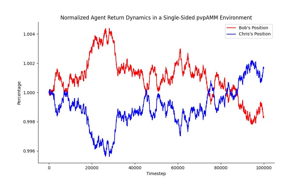
positions.
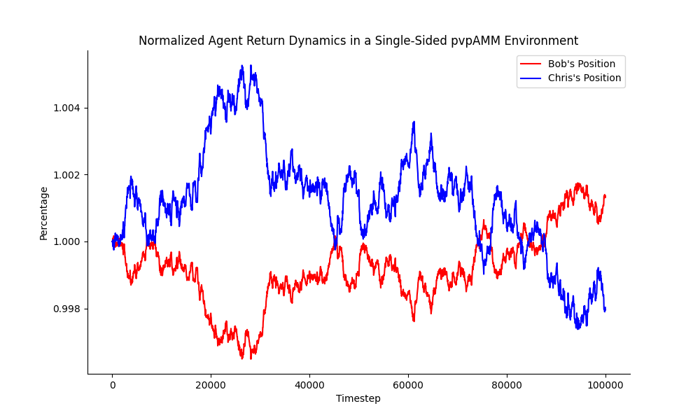
different leverage.
5.2.2 Auto Rebalancing in Unbalanced Positions
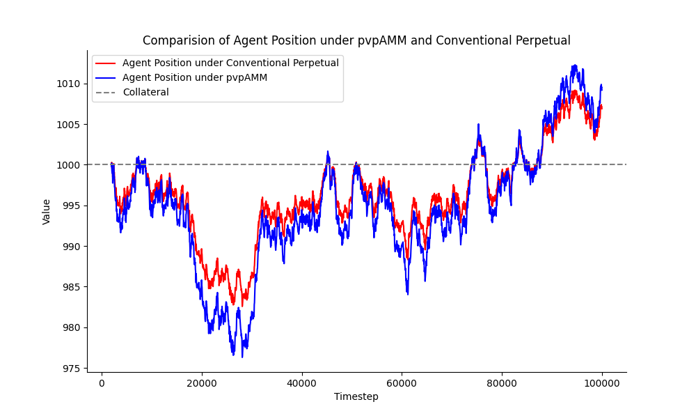
In a normal market where users hold differing directional views, the pvp protocol naturally encourages a balance between the long and short sides through economic incentives. It offers higher returns for the minority side while providing the majority side with lower but more stable returns. Figure 3 illustrates the dynamics of agent positions in this context. Bob, representing the minority, achieves a return that exceeds the conventional return when the price series trends upwards. Conversely, Chris, as the majority, incurs a negative return, however, this loss is less severe than what would be experienced in a conventional perpetual market.

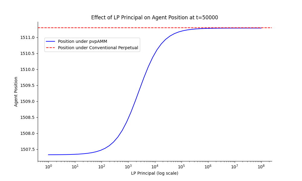
For liquidity providers in the protocol, Figure 4 illustrates the impact of the LP’s principal on at . As the LP position increases, Bob’s returns in the pvp protocol, , gradually converge to those of the traditional perpetual contract . This observation aligns with our derivations presented in 7.
6 Conclusion
We have detailed the design and implementation of pvpAMM, a peer-to-peer automated market maker (AMM) for perpetual contract transactions. The system proves particularly effective in markets with asymmetrical long and short positions, enabling a robust secondary market without traditional market makers or liquidity providers. The elimination of liquidity providers allows pvpAMM to extend derivative trading into smaller or markedly skewed market conditions, offering customized trading opportunities. Additionally, pvpAMM applies to prediction markets, where it can utilize trading behaviors to extract price insights and forecasts.
In deploying pvpAMM via blockchain smart contracts, careful attention is required for price determination to ensure the smooth handling of leveraged positions. The industry often adopts a multi-source oracle strategy to ensure reliability and accuracy, as elaborated in [30]. We include Solidity-based code for the critical modules of pvpAMM here, such as position opening, closing, and liquidation, to serve as a practical reference for readers [22].
Perpetual contracts are pivotal in finance, particularly within the cryptocurrency sector, where they traditionally depend on order books or liquidity pools with liquidity providers as counterparties. Our pvpAMM design addresses this reliance by introducing a new asset type, PLT. Analyzing PLT’s behavior under various spot price processes are left as future work.
References
- [1] Damien Ackerer, Julien Hugonnier, and Urban Jermann. Perpetual futures pricing. Technical report, National Bureau of Economic Research, 2024.
- [2] Hayden Adams and Noah Zinsmeister. Moody salem moody, uniswaporg river keefer, and dan robinson. uniswap v3 core. Technical report, Uniswap Foundation, 2021.
- [3] Carol Alexander, Jaehyuk Choi, Heungju Park, and Sungbin Sohn. Bitmex bitcoin derivatives: Price discovery, informational efficiency, and hedging effectiveness. Journal of Futures Markets, 40(1):23–43, 2020.
- [4] Guillermo Angeris and Tarun Chitra. Improved price oracles: Constant function market makers. In Proceedings of the 2nd ACM Conference on Advances in Financial Technologies, pages 80–91, 2020. doi:10.1145/3419614.3423251.
- [5] Guillermo Angeris, Tarun Chitra, Alex Evans, and Matthew Lorig. A primer on perpetuals. SIAM Journal on Financial Mathematics, 14(1):SC17–SC30, 2023.
- [6] Dmitriy Berenzon. Constant function market makers: Defi’s “zero to one” innovation. URL: https://medium.com/bollinger-investment-group/constant-function-market-makersdefis-zero-to-one-innovation-968f77022159, 2020. Accessed: 2025-08-08.
- [7] Lorenz Breidenbach, Christian Cachin, Benedict Chan, Alex Coventry, Steve Ellis, Ari Juels, Farinaz Koushanfar, Andrew Miller, Brendan Magauran, Daniel Moroz, Sergey Nazarov, Alexandru Topliceanu, Florian Tramèr, and Fan Zhang. Chainlink 2.0: Next steps in the evolution of decentralized oracle networks, 2021. URL: https://research.chain.link/whitepaper-v2.pdf.
- [8] Agostino Capponi and Ruizhe Jia. The adoption of blockchain-based decentralized exchanges. arXiv preprint arXiv:2103.08842, 2021.
- [9] Athos VC Carvalho, Douglas Silveira, Regis A Ely, and Daniel O Cajueiro. A logarithmic market scoring rule agent-based model to evaluate prediction markets. Journal of Evolutionary Economics, 33(4):1303–1343, 2023.
- [10] Caviar. Caviar. https://www.caviar.sh/, 2023. Accessed: 2025-08-08.
- [11] CoinGecko. Cryptocurrency derivatives (perpetual contract) by volume. https://assets.coingecko.com/reports/2022/CoinGecko-2022-Annual-Crypto-Industry-Report.pdf, 2022. Annual Crypto Industry Report. Accessed: 2025-08-08.
- [12] Richard Dewey and Craig Newbold. The pricing and hedging of constant function market makers. arXiv preprint arXiv:2306.11580, 2023. doi:10.48550/arXiv.2306.11580.
- [13] Michael Egorov. Stableswap-efficient mechanism for stablecoin liquidity. Retrieved Feb, 24:2021, 2019.
- [14] GMX. Gmx. https://gmxio.substack.com/p/x4-protocol-controlled-exchange, 2022. Accessed: 2025-08-08.
- [15] Joel Hasbrouck, Thomas J Rivera, and Fahad Saleh. An economic model of a decentralized exchange with concentrated liquidity. Available at SSRN 4529513, 2023.
- [16] Simon Jones and Artur Begyan. Voltz v2: A non-custodial clearinghouse. Technical report, Voltz, April 2023. Working Draft. URL: https://assets.website-files.com/61389177f5eab433827f7185/64353ecfebb1137bea5355d7_Voltz_v2_11Apr23.pdf.
- [17] Alfred Lehar and Christine A Parlour. Decentralized exchange: The uniswap automated market maker. Available at SSRN 3905316, 2021.
- [18] LionDEX. Liondex. https://liondex-official.gitbook.io/liondex/pvp-amm-protocol, 2023. Accessed: 2025-08-08.
- [19] Aleksandar Mijatović and Mikhail Urusov. On the martingale property of certain local martingales. Probability Theory and Related Fields, 152(1):1–30, 2012.
- [20] Allan Niemerg, Dan Robinson, and Lev Livnev. Yieldspace: An automated liquidity provider for fixed yield tokens. Retrieved Feb, 24:2021, 2020.
- [21] Opyn. Squeeth. https://squeeth.opyn.co/, 2021. Accessed: 2025-08-08.
- [22] pvpAMM. pvpamm codes. https://github.com/zhshang1221/pvpAMM, 2025. Accessed: 2025-08-08.
- [23] Qihong Ruan and Artem Streltsov. Perpetual contracts and market quality: Evidence from cryptocurrencies. https://papers.ssrn.com/sol3/papers.cfm?abstract_id=4218907, 2025. SSRN working paper. Originally posted: Sep 25, 2022. Last revised: Jun 22, 2025. Accessed: Aug 8, 2025. doi:10.2139/ssrn.4218907.
- [24] Robert J Shiller. Measuring asset values for cash settlement in derivative markets: hedonic repeated measures indices and perpetual futures. The Journal of Finance, 48(3):911–931, 1993.
- [25] Jupiter Team. Understanding how jupiter perps works: Complete guide, 2023. URL: https://station.jup.ag/guides/perpetual-exchange/how-it-works.
- [26] Sergey Tikhomirov, Pedro Moreno-Sanchez, and Matteo Maffei. Oracles in decentralized finance: Attack costs, profits and mitigation measures. Entropy, 25(1):60, 2023. doi:10.3390/E25010060.
- [27] D White, D Robinson, Z Koticha, A Leone, A Gauba, and A Krishnan. Power perpetuals, 2021.
- [28] Molly Wintermute. Hegic: On-chain options trading protocol on ethereum powered by hedge contracts and liquidity pools. Technical report, Hegic Protocol (via GitHub), February 2020.
- [29] Jiahua Xu, Krzysztof Paruch, Simon Cousaert, and Yebo Feng. Sok: Decentralized exchanges (dex) with automated market maker (amm) protocols. ACM Computing Surveys, 55(11):1–50, 2023. doi:10.1145/3570639.
- [30] Liyi Zhou, Xihan Xiong, Jens Ernstberger, Stefanos Chaliasos, Zhipeng Wang, Ye Wang, Kaihua Qin, Roger Wattenhofer, Dawn Song, and Arthur Gervais. Sok: Decentralized finance (defi) attacks. In 2023 IEEE Symposium on Security and Privacy (SP), pages 2444–2461. IEEE, 2023. doi:10.1109/SP46215.2023.10179435.
Appendix A Proofs
A.1 Proofs for Natural Worth Allocation in pvpAMM
We provide proofs for propositions within Section 2.2, which demonstrate that the natural worth allocation leads to disincentives for creating new positions when or vulnerabilities to flash-loan attacks when .
Proof.
A.2 Proof for LPT Balance in GMX’s Solution
We prove Proposition 3, which states that the LPT balance for position in the GMX protocol converges to
as the time interval for price updates .
Proof.
The price of LPT remains consistent across all positions and follows the equation:
then
A.3 Conservation and Continuity in pvpAMM with Position Clearing
In Section 3.1, we derived the conservation function and the scaler function for the pvpAMM protocol assuming all positions remain active after creation (see Proposition 4). Here, we extend the analysis to include position clearing at times , showing that the conservation function holds and that remains continuous at position creation () and clearing () times.
Conservation Function
and
Continuity of
Proof.
For the position creation time , we may find that
and for the clearing time , we have:
A.4 Derivation of Dynamics for Theorem 6
We provide the detailed derivation for the expression of used in the proof of Theorem 6.
Proof.
| (1) | ||||
Appendix B Numerical Examples
B.1 GMX’s LPT Solution
Use USD as the default numéraire. At time , Alice places a long order with 200 USD, leverage. Bob places a short order with 100 USD, leverage.
-
1.
, the initial spot price =100, the initial LPT price .
-
Alice’s LPT amount, .
-
Bob’s LPT amount, .
-
Total collateral is .
-
Total LPT amount is .
-
New LPT price .
-
Alice’s position value .
-
Bob’s position value .
-
-
2.
, assume the spot price rises 10% to .
-
Alice’s LPT amount, .
-
Bob’s LPT amount, .
-
Total collateral is .
-
Total LPT amount is .
-
New LPT price .
-
Alice’s position value .
-
Bob’s position value .
-
-
3.
, assume the spot price rises 10% to .
-
Alice’s LPT amount, .
-
Bob’s LPT amount, .
-
Total collateral is .
-
Total LPT amount is .
-
New LPT price .
-
Alice’s position value .
-
Bob’s position value .
-
B.2 pvpAMM’s PLT Solution
Use USD as the default numéraire. At time , Alice places a long order with 200 USD, leverage. Bob places a short order with 100 USD, leverage.
-
1.
, the initial spot price =100, the initial PLT price .
-
Alice’s PLT amount, .
-
Bob’s PLT amount, .
-
Total collateral is .
-
Total PLT amount is .
-
New PLT price .
-
Alice’s position value .
-
Bob’s position value .
-
-
2.
, assume the spot price rises 10% to .
-
Alice’s PLT amount, .
-
Bob’s PLT amount, .
-
Total collateral is .
-
Total PLT amount is .
-
New PLT price .
-
Alice’s position value .
-
Bob’s position value .
-
-
3.
, assume the spot price rises 10% to .
-
Alice’s PLT amount, .
-
Bob’s PLT amount, .
-
Total collateral is .
-
Total PLT amount is .
-
New PLT price .
-
Alice’s position value .
-
Bob’s position value .
-
B.3 LONG positions only in pvpAMM
Use USD as the default numéraire. At time , Alice places a long order with 200 USD, leverage. Bob places a long order with 100 USD, leverage.
-
1.
, the initial spot price =100, the initial PLT price .
-
Alice’s PLT amount, .
-
Bob’s PLT amount, .
-
Total collateral is .
-
Total PLT amount is .
-
New PLT price .
-
Alice’s position value .
-
Bob’s position value .
-
-
2.
, assume the spot price rises 10% to .
-
Alice’s PLT amount, .
-
Bob’s PLT amount, .
-
Total collateral is .
-
Total PLT amount is .
-
New PLT price .
-
Alice’s position value .
-
Bob’s position value .
-
-
3.
, assume the spot price rises 10% to .
-
Alice’s PLT amount, .
-
Bob’s PLT amount, .
-
Total collateral is .
-
Total PLT amount is .
-
New PLT price .
-
Alice’s position value .
-
Bob’s position value .
-