Heuristics for Covering the Timeline in Temporal Graphs

Abstract
We consider a variant of the Vertex Cover problem on temporal graphs, called Minimum Timeline Cover (-MinTimelineCover). Temporal graphs are used to model complex systems, describing how edges (relations) change in a discrete time domain. The -MinTimelineCover problem has been introduced in complex data summarization and synthesis jobs. Given a temporal graph , -MinTimelineCover asks to define activity intervals for each vertex, such that each temporal edge is covered by at least one active interval. The objective function is the minimization of the sum of interval lengths. -MinTimelineCover is NP-hard and even hard to approximate within any factor for . While the literature has mainly focused on the cases , in this contribution we consider the case . We first present an ILP formulation that is able to solve the problem on moderate size instances. Then we develop an efficient heuristic, based on local search which is built on top of the solution of an existing literature method.
Finally, we present an experimental evaluation of our algorithms on synthetic data sets, that shows in particular that our heuristic has a consistent improvement on the state-of-the art method.
Keywords and phrases:
Temporal Networks, Activity Timeline, Vertex Cover, Heuristic, Dynamic ProgrammingCopyright and License:
2012 ACM Subject Classification:
Mathematics of computing Graph algorithms ; Theory of computation Design and analysis of algorithms ; Theory of computation Mathematical optimization ; Theory of computation Discrete optimizationEditors:
Thierry Vidal and Przemysław Andrzej WałęgaSeries and Publisher:
1 Introduction
Complex systems are usually modeled through graphs or networks in order to understand their properties and behaviors. The availability of temporal information of relations between vertices has led to the introduction of temporal graphs [7, 13, 9], where edges, called temporal edges, represent interactions between two entities at a given time. Note that different variations of the temporal graph model have been introduced; here we consider a model where the time domain, over which the temporal edges are defined, is discrete [7, 13, 9].
Temporal graphs have been considered in several domains, e.g., social network analysis [17], computational biology [8] and epidemiology [1]. We consider an approach defined for the summarizations of temporal interactions in social networks [12, 16, 15, 14]. In this context, a user activity in a social network (called activity timeline) is represented with one or more time intervals; the goal is to represent users interaction, so that if an interaction is observed at time , then at least one of the user activity timeline include [14, 15, 6, 3, 2, 4, 5]. The objective function, following a parsimonious approach, is the minimization of the overall length (called span) of timeline activities or the minimization of the maximum length of the timeline activity. Here, we focus on the first objective function.
We present an example to show how activity timelines can be useful in understanding evolution of events. Consider the King Charles Coronation in May 2023. Figure 1 shows temporal co-occurrence of hashtag related to this event. The timelines, associated indicated in pink, helps to identify the main topics in the online discussions.
Several papers have studied the complexity of -MinTimelineCover [15, 6, 3, 2], also in some restricted variant. In particular, the case , where the activity timeline of each vertex is defined as a single interval, has been deeply studied, due also to the link with a foundational problem in theoretical computer science, that is Minimum Vertex Cover. For -MinTimelineCover is NP-hard and hard to approximate within constant factor [15, 6, 3, 2]. For , the problem is even harder, as even deciding if there exists a solution (of any span) is an NP-complete problem [15].
Due to the hardness of the problem and of its restrictions, some heuristic methods have been developed, for the general problem [15, 14] and for the restriction with [15, 14, 11]. Only the paper that has introduced -MinTimelineCover has designed practical methods for the problem [15] when , thus in this contribution we focus on designing methods for it. First, we design an ILP method that is able to solve the problem for moderate size instances, then we present a polynomial-time heuristic for -MinTimelineCover, based on local search, so that it is applicable even on larger temporal graphs. In order to design our heuristic, we present a dynamic programming algorithm for a related problem, called -MinIntervalCover, that runs in polynomial time.
We consider the performance of our methods on synthetic datasets, both in for the efficiency and the quality of the solutions returned. For this latter aspect we show that our heuristic, is able to shrink significantly the activity timeline lengths, with respect to the methods presented in [15].
1.1 Related Works
The complexity of -MinTimelineCover, including the parameterized and approximation complexity, has been considerably investigated. -MinTimelineCover is NP-hard, even for many restrictions. Rozenstein et al. have shown that it is NP-complete to decide whether the exists a solution of any span [15]; this implies that is not possible to approximate the problem within any factor. Also for it is NP-complete to decide whether there exists a solution of -MinTimelineCover that has span equal to [6].
The case is known NP-hard also when temporal graphs have some restrictions: at most one temporal edge is defined in each timestamp [2], the time domain consists of three timestamps and each vertex has degree bounded by two [2], the time domain consists of two timestamps [6].
-MinTimelineCover have also been considered through the lens of parameterized complexity, for parameters the number of vertices, the number of timestamps in the time domain, and [6]. For , -MinTimelineCover has been show to be fixed-parameter tractable, for parameter the span of a solution, when the time domain consists of two timestamps [6] and later for any number of timestamps [3]. It is unlikely that the previous result can be extended to larger values of , since for it is NP-complete to decide whether there exists a solution of -MinTimelineCover that has span equal to [6].
As for the approximation complexity, we have already noted that -MinTimelineCover cannot be approximated within any factor. For , while the problem is known to be hard to approximate within constant factor assuming the Unique Game Conjecture [6, 3], it admits a -approximation algorithm [4, 5] ( is the number of timestamps of the time domain, is the set of vertices).
As for heuristics, Rozenshtein et al. [14] have presented k-Inner, which is based on solving a problem, called k-Coalesce, that requires to cover some predetermined timestamps. These timestamps represent an estimation of the activity timeline of a vertex. In our contribution, we present a local search heuristic which is meant to be built on top of this heuristic, in order possibly improve the computed solutions (that is we are able to reduce the span). Other heuristics have been proposed recently for the case [11, 10]. We note that other complexity results and a heuristic, called k-Budget, have been given for the problem that has as objective function the minimization of the maximum span [15, 6].
The rest of the paper is organized as follow. In Section 2 we give some definitions and we formally introduce the -MinTimelineCover problem. In Section 3 we present the ILP formulation for -MinTimelineCover, then in Section 4 we describe our local search heuristic. In Section 5 we give an experimental evaluation of our methods on synthetic datasets. We conclude the paper with some future directions described in Section 6.
2 Preliminaries
A temporal graph , with a set of vertices and a set of temporal edges, which are defined on time domain of timestamps (note that in the model we consider the time domain is discrete and represents the maximum timestamp value). Each temporal edge is represented by a timestamped triplet such that and represents the time when the interaction between and occurred. Note that in the temporal graphs we consider, temporal edges are undirected and unweighted.
Consider a vertex and two timestamps and with , is an activity interval of . An activity timeline of a vertex is a set of (where ) activity intervals , where , with the constraint that for each . The last constraint guarantees that the activity intervals of an activity timeline of a vertex are time disjoint. Given a vertex and an activity timeline of , we say that is active in a timestamp that is included in an interval of ; if is not included in an interval of , is said to be inactive in .
Moreover, we define the span of interval as the duration of the interval for the vertex . We define the span of an activity timeline of , consisting of interval , as
The activity timeline of temporal graph is defined as:
The sum span of the activity timeline of a graph is defined as the sum spam over all vertices in the temporal graph:
An important fact to note is that a vertex can have at most activity intervals, so the problem setting admits empty intervals.
Now, we define how an activity timeline covers temporal edges of a temporal graph.
Definition 1.
Given a temporal graph and an activity timeline of , covers if , there is an interval or such that or .
Now, we are able to formally define the problem we are interested in.
Problem 1.
-Minimum Timeline Cover (-MinTimelineCover)
Input: A temporal graph , .
Output: An activity timeline that covers and minimizes the total sum span .
Note that in the following, we will focus on the case .
Figure 2 shows an example of timeline covering over a 2-timestamps graph with 5 vertices.
3 An ILP Formulation for -MinTimelineCover
In the following, we present an ILP model formulation for -MinTimelineCover. Let be a temporal graph, and be the number of activity intervals per vertex. The ILP model is based on the following variables. Binary variables , , are used to define the timestamp that belongs to an activity timeline of ; if and only if vertex is active at time . The ILP formulation also defines variables , , which are used to guarantee that the activity timeline of consists of intervals. if and only if vertex is defined active (inactive, respectively) at time , , and becomes inactive (active, respectively) at time .
Theorem 2.
Let be a temporal graph, and be the number of maximum activity intervals per node. The activity timeline that covers and minimizes the total sum span is the solution to the following integer linear programming formulation:
| (1) | |||
| s. t. | |||
| (2) | |||
| (3) | |||
| (4) |
Proof.
We now prove the correctness of the ILP model. The first constraint of the ILP formulation (which is represented by Equation ) guarantees that for every temporal edge , at least one of the endpoints is active at timestamp , which shows that the timeline activity output by the ILP covers each temporal edge . Constraint introduces another binary variable which does not allow us to have more than disjoint intervals in a timeline activity of each vertex. Constraint is explained more formally by the following inequalities:
Each interval of an activity timeline of a vertex is defined by a start and an end timestamp, consisting of two switches. A timestamp is defined as a switch - represented by - if the vertex either becomes active or inactive at that respective timestamp. Thus, the total number of switches for every vertex can be at most , because each vertex will become active - and then inactive times.
The last constraint (Equation ) ensures that for each vertex, its activity interval contains at least different active timestamps. This ensures that in the objective function (Equation ) no term is negative. Note that the assumption that each activity interval contains at least different active timestamps is not restrictive, as an activity interval containing one timestamp has span , thus we can possibly create one-timestamp intervals without increasing the span. Also, note that we assume that we have two timestamps, and , where no temporal edge is defined, and we added fixed values . This makes sure that, for cases when it happens, activation of the first timestamp and the deactivation of the last timestamp are considered in the sum of Constraint . The objective function corresponds to minimize the sum of the lengths of all active intervals across all vertices which is equivalent to the sum span defined in the preliminaries section:
Basically, for every vertex we create timestamp intervals; we sum up the number of timestamps of these intervals from which we subtract in order ensure that the ILP model respects the definition of span. For example if we need to have a vertex active at all times, that will be interpreted by the activation variable as a single interval . But by subtracting , we are sure that this interval is split into subintervals; indeed while has a span of , the subintervals have a total span of , which has a lower span with respect to . To sum up, a solution to the ILP provides a minimum temporal activity timeline for each vertex, constrained to at most intervals, which ensures that all temporal edges are covered.
4 A Local Search Heuristic
In this section, we present a heuristic based on local search and on a polynomial-time algorithm for a subproblem of -MinTimelineCover. The motivation behind the use of the local search technique is that for large graph instances and a large , we have observed that along the intervals produced by the heuristic solutions there were many which could be left out of the solution without affecting the correctness of -MinTimelineCover.
Before we introduce the steps of the local search procedure (see below), we introduce the concept of loss inspired by the paper of Lazzarinetti et al. [10]. For each vertex at timestamp we define its associated loss as the number of edges covered that would become uncovered if becomes inactive at time . Given an interval of an activity timeline of a vertex , the interval loss is defined as:
Our improvement algorithm improves the solution provided by the heuristics in [15] and refines it using local search. The local search algorithm: (1) finds for each vertex if there exists an activity interval of in the solution; (2) it removes the activity timeline from the solution; (3) it computes the timestamps associated with the temporal edges incident in left uncovered by the pruning of step (2); (4) it computes by dynamic programming algorithm an activity timeline of of minimum span, containing the timestamps of step (3).
The motivation for this strategy is that, if there is an interval of , it is not useful to cover temporal edges, instead of removing only , we decide to remove all the activity timeline . This allows us to define a new activity timeline for with intervals. Basically, by reconfiguring the whole activity interval, we can find a new structure for ordering the activity timestamps which would allow for a smaller span than the one which would result by only deleting a single activity interval. Even though the strategy produces additional cost regarding computation, it can produce a much better solution because it saves not only the span of the deleted interval, but also the span saved by reshuffling the activity timestamps into new intervals.
For example, assume that contains another interval of positive loss, such that covers a temporal edge . If is covered also by an interval of vertex , we don’t require to cover when we recompute the timeline activity of . Note that the activity timeline computed at point (4) does not increase the span with respect to .
We begin by describing how our heuristic deals with steps (1) - (3), by constructing a specialized data structure, to which we will refer as loss dictionary, based on the initial solution. This structure associates each activity interval of every vertex with a corresponding loss value, which is initialized to zero. For each temporal edge in , we examine whether it is covered in the initial solution by both incident vertices or only by one. If the edge is covered by both vertices, no modification is made in the loss dictionary. However, if it is covered by only one vertex, this implies that the vertex must be active at that specific timestamp, otherwise the temporal edge would become uncovered. Consequently, we increment the loss value of the activity interval of the corresponding vertex by one. After iterating through all temporal edges and updating the loss dictionary accordingly, we identify all vertices that possess at least one activity interval with a loss value of zero. These intervals are deemed redundant and subsequently, for that vertex we recalculate its activity timeline from scratch, by parsing through the timestamps and looking for the uncovered timestamped edges.
Following this pruning step, we recompute the activity timeline for that vertex using a dynamic programming algorithm. We must specify the fact that indeed, the pruning step can be done also for vertices not associated with an activity interval of . We tested this on relatively small synthetically generated datasets and the result was very similar to the result of our approach, because for most of the vertices which do not contain intervals, the recalculation process is not able to shrink the activity timeline.
Now, we formally present the dynamic programming step (4), which solves the following problem.
Problem 2.
-Min-Interval-Cover (-MinIntervalCover)
Input: An ordered set of timestamps, .
Output: A sequence of intervals of minimum span such that each timestamp in is covered .
Note that, given , we denote by the -th timestamp in . Now, we give the dynamic programming recurrence to solve in polynomial time -MinIntervalCover. Let . Define , where and , as the minimum span of a sequence of intervals in that covers each timestamp in from the -th to the -th one. Furthermore, we assume that is a timestamp that contains no temporal edge and thus not need to be covered. This is used to allow some interval to be empty. Also note that empty intervals do not need to be time disjoint. The recurrence of compute , where and , is defined in the following.
| (5) |
For the base cases , for each ; .
Next, we prove the correctness of Recurrence 5.
Theorem 3.
if and only if there exists sequence of intervals in that covers each timestamp in from to and has minimum span .
Proof.
We prove the theorem by induction on . The lemma holds for , as an empty sequence of intervals does not cover any timestamp.
Assume that the lemma holds for , we prove it for . Consider a sequence of intervals in that covers timestamps from to and has minimum span . There is an interval , with , that covers all the timestamps between and ; moreover, there is a sequence of intervals that covers timestamps between and and has total span , where . By induction , and thus .
Assume that . Then since , it follows that there exists a value such that . By induction hypothesis, there is a sequence of intervals in that covers each timestamp between to and have span . By adding the interval to the sequence, we obtain a sequence of intervals that covers each timestamp in to and has minimum span .
The pseudocode of the dynamic programming is described in Algorithm 1.
Next, we prove two properties of the local search procedure: (1) that it covers each temporal edge and (2) that it never increases the span of a timeline activity.
Proof.
Let be a solution of -MinTimelineCover on instance and a vertex having an interval of loss equal to in . The local search heuristic is applied to . First note that outputs the span of a sequence of intervals of minimum span that covers all the timestamps in . Since each timestamp of is covered, then the corresponding intervals define an activity timeline of , thus with the activity timelines of other vertices, a feasible solution of -MinTimelineCover, as each temporal edge is covered. Furthermore, note that the span of intervals must be at least , otherwise they will induce a sequence of intervals covering the timestamps in and having span less than , contradicting Theorem 3. Finally, each temporal edge incident in and not defined in a timestamp of is covered by the solution of -MinTimelineCover, thus concluding the proof.
Finally, we present the complexity of the Dynamic Programming algorithm which can solve -MinIntervalCover.
Lemma 5.
Algorithm 1 computes the optimal intervals and minimum total interval length in time, where represents the total number of timestamps in the input list , and is the maximum number of intervals.
Proof.
Let be the total number of timestamps in . The DP table thus will have dimensions . The algorithm can be broken into main components: (1) initialization, (2) base case setup and (3) the DP Computation. (1) involves iterating through all elements, taking time. (2) involves asigning base case variables and takes time. (3) consists of three nested loops, which form the core of the computation. Because each operation within the innermost loop takes , our total running time will be . Summing the time complexities of these three stages will be equal to the dominant term in the sum, which is and represents a polynomial time algorithm.
Input: A sorted list of timestamps ,
Output: Optimal intervals and minimum total interval length
5 Experiments
We begin this section by describing how we create the synthetically generated dataset on which we will test both the ILP model and the heuristic. It is based on the generated dataset of [14] and for each iteration of our algorithms we consider a static underlying graph structure . For each we simulate a set of temporal interaction intervals at different timestamps. The parameters controlling the generation process include the number of interaction intervals per vertex, the distance between events, the inter-interval spacing, and the degree of temporal overlap between consecutive intervals. For simplicity and replicability, parameters were held constant across iterations. The generator ensures stochastic yet reproducible behavior through a fixed random seed. The resulting dataset consists of a chronologically ordered list of timestamped interactions , as well as a mapping of vertices to their corresponding active time intervals. Experiments were conducted on a Macbook Pro machine with CPU cores, GB RAM, and processor to ensure consistency in runtime comparisons.
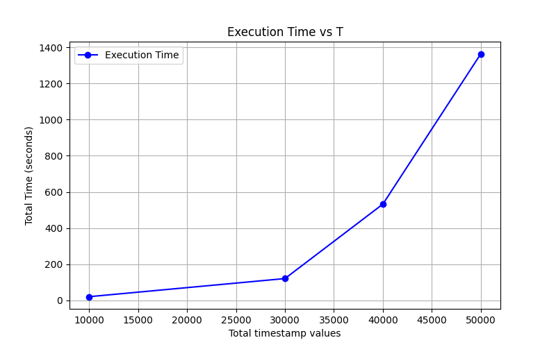
We evaluate the performance of our Integer Linear Programming (ILP) formulation on synthetically generated temporal networks. We used a Gurobi solver in its current configuration, the model scales effectively to instances comprising up to temporal edges, with total runtime remaining under minutes. The formulation demonstrates optimal performance in scenarios characterized by a relatively small number of activity intervals per vertex. For our standard benchmarking experiments, we fixed the number of activity intervals at and used an overlap coefficient of . Additionally, to assess the scalability of the approach under alternative structural conditions, we conducted a separate test with a reduced value and a larger graph containing more vertices and edges. Empirically, we observed that lower overlap coefficients lead to faster computational times; nonetheless, we maintained a minimum overlap of in most experiments to better reflect real-world temporal dynamics. Across all tested configurations, the ILP formulation consistently achieved high solution accuracy, with both precision and recall exceeding , indicating the correctness and robustness of the approach.
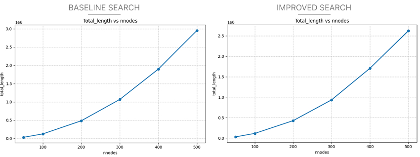
In the following, we compare the results of the k-Baseline and k-Inner heuristics of [14] with their improved versions using the heuristic algorithm. We will do a separate analysis for each of the considered algorithms. Starting with k-Baseline, we observe that, precision-wise the results are similar. This apparent discrepancy occurs because both sets of intervals are being compared against the ground-truth results, which remain considerably smaller in magnitude. The standard comparison metrics do not fully capture the practical significance of our improvements because both the initial approach and our method necessarily produce solutions that deviate substantially from the optimal (given the NP-hard nature of the problem and its known approximation hardness of any factor). Nevertheless, when examining the total interval length across all vertex variations, we observe a clear and consistent improvement. This improvement stems directly from our algorithm (as detailed in Section 5), which calculates the loss of every interval for each vertex and, for vertices containing intervals with zero loss, recalculates the activity timestamps and optimally reorders them using dynamic programming.
Comparative analysis of our approach against the baseline reveals consistent improvements in precision and recall metrics, which are represented by an average improvement that exceeds and peak differentials of more than in maximum values. We use Figure 4 for reference. Other relevant average comparisons are for recall, which stays the same for the Baseline and the Heuristic Improvement algorithm at . More significantly, our method demonstrates substantial optimization of the total interval length, reducing it from to , which constitutes a reduction of . This considerable decrease in total length, coupled with the consistent precision improvements, underscores the robustness and practicality of our algorithmic refinements.
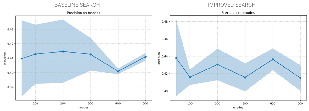
In the experimental phase aimed at enhancing the k-Inner algorithm, we adopted a slightly modified approach. Specifically, we conducted a dry run for all vertices with a loss value of zero, retaining the newly generated activity intervals only if they resulted in a lower total cost compared to the baseline established by the original k-Inner algorithm. This conservative strategy was employed as a safeguard, given that the original heuristic already achieves a high precision of approximately . In earlier iterations, we observed instances where modifying certain vertices adversely affected the interval structure, leading to significant reductions in overall precision. Despite these challenges, our modified heuristic yields slight but consistent improvements. However, given the already high baseline precision, these gains typically fall within a margin of approximately . To ensure robustness in evaluation, we extended the number of iterations and increased the total number of vertices analyzed. As shown in Figure 6, our approach surpasses the precision threshold for a limited number of vertices, after which the performance aligns closely with that of the original k-Inner algorithm. This convergence is expected, as the algorithm already performs near-optimally, leaving few opportunities for zero-loss interval modifications. Consequently, the impact on the total interval length remains minimal.

6 Conclusion and Future Works
We have considered -MinTimelineCover, a problem defined for complex data summarization. We have presented an ILP formulation for moderate size instances and we have designed an efficient heuristic based on local search. We have presented an experimental evaluation on synthetic data sets for both methods. Future works include an experimental evaluation on real-word datasets and an investigation of the performance of variants of our heuristics that extend the local search approach, for example when more than one vertex containing an interval of loss equal to is considered in this step.
References
- [1] Argyrios Deligkas, Michelle Döring, Eduard Eiben, Tiger-Lily Goldsmith, and George Skretas. Being an influencer is hard: The complexity of influence maximization in temporal graphs with a fixed source. Inf. Comput., 299:105171, 2024. doi:10.1016/J.IC.2024.105171.
- [2] Riccardo Dondi. Untangling temporal graphs of bounded degree. Theor. Comput. Sci., 969:114040, 2023. doi:10.1016/J.TCS.2023.114040.
- [3] Riccardo Dondi and Manuel Lafond. An FPT algorithm for temporal graph untangling. In Neeldhara Misra and Magnus Wahlström, editors, 18th International Symposium on Parameterized and Exact Computation, IPEC 2023, September 6-8, 2023, Amsterdam, The Netherlands, volume 285 of LIPIcs, pages 12:1–12:16. Schloss Dagstuhl – Leibniz-Zentrum für Informatik, 2023. doi:10.4230/LIPIcs.IPEC.2023.12.
- [4] Riccardo Dondi and Alexandru Popa. Timeline cover in temporal graphs: Exact and approximation algorithms. In Sun-Yuan Hsieh, Ling-Ju Hung, and Chia-Wei Lee, editors, Combinatorial Algorithms - 34th International Workshop, IWOCA 2023, Tainan, Taiwan, June 7-10, 2023, Proceedings, volume 13889 of Lecture Notes in Computer Science, pages 173–184. Springer, 2023. doi:10.1007/978-3-031-34347-6_15.
- [5] Riccardo Dondi and Alexandru Popa. Exact and approximation algorithms for covering timeline in temporal graphs. Annals of Operations Research, April 2024. doi:10.1007/s10479-024-05993-8.
- [6] Vincent Froese, Pascal Kunz, and Philipp Zschoche. Disentangling the computational complexity of network untangling. CoRR, abs/2204.02668, 2022. doi:10.48550/arXiv.2204.02668.
- [7] Petter Holme and Jari Saramäki. Temporal networks. CoRR, abs/1108.1780, 2011. arXiv:1108.1780.
- [8] Mohammad Mehdi Hosseinzadeh, Mario Cannataro, Pietro Hiram Guzzi, and Riccardo Dondi. Temporal networks in biology and medicine: a survey on models, algorithms, and tools. Netw. Model. Anal. Health Informatics Bioinform., 12(1):10, 2023. doi:10.1007/S13721-022-00406-X.
- [9] David Kempe, Jon M. Kleinberg, and Amit Kumar. Connectivity and inference problems for temporal networks. J. Comput. Syst. Sci., 64(4):820–842, 2002. doi:10.1006/JCSS.2002.1829.
- [10] Giorgio Lazzarinetti, Riccardo Dondi, Sara Manzoni, and Italo Zoppis. DLMinTC+: A deep learning based algorithm for minimum timeline cover on temporal graphs. Algorithms, 18(2):113, 2025.
- [11] Giorgio Lazzarinetti, Sara Manzoni, Italo Zoppis, and Riccardo Dondi. FastMinTC+: A fast and effective heuristic for minimum timeline cover on temporal networks. In Pietro Sala, Michael Sioutis, and Fusheng Wang, editors, 31st International Symposium on Temporal Representation and Reasoning, TIME 2024, October 28-30, 2024, Montpellier, France, volume 318 of LIPIcs, pages 20:1–20:18. Schloss Dagstuhl – Leibniz-Zentrum für Informatik, 2024. doi:10.4230/LIPIcs.TIME.2024.20.
- [12] Yike Liu, Tara Safavi, Abhilash Dighe, and Danai Koutra. Graph summarization methods and applications: A survey. ACM Comput. Surv., 51(3):62:1–62:34, 2018. doi:10.1145/3186727.
- [13] Othon Michail. An introduction to temporal graphs: An algorithmic perspective. Internet Math., 12(4):239–280, 2016. doi:10.1080/15427951.2016.1177801.
- [14] Polina Rozenshtein, Francesco Bonchi, Aristides Gionis, Mauro Sozio, and Nikolaj Tatti. Finding events in temporal networks: segmentation meets densest subgraph discovery. Knowl. Inf. Syst., 62(4):1611–1639, 2020. doi:10.1007/S10115-019-01403-9.
- [15] Polina Rozenshtein, Nikolaj Tatti, and Aristides Gionis. The network-untangling problem: from interactions to activity timelines. Data Min. Knowl. Discov., 35(1):213–247, 2021. doi:10.1007/S10618-020-00717-5.
- [16] Neil Shah, Danai Koutra, Tianmin Zou, Brian Gallagher, and Christos Faloutsos. Timecrunch: Interpretable dynamic graph summarization. In Longbing Cao, Chengqi Zhang, Thorsten Joachims, Geoffrey I. Webb, Dragos D. Margineantu, and Graham Williams, editors, Proceedings of the 21th ACM SIGKDD International Conference on Knowledge Discovery and Data Mining, Sydney, NSW, Australia, August 10-13, 2015, pages 1055–1064. ACM, 2015. doi:10.1145/2783258.2783321.
- [17] John Tang, Mirco Musolesi, Cecilia Mascolo, and Vito Latora. Temporal distance metrics for social network analysis. In Proceedings of the 2nd ACM workshop on Online social networks, pages 31–36, 2009.