Asynchronous Latency and Fast Atomic Snapshot

Bezerra, João Paulo; Freitas, Luciano; Kuznetsov, Petr; Rambaud, Matthieu

doi:10.4230/LIPIcs.DISC.2025.15

Asynchronous Latency and Fast Atomic Snapshot

João Paulo Bezerra

LTCI, Télécom Paris, Institut Polytechnique de Paris, France Luciano Freitas

Nomadic Labs, Paris, France Petr Kuznetsov

LTCI, Télécom Paris, Institut Polytechnique de Paris, France Matthieu Rambaud LTCI, Télécom Paris, Institut Polytechnique de Paris, France

Abstract

This paper introduces a novel, fast atomic-snapshot protocol for asynchronous message-passing systems. In the process of defining what “fast” means exactly, we spot a few interesting issues that arise when conventional time metrics are applied to long-lived asynchronous algorithms. We reveal some gaps in latency claims made in earlier work on snapshot algorithms, which hamper their comparative time-complexity analysis. We then come up with a new unifying time-complexity metric that captures the latency of an operation in an asynchronous, long-lived implementation. This allows us to formally grasp latency improvements of our atomic-snapshot algorithm with respect to the state-of-the-art protocols: optimal latency in fault-free runs without contention, short constant latency in fault-free runs with contention, the worst-case latency proportional to the number of active concurrent failures, and constant amortized latency.

Keywords and phrases:

Asynchronous systems, time complexity, atomic snapshot, crash faults

Funding:

João Paulo Bezerra: Mazars, TrustShare Innovation Chair.

Petr Kuznetsov: CHIST-ERA-22-SPiDDS-05 (REDONDA project) and Agence Nationale de la Recherche (ANR-23-CHR4-0009).

Copyright and License:

2012 ACM Subject Classification:

Theory of computation

\rightarrow

Distributed algorithms

Editor:

Dariusz R. Kowalski

Series and Publisher:

Leibniz International Proceedings in Informatics, Schloss Dagstuhl – Leibniz-Zentrum für Informatik

1 Introduction

The distributed snapshot abstraction [14, 26] allows us to determine a consistent view of the global system state. Originally proposed in the asynchronous fault-free message-passing context, it was later cast to shared-memory models [3] as a vector of shared variables, exporting an update operation that writes to one of them and a snapshot operation that returns the current vector state. Atomic snapshot can be implemented from conventional read-write registers in a wait-free manner, i.e., tolerating unpredictable delays or failures of any number of processes. By applying the reduction from shared memory to message-passing [6], one can get an asynchronous distributed atomic-snapshot implementation that tolerates up to a minority of faulty processes. The atomic-snapshot object (ASO) is, in a strong sense, equivalent to lattice agreement (LA) [8, 17]¹¹1Lattice agreement can be seen as a weak version of consensus, where decided values form totally ordered joins of proposed values in a join semi-lattice.: one can implement the other with no time overhead. A long line of results improve time and space complexities of ASO and LA algorithms in shared-memory [5, 4, 7] and message-passing [17, 21, 19, 16, 18] models.

In this paper, we focus on the latency of operations in message-passing ASO implementations. We propose an LA (and, thus, ASO) algorithm that is faster than (or matches) state-of-the-art solutions in all execution scenarios: with or without failures and with or without contention. The comparative analysis of our algorithm with respect to the existing work appeared to be challenging: as we show, earlier work considered diverging metrics and execution scenarios, and sometimes used over-simplified reasoning. We observed that conventional metrics [13, 6, 2] are not always suitable for long-lived asynchronous algorithms. Besides, prior latency analyses of ASO and LA algorithms [17, 21, 19, 16, 18] used different ways to measure time, which complicated the comparison. We therefore propose a unifying time-complexity analysis of prior asynchronous ASO and LA algorithms with respect to a new metric, which we take as a contribution on its own.

Table 1: Comparative time complexity of atomic-snapshot algorithms in asynchronous message-passing models. The table shows results for Single-Writer Multi-Reader (SWMR) implementations.

Fault-free

w/o contention

Fault-free

w/ contention

Worst-case

Amortized

constant

Faleiro et al. [17]

2

16

O(k)

yes

Imbs et al. [21]

2

O(n)

O(n)

no

Garg et al. [18]

\geq 6

\geq 8

O(k)

yes

Garg et al. [18] + Zheng et al. [27]

O(\log n)

O(\log n)

O(\log n)

no

Delporte et al. [16]

2

O(n)

O(n)

no

This paper

2

8

O(k)

yes

Lamport [25] proposed to measure time in asynchronous systems as the length of the longest chain of causally related messages, the metric used to to determine the best-case latency of consensus [25] and Crusader Agreement [1]. However, as we show in this paper, the metric may produce counter-intuitive results for protocols involving all-to-all communication. For instance, in the failure-free case, $n$ -process reliable broadcast [12] exhibits a causal chain of $n$ hops, even though, intuitively one expects it to terminate in one.

Building upon the classical approach by Canetti and Rabin [13], Abraham et al. [2] recently proposed an elegant metric to grasp the good-case latency of broadcast protocols. We observe, however, that the metric does not really apply to executions of long-lived abstractions, which may contain holes – periods of inactivity when no protocol messages are in transit. Moreover, we get diverging results when applying [2] and [13] to operation latency, i.e., the time between invocation and response events of a given operation.

We therefore extend the round-based approach to long-lived abstractions (such as ASO and LA) and establish a framework to measure the time between arbitrary events, subsequently showing that the results align with those from earlier classical metrics [6, 13].

To summarize, our main contribution is a novel LA (and, thus, ASO) protocol that is generally faster than prior solutions, i.e., it exhibits shorter latency of its operations in various scenarios. In our complexity analysis, we compared our protocol to the original long-lived LA algorithm by Faleiro et al. [17]²²2We consider the ASO protocol built atop the lattice agreement protocol proposed in [17]., the first direct message-passing ASO implementation by Delporte et al. [16], the ASO algorithm based on the set-constraint broadcast by Imbs et al. [21], and the ASO algorithms by Garg et al. based on generic construction of ASO from one-shot LA with constant latency in fault-free runs [18] or $\log{n}$ worst-case latency by Zheng et al. [27] (where $n$ is the number of processes).

As shown in Table 1, in a fault-free run, the latency of an operation of our protocol is the optimal two rounds if there is no contention and eight rounds in the presence of contention (four rounds if we ignore the “buffering” period when a value is submitted but not yet proposed), regardless of the number of contending operations. Moreover, the worst-case latency of our algorithm is proportional to the number of active failures $k$ , i.e., the number of faulty processes whose messages are received within the operation’s interval, therefore the amortized latency (averaged over a large number of operations in a long-lived execution) converges to the fault-free constant.

Our protocol can be seen as a novel combination of techniques employed separately in prior work. These include the use of generalized (long-lived) lattice agreement as a basis for ASO [23], the helping mechanism where all the learned lattice values are shared [23], relaying of messages to all replicas instead of quorum-based rounds [21, 18, 22, 15], and buffering proposed values until previous proposals get committed [17]. Similar to earlier proposals [17], our algorithm involves $O(n^{2})$ (all-to-all) communication, which is compensated by its constant (amortized) latency. An interesting open question is whether one can reduce the communication cost in good runs, while maintaining constant amortized latency.

The paper is organized as follows. In Section 2, we present our model assumptions, and in Section 3, we state the problem of atomic snapshot and relate it to generalized lattice agreement. In Section 4, we present our protocol and analyze its correctness. In Section 5, we discuss several gaps in the complexity analyses of earlier work. In Section 6, we present a comparative analysis of time metrics. Certain proofs and a detailed discussion of time complexity of earlier protocols are delegated to the appendix.

2 System Model

Processes and Channels.

We consider a system of $n$ processes (or nodes). Processes communicate by exchanging messages $m=(s,r,\textit{data})$ with a sender $s$ , a receiver $r$ , and a message content data.

A process is an automaton modeled as a tuple $(\mathcal{I},\mathcal{O},\mathcal{Q},q_{0},\pi)$ , where $\mathcal{I}$ is a set of inputs (messages and application calls) it can receive, $\mathcal{O}$ is a set of outputs (messages and application responses), $\mathcal{Q}$ is a (potentially infinite) set of possible internal states, $q_{0}\in\mathcal{Q}$ is an initial state and $\pi:2^{\mathcal{I}}\times\mathcal{Q}\rightarrow 2^{\mathcal{O}}\times\mathcal{Q}$ is a transition function mapping a set of inputs and a state to a set of outputs and a new state. Each process $i$ is assigned an algorithm $A_{i}$ which defines $(\mathcal{I},\mathcal{O},\mathcal{Q},q_{0},\pi)$ , a distributed algorithm is an array $[A_{1},...,A_{n}]$ .

Events and Configurations.

Application calls and responses are tuples $(i,\textit{aReq})$ and $(i,\textit{aRep})$ with a process identifier, a request, and a reply respectively.

An event $e$ is a tuple $(R,P,S)$ where $R$ is a set of received messages and/or application calls, $P$ is the set of nodes producing the event and $S$ is a set of messages sent and/or application responses. We denote $\textsf{receive}(e)$ as the set of messages received in the event, conversely, $\textsf{send}(e)$ is the set of messages sent. A message hop is a pair $(e,e^{\prime})$ in which $e^{\prime}$ receives at least one message that was sent in $e$ .

Messages in transit are stored in the message buffer.³³3We assume that every message in the message buffer is unique. A configuration $C$ is an $(n+1)$ -array $[M,s_{1},...,s_{n}]$ with the buffer’s state $M=C[0]$ and the local state $s_{i}=C[i]$ of each node $i$ ( $i=1,\ldots,n$ ). Let $C_{0}$ denote the initial configuration in which every $s_{i}$ is an initial state and the buffer $M$ is empty.

Executions.

An execution (or run) is an alternating sequence $C_{0}e_{1}C_{1}e_{2}...$ of configurations and events, where for each $j>0$ and $i=1,\ldots,n$ :

1.

$\textsf{receive}(e_{j})\subseteq C_{j-1}[0]$ ;
2.

$e_{j}.S$ consists of messages and application outputs that the nodes in $e_{j}.P$ produce, given their algorithms, their states in $C_{j-1}$ and their inputs in $e_{j}.R$ ; the nodes in $e_{j}.P$ carry their states from $C_{j-1}$ to $C_{j}$ , accordingly;
3.

for the nodes $i\notin e_{j}.P$ , $C_{j-1}[i]=C_{j}[i]$ .

Each triple $C_{j-1}e_{j}C_{j}$ is called a step. In this paper, we consider algorithms defined by deterministic automata, and we assume a default initial state. Thus, we sometimes skip configurations and simply write $e_{1}e_{2}\ldots$ .

In an infinite execution, a process is correct if it takes part in infinitely many steps, and faulty otherwise. We only consider infinite executions in which $f<n/2$ , where $f$ is the number of faulty processes and $n$ is the total number of processes. Moreover, in an infinite execution, messages exchanged among correct processes are eventually received, i.e., if there is an event $e$ from a correct process sending a message $m$ to another correct process, then there is $e^{\prime}$ succeeding $e$ such that $m\in\textsf{receive}(e^{\prime})$ .

We also assume that the communication channels neither alter nor create messages. Finally, we assume that the channels are FIFO: messages from a given source to a given destination arrive in the order they were sent. A FIFO channel can be implemented by attaching sequence numbers to messages, without extra communication or time overhead.

3 Lattice Agreement and Atomic Snapshot

3.1 Lattice Agreement

A join semi-lattice is defined as a tuple $(\mathcal{L},\sqsubseteq)$ , where $\sqsubseteq$ is a partial order on a set $\mathcal{L}$ , such that for any pair of values $u$ and $v$ in $\mathcal{L}$ , there exists a unique least upper bound $u\sqcup v\in\mathcal{L}$ ( $\sqcup$ is called the join operator). Also, $u$ and $v$ in $\mathcal{L}$ are said to be comparable if $u\sqsubseteq v\vee v\sqsubseteq u$ .

The (generalized) Lattice Agreement abstraction LA [17] defined over $(\mathcal{L},\sqsubseteq)$ can be accessed by every node with operation $\textsf{Propose}(v)$ , $v\in\mathcal{L}$ (we say that the node proposes $v$ ) which triggers the reply event $\textsf{Learn}(w)$ (we say that the node learns $w$ ). Each node may invoke Propose any number of times but does so sequentially, that is, it initiates a new operation only after the previous one has returned.⁴⁴4Following [23], without loss of generality, we slightly modified the conventional LA interface [8, 17] by introducing the explicit Propose operation that combine proposing and learning the values, the properties of the abstraction are adjusted accordingly. The abstraction must satisfy:

Definition 1 (Lattice Agreement (LA)).

$\blacksquare$

Validity. Any value learned by a node is the join of some set of proposed values that includes its last proposal.
$\blacksquare$

Stability. The values learned by any node increase monotonically, with respect to $\sqsubseteq$ .
$\blacksquare$

Consistency. All values learned are comparable, with respect to $\sqsubseteq$ .
$\blacksquare$

Liveness. If a correct node proposes $v$ , it eventually learns a value $w$ .

3.2 Atomic Snapshot Object (ASO)

An atomic snapshot object (ASO) stores a vector of values $R=[r_{1},...,r_{m}]$ and exports two operations: $\textsf{update}(i,v)$ and $\textsf{snapshot}()$ . The $\textsf{update}(i,v)$ operation writes the value $v$ in $R[i]$ and returns OK, and $\textsf{snapshot}()$ returns the entire vector $R$ . An ASO implementation guarantees that every operation invoked by a correct process eventually completes. It also ensures that each of its operations appears to take effect in a single instance of time within its interval, i.e., it is linearizable [20].

We say that an ASO is single writer SW (resp. multi writer MW) if for each of its registers $R[i]$ , only a single process can call $\textsf{update}(i,v)$ (resp. every process can call $\textsf{update}(i,v)$ ). In this paper, we focus mostly on SWMR atomic snapshot objects. In Table 1 we give results only for SWMR. A MWMR ASO can be devised from SWMR by adding an additional “read” phase when updating values (see Section 3.3 for more details).

Next, we show that ASO can be implemented on top of LA with no additional overhead.

3.3 From LA to ASO

To implement a SWMR ASO on top of LA, we build upon the transformation algorithm introduced in [23]. We consider a partially ordered set $\mathcal{L}^{*}$ of $(m+n)$ -vectors (recall that $m$ is the size of the ASO vector and $n$ is the number of nodes), defined as follows.

A vector position $\ell\in 1,\ldots,m$ is defined as a tuple $(w,v)\in R_{\ell}$ , where $v$ is an element of a value set $V$ equipped with a total order $\leq^{V}$ , and $w\in\mathbb{N}$ is the number of write operations on position $\ell$ . A total order on $R_{\ell}$ is defined in the natural way: for any two tuples $(w_{1},v_{1})\leq^{R_{\ell}}(w_{2},v_{2})\equiv(w_{1}<w_{2})\vee(w_{1}=w_{2}% \wedge v_{1}\leq^{V}v_{2})$ . For each process $i=1,\ldots,n$ , the vector position $m+i$ stores the number of snapshot operations executed by $i$ .

The lattice $\mathcal{L}^{*}$ of $(m+n)$ -position vectors is then the composition $R_{1}\times\ldots\times R_{m}\times\mathbb{N}^{n}$ . The partial order $\sqsubseteq^{*}$ on $\mathcal{L}^{*}$ is then naturally defined as the compositions of $<^{R_{1}}\times\ldots\times<^{R_{m}}\times\leq^{n}$ . The composed join operator $\sqcup^{*}$ is the composition of $\max$ operators, one for each position in the $(m+n)$ -position vectors. The construction implies a join semi-lattice [23].

In Algorithm 1, we show how to implement an SWMR atomic snapshot on top of LA defined over the semi-lattice $(\mathcal{L}^{*},\sqsubseteq^{*},\sqcup^{*})$ . For simplicity, we assume that $m=n$ , i.e., the size of the array is the total number of nodes, and that each node $i$ has a dedicated register $i$ where it can write. Elements of $\mathcal{L}^{*}$ are then $2n$ -vectors.

When a node $i$ calls $\textsf{update}($ i,v $)$ , it increments its local writing sequence number $w$ and proposes a $2n$ -vector with $(w,v)$ in position $i$ and initial values in all other positions to the LA object. The vector learned from this proposal is ignored. When the node $i$ calls $\textsf{snapshot}()$ , it increments its local reading sequence number $r$ proposes a $2n$ -vector with $r$ in position $n+i$ and initial values in all other positions to the LA object. The values in the first $n$ positions of the returned vector is then returned as the snapshot outcome.

Algorithm 1

\textsc{LA}\to\textbf{SW}\textbf{MR}

ASO conversion.

1:Distributed objects:

2: LA instance on

(\mathcal{L}^{*},\sqsubseteq^{*},\sqcup^{*})

3:upon startup

4:

w\leftarrow 0

5:

r\leftarrow 0

6:operation update(

i, v

)

7:

w\leftarrow w+1

8:

V\leftarrow

2n

-vector with

(w,v)

in position

i

and initial values in all other positions

9: LA.Propose

(V)

10:operation snapshot()

11:

r\leftarrow r+1

12:

V\leftarrow

2n

-vector with

r

in position

n+i

and initial values in all other positions

13: return

(\textsc{LA}.\textsf{Propose}(V))[1..n]

Algorithm 1 can be extended to implement a MWMR ASO: to update a position $j$ in the array, a node first takes a snapshot to get the current state, gets up-to-date sequence number in position $j$ and proposes its value with a higher sequence number. With this modification, the update operation takes two LA operations instead of one. We refer the reader to [23] for further details.

Theorem 2.

Algorithm 1 implements ASO.

Proof.

See Appendix A. $\hfill\blacktriangleleft$

4 LA Protocol

In Algorithm 2, we describe our protocol for solving LA. To guarantee amortized constant complexity, the protocol relies on two basic mechanisms, employed separately in earlier work [17, 23]. First, when a node receives a request (e.g., a value from the application), it first adds the request to a buffer ( $\mathit{MPool}$ ) and then relays it before starting a proposal. This ensures that “idle” nodes also help in committing the request. Second, the node relays every learned value so that nodes that are “stuck” can adopt values from other nodes.

4.1 Overview

The protocol is based on helping: every node tries to commit every proposed value it is aware of. As long as the node has active proposals that are not yet committed, it buffers newly arriving proposals in the local variable $\mathit{MPool}$ . Intuitively, in the worst case, an $\textsc{LA}.\textsf{Propose}$ operation has to wait until one of the concurrently invoked $\textsc{LA}.\textsf{Propose}$ operations complete. Once this happens, the currently buffered value is put in the local dictionary $\mathit{Pending}$ and shared with the other nodes (lines 31 and 32) via a PROPOSE message. In turn, the other nodes relay the message to each other (line 38). The dictionary maps a value to the number of times it is “supported” by the nodes (using PROPOSE messages). Once a value $v$ in the dictionary assembles a quorum of $n-f$ of $\langle\textbf{PROPOSE},v\rangle$ messages, i.e., $\mathit{Pending}[v]\geq n-f$ (line 39), the value is added to the $\mathit{Validated}$ variable. Once every value currently stored in $\mathit{Pending}$ is in $\mathit{Validated}$ (line 41), the operation completes with $\mathit{Validated}$ as the learned value. As the final element of the helping mechanism, each process broadcasts every value it learns (lines 45 and 51), ensuring that processes that might otherwise remain “stuck” can complete their current proposal.

In summary, the algorithm relies on four main ideas: 1) buffering incoming requests when already proposing, 2) sharing every received proposal so all processes are quickly aware of active ones, 3) initiating a new proposal only after all currently seen proposals have been validated, and 4) broadcasting learned values to help other processes make progress.

Message Complexity.

The protocol is comprised of three all-to-all communication phases: processes send and relay requests at lines 23 and 27, proposals at lines 32 and 38, and accepted values at lines 45 and 51. The total number of messages is therefore $O(n^{2})$ . However, a value in a PROPOSE message can include up to $n$ distinct requests, and a value in a ACCEPT message may have arbitrary size. Therefore, in the extended version [11], we present a refined protocol description in which processes exchange $O(n^{2})$ messages per individual request. This efficiency is achieved by relaying only the differences between current and previously received proposals and the learned values in phases $2$ and $3$ , thus eliminating redundant messages with the same requests.

Algorithm 2 Long-Lived LA: code for node

x

.

14:upon Startup

15:

\mathit{MPool},\mathit{Proposing},\mathit{Validated},\mathit{Learned}\leftarrow\perp

16:

\mathit{Pending}\leftarrow\emptyset

17:operation Propose(

v

)

18: SendRequest(

v

)

19: wait until

v\sqsubseteq\mathit{Learned}

20: return

\mathit{Learned}

21:operation SendRequest(

v

)

22:

\mathit{MPool}\leftarrow\mathit{MPool}\sqcup v

23: send

\langle

\textbf{REQUEST},v

\rangle

to every other node

24:upon Receive

\langle

\textbf{REQUEST},v

\rangle

from a node

25: if

v\not\sqsubseteq\mathit{MPool}\sqcup\mathit{Proposing}\sqcup\mathit{Learned}

then

26:

\mathit{MPool}\leftarrow\mathit{MPool}\sqcup v

27: send

\langle

\textbf{REQUEST},v

\rangle

to every other node

28:upon event

(\mathit{MPool}\neq\perp)\wedge(\mathit{Proposing}=\perp)

29:

\mathit{Proposing}\leftarrow\mathit{MPool}

30:

\mathit{MPool}\leftarrow\perp

31:

\mathit{Pending}[\mathit{Proposing}]\leftarrow 1

32: send

\langle

\textbf{PROPOSE},\mathit{Proposing}

\rangle

to every other node

33:upon Receive

\langle

\textbf{PROPOSE},v

\rangle

from a node

34: if

v\in\mathit{Pending}.\textsf{keys}()

then

35:

\mathit{Pending}[v]++

36: else

37:

\mathit{Pending}[v]\leftarrow 1

38: send

\langle

\textbf{PROPOSE},v

\rangle

to every node

39:upon exists

v

s.t.

\mathit{Pending}[v]=n-f

40:

\mathit{Validated}\leftarrow\mathit{Validated}\sqcup v

41:upon event

\bigsqcup\mathit{Pending}.\textsf{keys}()\sqsubseteq\mathit{Validated}

42: if

\mathit{Learned}\sqsubset\mathit{Validated}

then

43:

\mathit{Learned}\leftarrow\mathit{Validated}

44:

\mathit{Proposing}\leftarrow\perp

45: send

\langle

\textbf{ACCEPT},\mathit{Learned}

\rangle

to every node

46:upon Receive

\langle

\textbf{ACCEPT},w

\rangle

from a node

47: if

(\mathit{Proposing}\sqcup\mathit{Learned}\sqsubseteq w)

then

48:

\mathit{Validated}\leftarrow\mathit{Validated}\sqcup w

49:

\mathit{Learned}\leftarrow w

50:

\mathit{Proposing}\leftarrow\perp

51: send

\langle

\textbf{ACCEPT},\mathit{Learned}

\rangle

to every node

4.2 Correctness

Validity and Stability are immediate. We now proceed with Consistency and Liveness.

Lemma 3.

If nodes $i$ and $j$ learn, resp., values $w_{i}$ and $w_{j}$ , then $w_{i}$ and $w_{j}$ are comparable.

Proof.

Suppose that $(w_{i}\not\sqsubseteq w_{j})\wedge(w_{j}\not\sqsubseteq w_{i})$ . Then there must exist $v_{i}\sqsubseteq w_{i}$ and $v_{j}\sqsubseteq w_{j}$ such that $v_{i}\not\sqsubseteq w_{j}$ and $v_{j}\not\sqsubseteq w_{i}$ .

Let $Q_{i}$ (resp. $Q_{j}$ ) be the quorum $i$ used to include $v_{i}$ $\mathit{Validated}$ at line 39. Since $Q_{i}\cap Q_{j}\neq\emptyset$ , there is a common node $x$ that sent $\langle\textbf{PROPOSE},v_{i}\rangle$ to $i$ and $\langle\textbf{PROPOSE},v_{j}\rangle$ to $j$ , but since channels are FIFO, either $i$ received $v_{j}$ or $j$ received $v_{i}$ from $x$ before learning a value, therefore adding the value to $\mathit{Pending}$ . Suppose it was $i$ that received $v_{j}$ before $v_{i}$ , from the condition of line 41, $i$ could not have learned $w_{i}$ if $v_{j}\not\sqsubseteq\mathit{Validated}$ . $\hfill\blacktriangleleft$

Lemma 4.

If a correct node $x$ sets $\mathit{Proposing}=v$ , $x$ eventually learns a value with $v$ .

Proof.

A node $x$ sends a PROPOSE message to every other node whenever it adds a new value to $\mathit{Pending}$ (line 38). If $x$ is correct, it will receive at least $n-f$ PROPOSE messages for every value in $\mathit{Pending}$ , adding the value to $\mathit{Validated}$ . Therefore, the condition in line 41 is never satisfied from some point on only if $x$ keeps adding a new value to $\mathit{Pending}$ before all the current ones are validated.

Since each node proposes only one value at a time (until it learns a value, lines 28, 44, 50), for $x$ to indefinitely add new values to $\mathit{Pending}$ , there must be at least one other node that keeps learning values and proposing new ones. Without loss of generality, let $y$ be one such node. Since faulty nodes eventually crash and stop taking steps, $y$ must be correct. Every time $y$ learns a new value $w$ it sends $\langle\textbf{ACCEPT},w\rangle$ to $x$ , and because channels are FIFO, $x$ receives the ACCEPT message before the new value proposed by $y$ . Eventually (because $x$ sent its proposal to $y$ ), one of the received values $w$ contains $x^{\prime}s$ $\mathit{Proposing}$ and the condition on line 46 is satisfied, $x$ then learns $w$ . $\hfill\blacktriangleleft$

Lemma 5.

If a correct node calls $\textsf{Propose}(v)$ , it eventually sets $\mathit{Proposing}=v^{\prime}$ , $v\sqsubseteq v^{\prime}$ .

Proof.

Let a correct node $x$ call $\textsf{Propose}(v)$ , $x$ then includes $v$ in $\mathit{MPool}$ (line 22). If $x$ is not currently proposing, that is, the current value of $\mathit{Proposing}$ is $\perp$ , then it meets the condition in line 28 and immediately sets $\mathit{Proposing}=\mathit{MPool}$ . Otherwise, by Lemma 4, it eventually learns a value and sets $\mathit{Proposing}=\perp$ in lines 44 and 50, thus meeting the condition in line 28 and setting $\mathit{Proposing}=\mathit{MPool}$ . $\hfill\blacktriangleleft$

Lemmas 3, 4 and 5 imply:

Theorem 6.

Algorithm 2 implements Generalized Lattice Agreement.

Corollary 7.

Algorithms 1 and 2 implement Atomic Snapshot.

4.3 Time Metric

We now define the latency metric we are going to use in evaluating time complexity. Our metric is inspired by the metric proposed by Abraham et al. [2] (which in turn rephrases the original metric by Canetti and Rabin [13]). The distinguishing feature of our approach is that it also applies to long-lived executions and executions with holes (illustrated in Figure 1).⁵⁵5In Section 6, we show that the three metrics are equivalent in “hole-free” executions.

Algorithm 3 describes the iterative method that assigns rounds to events in an execution. We give an informal description of the metric below.

Definition 8 (Iterative Round Assignment - Informal).

Algorithm 3 assigns round $0$ to the initial event, and defines the end of round $i$ as the last event that receives a message sent in round $i-1$ . In addition, if there are no more messages to be received (or in transit), the event inherits the round number of its immediate predecessor.

Algorithm 3 Iterative Round Assignment (IRA).

52:

e_{0}^{*}:=e_{0}

53:

e_{0}

is assigned round

0

54:

r:=0

55:for i=1… do

56: if

e_{i}

does not receive a message then

57:

e_{i}

is assigned round

r

58: else

59: Let

e_{j}

be the oldest event from which

e_{i}

receives a message

60: Let

r^{\prime}

be the round assigned to

e_{j}

(r^{\prime}\leq r)

61: Let

e^{\prime}

be the most recent event among

e_{r^{\prime}}^{*}

and

e_{j}

62: All events after

e^{\prime}

and up to

e_{i}

receive round

r^{\prime}+1

63:

e_{r^{\prime}+1}^{*}:=e_{i}

64:

r=r^{\prime}+1

Refer to caption — Figure 1: Example of round assignment using IRA. Arrows represent message transmissions and the number below an event corresponds to its round. A “hole” in communication appears betwen events $e_{3}$ and $e_{5}$ .

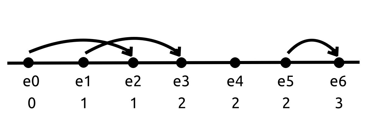
Definition 9 (IRA - Arbitrary Events).

To measure the latency between two events $e_{i}$ and $e_{j}$ , we assign rounds according to Algorithm 3, starting from $e_{i}$ , with all events up to and including $e_{i}$ receiving round $0$ . The latency between $e_{i}$ and $e_{j}$ is then given by the round assigned to $e_{j}$ .

We say that an application request (or simply request, when there is no ambiguity) completes once the receiving node learns a value which includes the request. For a specific node $i$ , we are interested in measuring the latency between the event $e_{C}$ in which $i$ receives a value $v$ from the application software, and an event $e_{R}$ , in which $i$ learns a value $w$ with $v$ .

4.4 Time Complexity of Algorithm 2

We define latency as the number of rounds spanning between the moment a correct process receives an application call and the moment it returns from the operation. In evaluating the latency of our protocol, we consider two types of executions: (1) the fault-free case, when all processes are correct, and (2) the worst-case, when only a majority of processes are correct.

A snapshot operation op precedes another operation $\textit{op}^{\prime}$ if the response event of op happens before the call event for $\textit{op}^{\prime}$ . Two operations are said to be concurrent if none precedes the other. For ASO protocols, we analyze latency in fault-free runs of an operation op in two distinct scenarios: (a) without contention, i.e., when no other operation overlaps in time with op, and (b) with contention, i.e., when there might be an arbitrary number of concurrent operations.

Garg et al. [19] use the notion of amortized time complexity, i.e., the average operation latency taken over a large number of operations in an execution. In some protocols, including ours, the latency of an operation is only affected by the number of faulty processes whose messages are received during the operation’s interval (we call these processes active-faulty). Intuitively, faulty processes take a finite amount of steps, so in these protocols a failure can only affect a finite number of operations. In this paper, we also distinguish ASO protocols with constant time complexity. In Appendix B, we establish the optimality of our protocol under no-contention and prove the following results:

Theorem 10.

An operation completes in at most $2$ rounds in fault-free runs w/o contention.

Consider an execution of our algorithm, and let $F$ ( $|F|\leq f$ ) be its set of faulty processes.

Theorem 11.

An operation op takes at most $8$ rounds to complete if, during its interval, no correct node receives a message from a faulty one.

We say that there are $k$ active faulty nodes during an operation op if, in between the call and return events for op, a message is received from a total of $k$ distinct faulty nodes.

Theorem 12.

An operation op takes $O(k)$ rounds to complete, where $k$ is the number of active faulty nodes during op.

Corollary 13.

Algorithms 1 and 2 together have an amortized time complexity of $8$ rounds.

5 Measuring Latency of ASO Protocols

We conclude the paper with an overview of time complexity of earlier LA and ASO protocols [17, 16, 21, 18, 19]. We highlight certain gaps in their latency analyses and discuss the ways to fix them. Formalities and proofs can be found in the full version [11].

The First Message-Passing LA Protocol.

Faleiro et al. [17] came up with the first LA implementation for asynchronous message-passing systems. They use the metric of [6] to measure latency and conclude that it takes $O(n)$ rounds to output from a lattice agreement operation in their protocol.

We show the somewhat surprising result that this protocol has constant latency of $16$ rounds in fault-free runs. The upper bound holds as long as no message from faulty processes is received during the interval of the operation, implying that their LA protocol has constant amortized time complexity. We conjecture that the protocol has $O(k)$ worst-case latency, where $k$ is the number of actual failures in the execution.

The First Direct ASO Implementation.

Delporte et al. [16] is the first paper to directly implement ASO in message passing systems, instead of using an atomic register implementation [6] and the shared-memory snapshot construction [3].

In fault-free runs without contention, the latency of their protocol is only $2$ rounds. In fault-free runs with contention, we support the claim of a bound of $O(n)$ rounds from [19].

ASO with SCD-Broadcast.

Imbs et al. [21] introduce the abstraction of Set Constrained Delivery Broadcast ( $\textsc{SCD}-\textsc{Broadcast}$ ), and show that it allows for implementing LA and ASO with no complexity overhead. In their complexity analysis, they assume bounded message delays and show that the latency of their ASO algorithm in faulty-free and contention-free runs is $2$ rounds. We show that an operation of their resulting ASO algorithm can take $\Omega(n)$ rounds in fault-free runs with contention. We conjecture that this bound is tight, and so the time complexity of their ASO protocol is $\Theta(n)$ .

A Generic ASO Algorithm.

Garg et al. [18, 19] give a generic construction for atomic snapshot which uses any one-shot LA protocol as a building block (with constant latency overhead). The protocol thus inherits the asymptotic complexity of the underlying LA algorithm. They also provide a protocol for one-shot LA with $2$ rounds latency in fault-free runs (using [13]’s metric). Their protocol requires 2 rounds of communication plus two lattice agreement invocations in the good case w/o contention and three lattice invocations with contention, making it at least 6 and 8 message delays, respectively.

For the worst-case latency analysis, they assume an additional requirement over communication channels: if a process executes $\textsf{send}(m)$ , sending $m$ to a correct process, then $m$ is eventually received (even if the sender is faulty). Using this assumption, they show a worst-case latency of $O(\sqrt{f})$ for their LA protocol.

In this paper, we assume a weaker channel that only guarantees delivery of messages among correct processes. We show that under this model, the LA protocol of [18] has an execution that takes $\Omega(f)$ rounds. We conjecture the upper bound of their protocol to be $O(f)$ , and also that when using the stronger assumption, both our (Section 4) and [21]’s protocol have $O(\sqrt{f})$ worst-case latency.

The generic ASO construction may also be combined with the one-shot LA protocol presented in [27], which has worst-case latency of $O(\log f)$ , providing an object whose update and snapshot operations take $O(\log f)$ in both fault-free fault-prone executions. For the sake of completeness, we also provide the time complexity analysis for the one-shot LA protocols from [17] and [21] in the full version [11].

6 Comparative Analysis of Time Measurement Metrics

In this section, we recall metrics used in the literature [6, 13, 2, 24] for measuring time in asynchronous systems. We exhibit executions where the metrics by Attiya et al. [6] and Canetti and Rabin [13] yield arbitrary results due to the presence of holes – “periods of silence” during which no messages are in transit – which are common in long-lived protocols. We show that in a subset of executions without holes, which we refer to as covered executions, these metrics align with the one proposed by Abraham et al. [2]. This is not surprising, as these metrics were designed for distributed tasks, which assume finite hole-free executions. We also recall Lamport’s longest causal chain metric [24] and show that it is not suitable for comparing the ASO protocols we consider here.

Next, we show that the metric from [2] diverges from [6] and [13] when naïvely applied to measure time between arbitrary events. We then show that, after employing our refined method from Section 4.3 (Definition 9), they match when measuring rounds between arbitrary events in covered executions. Finally, we show that both our metric and that of [2] yield equivalent results in cases where [2] is applicable.

Altogether, we establish that our metric generalizes [2] and aligns with classical metrics [6, 13] when applied to distributed tasks. A summary of the comparative analysis is presented in Table 2. Proofs are provided in the extended version [11].

Table 2: Comparison between asynchronous time metrics. Metrics that are timed make use of time assignments to determine the number of rounds between events. We compare each metric against CR, evaluating the number of rounds resulting from applying them over entire (covered) executions and between arbitrary events. Blue stands for “good” features and red – for “bad” ones. The equivalence of NTR to CR holds as long as one uses Definition 9.

Timed

Equivalent to CR

(Covered Executions)

Equivalent to CR

(Arbitrary Events)

Admits

Holes

CR [13]

Yes

-

No

Round [6, 9]

Yes

No

NTR [2]

No

Yes

No

LCC [25]

No

Yes

IRA

No

Yes

6.1 Definitions

Timed Executions.

We assume a global clock, not accessible to the nodes. A timed event $\overline{e}$ is a pair $(t,e)$ in which $t$ is a non-negative real number, we also say that $\overline{e}$ is a time assignment of $e$ . A timed execution is an alternating sequence $C_{0}\overline{e}_{1}C_{1}\dots$ where $\overline{e}_{1}=(t_{1},e_{1}),\overline{e}_{2}=(t_{2},e_{2}),\dots$ , where events $e_{1},e_{2},\ldots$ are equipped with monotonically increasing times $t_{1},t_{2},\ldots$ :

1.

$t_{m}>t_{l}$ whenever $m>l$ ;
2.

$t_{l}\rightarrow\infty$ as $l\rightarrow\infty$ .⁶⁶6We require this property to avoid the case where a never-terminating execution has a finite time duration.

A time assignment of $E$ is a timed execution $\overline{E}$ in which every event $e_{i}$ in $E$ is matched with a timed event $(t_{i},e_{i})$ in $\overline{E}$ and the sequences of configurations in $E$ and $\overline{E}$ are the same. Notice that an execution allows for infinitely many time assignments.

Let $m$ be a message sent in $\overline{e}_{l}$ and received in $\overline{e}_{m}$ , the delay of $m$ is then defined as $t_{m}-t_{l}$ . For a finite timed execution $\overline{E}=C_{0}\overline{e}_{1}...\overline{e}_{l}C_{l}$ , we define $t_{\textit{start}}(\overline{E})=t_{1}$ , $t_{\textit{end}}(\overline{E})=t_{l}$ (we use $t_{\textit{start}}$ and $t_{\textit{end}}$ when there is no ambiguity) and $\textit{duration}(\overline{E})=t_{\textit{end}}-t_{\textit{start}}$ .

In the subsequent discussion, given an execution $E$ , let $\mathcal{T}(E)$ denote the set of all timed executions $\overline{E}$ based on $E$ .

Time Metrics.

It is conventional to measure the execution time by the number of communication rounds, typically calculated using the “longest message delay.” These metrics can be applied to both executions and timed executions. The first metric we consider is defined in Definition 14 [6]. When applied to timed executions, this metric assumes a known upper bound on message delays, which can be normalized to one time unit without loss of generality. To apply this metric to an execution, we consider the maximum duration of all possible timed executions that adhere to the upper-bound communication constraint.

Definition 14 (Round metric).

Given a timed execution $\overline{E}$ , in which the maximum message delay is bounded by one unit of time, $\overline{E}$ takes $\textit{duration}(\overline{E})$ rounds.

By extension, an execution $E$ takes $\sup_{\overline{E}\in\mathcal{T}(E)}{\textit{duration}(\overline{E})}$ rounds.

In the metric proposed by Attiya and Welch [9, 10], the time assignments are scaled so that the maximum message delay is always $1$ , thus, the metric produces the same results for executions as Definition 14. A more general metric introduced by Canetti and Rabin [13] captures the time complexity of any finite execution. Let $\overline{E}$ be a timed execution, and let $\delta_{\overline{E}}$ be the maximum message delay in it. Then $\overline{E}$ takes $\textit{duration}(\overline{E})/\delta_{\overline{E}}$ CR rounds.

Definition 15 (CR metric).

A finite execution $E$ takes $\sup_{\overline{E}\in\mathcal{T}(E)}{\textit{duration}(\overline{E})/\delta_{% \overline{E}}}$ rounds, where $\delta_{\overline{E}}$ is the maximum message delay of each corresponding timed execution.

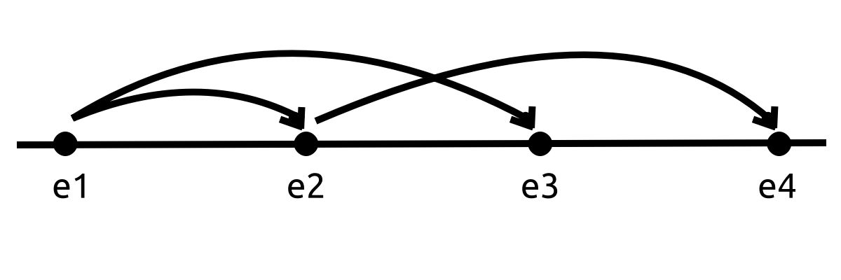
Example 16.

Figure 2 shows an execution with four events, where we assign a delay of $\delta$ to the message exchanges $(e_{1},e_{3})$ and $(e_{2},e_{4})$ , and a delay of $\delta-\epsilon$ ( $\epsilon>0$ ) to $(e_{1},e_{2})$ . By making $\epsilon$ arbitrarily small, the number of rounds in this execution converges to $2$ in the CR metric. The same result is obtained in the Round metric by setting $\delta=1$ .

Recently, Abraham et al. [2] proposed an approach that can be applied to executions without relying on time assignments. We call this metric non-timed rounds (NTR):

Definition 17 (NTR metric).

Given an execution $E$ , each event in $E$ is assigned a round number as follows:

$\blacksquare$

The first event $e_{0}$ is assigned round $0$ . We also write $e_{0}^{*}=e_{0}$ ;
$\blacksquare$

For any $r\geq 1$ , let $e_{r}^{*}$ be the last event where a message of round $r-1$ is delivered. All events after $e_{r-1}^{*}$ until (and including) event $e_{r}^{*}$ are in round $r$ .

The number of rounds in $E$ is the round assigned to its last event.

Example 18.

Coming back to Figure 2, if we assign a round to each event based on Definition 17 then $e_{1}$ gets round $0$ , $e_{2}$ and $e_{3}$ get round $1$ and $e_{4}$ is assigned round $2$ . The execution has therefore $2$ rounds according to NTR.

Lamport [25] proposed a metric for latency based on the causal chain of messages. The Longest Causal Chain (LCC) was used to show best-case latency of protocols such as consensus [25] and Crusader Agreement [1].

Definition 19 (Longest Causal Chain).

Let $e$ be an event in $E$ and $M$ the set of messages received by $e$ , then $e$ is assigned round $k+1$ , where $k$ is the maximum round of an event originating a message in $M$ . If $M=\emptyset$ , then $k=0$ . The number of rounds in an execution becomes the highest round assigned to one of its events.

This metric, however, diverges from CR and NTR.

Example 20 (Reliable Broadcast).

In the reliable broadcast primitive [12], a dedicated source broadcasts a message and, if the source is correct, then all correct nodes should deliver the message. Furthermore, if a correct process delivers a message, then every correct process eventually delivers it. The following protocol satisfies this property:

$\blacksquare$

When the source invokes broadcast( $m$ ), it delivers $m$ and sends it to everyone;
$\blacksquare$

When a process receives $m$ for the first time, it delivers $m$ and sends it to everyone.

In Figure 3, we depict an execution of this protocol with four processes: $p_{1}$ , $p_{2}$ , $p_{3}$ and $p_{4}$ . Here, $p_{1}$ is the source and broadcasts $m$ , the message is received by $p_{2}$ which then sends $m$ to everyone. Process $p_{3}$ receives $m$ from $p_{2}$ before receiving it from $p_{1}$ , and finally, $p_{4}$ receives $m$ from $p_{1}$ in the last event. This execution has $2$ LCC rounds, while having $1$ round according to CR and NTR.

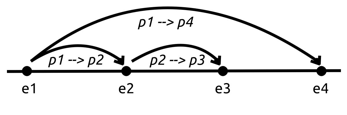
Example 20 shows that the LCC metric diverges from the others in cases where a fast exchange of messages happens in the interval of one slow message. This is the case for several ASO protocols in the literature (including ours) which heavily rely on relaying values to speed up the validation phase, making the metric unsuitable for our use case. On the other hand, CR and NTR provide equivalent results in covered executions, described next.⁷⁷7The Round and CR metrics also provide equivalent results in covered executions [11].

6.2 Covered Executions and Holes

Consider an execution $E=C_{0}e_{1}C_{1}...e_{l}C_{l}$ illustrated in Figure 4(a) where no process receives a message from another process, i.e., events may add messages to the buffer but no event removes a message from it. $\delta_{\overline{E}}$ is not defined in any time assignment $\overline{E}$ .

Now consider an execution $E^{\prime}=C_{0}e_{1}C_{1}...e_{l}C_{l}...e_{m}C_{m}$ in which:

$\blacksquare$

A message $m$ is sent in $e_{1}$ and received in $e_{l}$ ;
$\blacksquare$

A message $m^{\prime}$ is sent in $e_{l+1}$ and received in $e_{m}$ ;
$\blacksquare$

No message from $e_{1}...e_{l}$ is received in $e_{l+1}...e_{m}$ .

In this example, illustrated in Figure 4(b) with $5$ events, $\delta_{\overline{E^{\prime}}}$ exists for any time assignment of $E^{\prime}$ , but we can still assign an arbitrary time difference to $e_{l}$ and $e_{l+1}$ without affecting $\delta_{\overline{E^{\prime}}}$ , which results in the number of CR rounds to be unbounded.

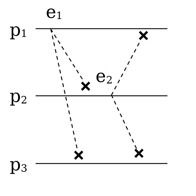
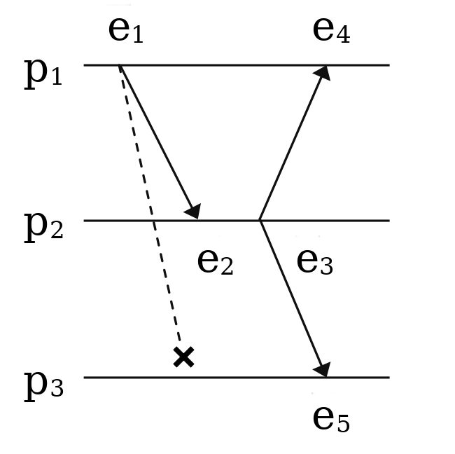
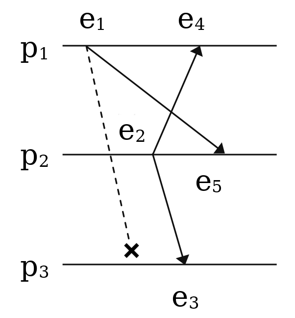
The two executions in the examples above have events whose time difference is unrelated to message delays. By consequence, the duration of these executions can grow irrespective of any bound imposed by message exchanges. Similarly, in Figure 4(b), since there is no message being received in $e_{3}e_{4}e_{5}$ from $e_{1}e_{2}$ , there is no round assignment defined when using NTR to $e_{3}$ , $e_{4}$ and $e_{4}$ .

We then restrict the analysis of these metrics to executions that are covered. Formally:

Definition 21 (Covered Execution).

A hole in an execution is a pair $(e_{l},e_{l+1})$ in which no event in $e_{l+1}...$ receives a message from $...e_{l}$ , in other words, there are no message hops among the two sequence of events. An execution is covered iff it has no holes.

Abraham et al. [2] introduce NTR as an equivalent to CR, however, no formal proof is provided. The next result corroborates this claim in covered executions. Later in Example 24, we show that using NTR naively to measure time between events may not match CR.

Theorem 22.

A finite covered execution $E$ has $k$ CR rounds iff it has $\lceil k\rceil$ NTR rounds.

6.3 Time Between Arbitrary Events

In long-lived executions (such as those of atomic snapshot algorithms) we are interested in measuring time between two events, for instance, between an application call and response. Definition 15 can easily be adapted to measure the number of rounds between two events as follows:

Definition 23 (Generalized CR metric).

Let $E$ be an execution, let $\mathcal{T}(E)$ denote the set of all timed executions $\overline{E}$ based on $E$ , and $\delta_{\overline{E}}$ - the maximum message delay in $\overline{E}$ . Let $e_{i}$ and $e_{j}$ ( $j>i$ ) be events in $E$ , and $t_{i}$ and $t_{j}$ time assignments in $\overline{E}$ for them respectively. Then we say that in between $e_{i}$ and $e_{j}$ there are: $\sup_{\overline{E}\in\mathcal{T}(E)}(t_{j}-t_{i})/\delta_{\overline{E}}$ CR rounds.

An appealing way of defining time between two events $e_{i}$ and $e_{j}$ using a non-timed metric is to assign rounds according to NTR, and then take the difference of rounds assigned to $e_{i}$ and $e_{j}$ . As illustrated in Example 24, this definition can diverge from generalized CR.

Example 24.

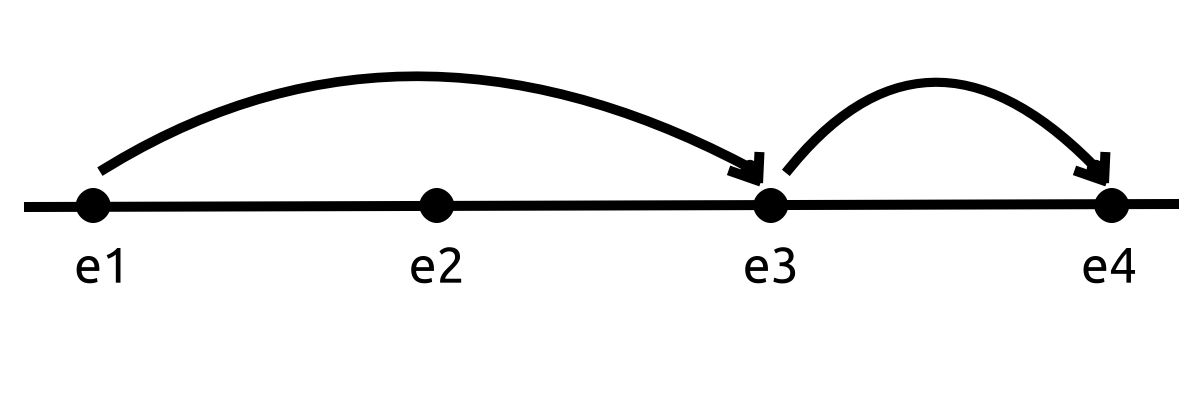
Consider the execution shown in Figure 5. We can assign times to $e_{1}$ , $e_{3}$ and $e_{4}$ such that the two message hops have delay of $\delta$ . Now consider the number of rounds between $e_{2}$ and $e_{4}$ , since we can assign a time for $e_{2}$ that is arbitrarily close to $e_{1}$ ’s assignment, there are $2$ CR rounds between $e_{2}$ and $e_{4}$ . However, the round assignments using NTR to $e_{2}$ and $e_{4}$ are $1$ and $2$ respectively, so simply taking the difference between them leads to a value that diverges from CR.

We then give the following definition, using the approach described in Section 4.3:

Definition 25 (Generalized NTR).

Given an execution $E$ , let $e_{i}$ and $e_{j}$ ( $j>i$ ) be events in $E$ . The number of rounds between $e_{i}$ and $e_{j}$ is given by the round assigned to $e_{j}$ according to the following:

$\blacksquare$

All events up to (and including) $e_{i}$ are assigned round $0$ . We also write $e_{0}^{*}=e_{i}$ ;
$\blacksquare$

For any $r\geq 1$ , let $e_{r}^{*}$ be the last event where a message of round $r-1$ is delivered. All events after $e_{r-1}^{*}$ until (and including) event $e_{r}^{*}$ are in round $r$ .

Theorem 26.

Let $E$ be a covered execution and $e_{i}$ and $e_{j}$ ( $j>i$ ) be events of $E$ . There are $k$ rounds in between $e_{i}$ and $e_{j}$ according to CR (Definition 23) iff there are $\lceil k\rceil$ rounds in between them according to NTR (Definition 25).

6.4 Relating IRA to NTR

Theorem 27.

Let $E$ be a finite covered execution and suppose that all events of $E$ are assigned rounds according to IRA after all iterations of the algorithm. It holds that:

1.

Round $0$ is composed only of $e_{0}$ (the initial event).
2.

The final event of round $i+1$ is the last event to receive a message from round $i$ .

Corollary 28.

IRA and NTR assign the same rounds to events in covered executions.

References

[1] Ittai Abraham, Naama Ben-David, Gilad Stern, and Sravya Yandamuri. On the round complexity of asynchronous crusader agreement. Cryptology ePrint Archive, 2023.
[2] Ittai Abraham, Kartik Nayak, Ling Ren, and Zhuolun Xiang. Good-case latency of byzantine broadcast: a complete categorization. CoRR, abs/2102.07240, 2021. arXiv:2102.07240.
[3] Yehuda Afek, Hagit Attiya, Danny Dolev, Eli Gafni, Michael Merritt, and Nir Shavit. Atomic snapshots of shared memory. J. ACM, 40(4):873–890, 1993. doi:10.1145/153724.153741.
[4] James Aspnes, Hagit Attiya, Keren Censor-Hillel, and Faith Ellen. Limited-use atomic snapshots with polylogarithmic step complexity. J. ACM, 62(1):3:1–3:22, 2015. doi:10.1145/2732263.
[5] James Aspnes and Keren Censor-Hillel. Atomic snapshots in o(log3 n) steps using randomized helping. In Yehuda Afek, editor, Distributed Computing - 27th International Symposium, DISC 2013, Jerusalem, Israel, October 14-18, 2013. Proceedings, volume 8205 of Lecture Notes in Computer Science, pages 254–268. Springer, 2013. doi:10.1007/978-3-642-41527-2_18.
[6] Hagit Attiya, Amotz Bar-Noy, and Danny Dolev. Sharing memory robustly in message-passing systems. J. ACM, 42(1):124–142, January 1995. doi:10.1145/200836.200869.
[7] Hagit Attiya, Faith Ellen, and Panagiota Fatourou. The complexity of updating snapshot objects. J. Parallel Distributed Comput., 71(12):1570–1577, 2011. doi:10.1016/J.JPDC.2011.08.002.
[8] Hagit Attiya, Maurice Herlihy, and Ophir Rachman. Atomic snapshots using lattice agreement. Distributed Comput., 8(3):121–132, 1995. doi:10.1007/BF02242714.
[9] Hagit Attiya and Jennifer Welch. Distributed computing: fundamentals, simulations, and advanced topics, volume 19. John Wiley & Sons, 2004.
[10] Hagit Attiya and Jennifer L Welch. Multi-valued connected consensus: A new perspective on crusader agreement and adopt-commit. In 27th International Conference on Principles of Distributed Systems, 2024.
[11] João Paulo Bezerra, Luciano Freitas, and Petr Kuznetsov. Asynchronous latency and fast atomic snapshot. arXiv preprint arXiv:2408.02562, 2024.
[12] Christian Cachin, Rachid Guerraoui, and Luís Rodrigues. Introduction to reliable and secure distributed programming. Springer Science & Business Media, 2011.
[13] Ran Canetti and Tal Rabin. Fast asynchronous byzantine agreement with optimal resilience. In Proceedings of the twenty-fifth annual ACM symposium on Theory of computing, pages 42–51, 1993. doi:10.1145/167088.167105.
[14] K. Mani Chandy and Leslie Lamport. Distributed snapshots: Determining global states of distributed systems. ACM Trans. Comput. Syst., 3(1):63–75, 1985. doi:10.1145/214451.214456.
[15] George Danezis, Lefteris Kokoris-Kogias, Alberto Sonnino, and Alexander Spiegelman. Narwhal and tusk: a dag-based mempool and efficient BFT consensus. In EuroSys, pages 34–50. ACM, 2022. doi:10.1145/3492321.3519594.
[16] Carole Delporte-Gallet, Hugues Fauconnier, Sergio Rajsbaum, and Michel Raynal. Implementing snapshot objects on top of crash-prone asynchronous message-passing systems. IEEE Transactions on Parallel and Distributed Systems, 29(9):2033–2045, 2018. doi:10.1109/TPDS.2018.2809551.
[17] Jose M. Faleiro, Sriram Rajamani, Kaushik Rajan, G. Ramalingam, and Kapil Vaswani. Generalized lattice agreement. In Proceedings of the 2012 ACM Symposium on Principles of Distributed Computing, PODC ’12, pages 125–134, New York, NY, USA, 2012. Association for Computing Machinery. doi:10.1145/2332432.2332458.
[18] Vijay Garg, Saptaparni Kumar, Lewis Tseng, and Xiong Zheng. Amortized constant round atomic snapshot in message-passing systems. arXiv preprint arXiv:2008.11837, 2020. arXiv:2008.11837.
[19] Vijay K. Garg, Saptaparni Kumar, Lewis Tseng, and Xiong Zheng. Fault-tolerant snapshot objects in message passing systems. In 2022 IEEE International Parallel and Distributed Processing Symposium (IPDPS), pages 1129–1139, 2022. doi:10.1109/IPDPS53621.2022.00113.
[20] Maurice Herlihy and Jeannette M. Wing. Linearizability: A correctness condition for concurrent objects. ACM Trans. Program. Lang. Syst., 12(3):463–492, 1990. doi:10.1145/78969.78972.
[21] Damien Imbs, Achour Mostéfaoui, Matthieu Perrin, and Michel Raynal. Set-constrained delivery broadcast: Definition, abstraction power, and computability limits. In Proceedings of the 19th International Conference on Distributed Computing and Networking, pages 1–10, 2018. doi:10.1145/3154273.3154296.
[22] Idit Keidar, Eleftherios Kokoris-Kogias, Oded Naor, and Alexander Spiegelman. All you need is DAG. In PODC, pages 165–175. ACM, 2021. doi:10.1145/3465084.3467905.
[23] Petr Kuznetsov, Thibault Rieutord, and Sara Tucci-Piergiovanni. Reconfigurable Lattice Agreement and Applications. In Pascal Felber, Roy Friedman, Seth Gilbert, and Avery Miller, editors, 23rd International Conference on Principles of Distributed Systems (OPODIS 2019), volume 153 of Leibniz International Proceedings in Informatics (LIPIcs), pages 31:1–31:17, Dagstuhl, Germany, 2020. Schloss Dagstuhl – Leibniz-Zentrum für Informatik. doi:10.4230/LIPIcs.OPODIS.2019.31.
[24] Leslie Lamport. Time, clocks, and the ordering of events in a distributed system. Communications, 1978.
[25] Leslie Lamport. Lower bounds for asynchronous consensus. Distributed Computing, 19:104–125, 2006. doi:10.1007/S00446-006-0155-X.
[26] Friedemann Mattern. Efficient algorithms for distributed snapshots and global virtual time approximation. J. Parallel Distributed Comput., 18(4):423–434, 1993. doi:10.1006/JPDC.1993.1075.
[27] Xiong Zheng, Vijay K. Garg, and John Kaippallimalil. Linearizable Replicated State Machines With Lattice Agreement. In Pascal Felber, Roy Friedman, Seth Gilbert, and Avery Miller, editors, 23rd International Conference on Principles of Distributed Systems (OPODIS 2019), volume 153 of Leibniz International Proceedings in Informatics (LIPIcs), pages 29:1–29:16, Dagstuhl, Germany, 2020. Schloss Dagstuhl – Leibniz-Zentrum für Informatik. doi:10.4230/LIPIcs.OPODIS.2019.29.

Appendix A Linearizability of Algorithm 1

The history of an execution $E$ is the subsequence of $E$ consisting of invocations and responses of ASO operations (update and snapshot). A history is sequential if each of its invocations is followed by a matching response. An execution is linearizable if, to each of its operation (update or snapshot, except, possibly, for incomplete ones), we can assign an indivisible point within its interval (called a linearization point), so that the operations put in the order of its linearizaton points constitute a legal sequential history of ASO (called a linearization), i.e., every snapshot operation returns a vector where every position contains the last value written to it (using an update operation), or the initial value if there are no such prior updates. Equivalently, a linearizable execution $E$ with history $H$ should have a linearization $S$ , a legal sequential history that (1) no node can locally distinguish a completion of $H$ and $S$ and (2) $S$ respect the real-time order of $H$ , i.e., if operation $o p$ completes before operation $op^{\prime}$ in $H$ , then $op^{\prime}$ cannot precede $o p$ in $S$ .

We show that every execution of Algorithm 1 is linearizable. Consider an execution of Algorithm 1, let $H$ be its history. Every operation (snapshot or update) is associated with a unique sequence number and performs a Propose operation on the LA object. If there is an $\textsc{LA}.\textsf{Propose}$ operation that returns $(w,v)$ in position $i$ , by Validity of LA, there is an operation $\textsf{update}(i,v)$ executed by node $i$ with sequence number $w$ that started before the $\textsc{LA}.\textsf{Propose}$ completed and invoked a $\textsc{LA}.$ . In this case, we say that the update operation is successful. Notice that by Validity of LA, the update must have invoked $\textsc{LA}.\textsf{Propose}$ with a vector containing $(w,v)$ in position $i$ .

Now we order complete snapshot operations and complete successful update operations in the order of the values returned by their $\textsc{LA}.\textsf{Propose}$ operations (by Consistency of LA, these values are totally ordered. As each of these $\textsc{LA}.\textsf{Propose}$ returns a value containing its unique sequence number (Stability of LA) , this order respects the real-time order of $H$ . A successful update operation performed by node $i$ with $(w,v)$ in position $i$ that has no complete $\textsc{LA}.\textsf{Propose}$ is placed right before the first snapshot whose $\textsc{LA}.\textsf{Propose}$ returns this value. By construction, the resulting sequential history is legal and locally indistinguishable from a completion of $H$ .

Finally, Liveness implies that every operation invoked by a correct process eventually completes.

Appendix B Time Complexity of Algorithm 2

We establish the optimality of our protocol under no-contention. A protocol implementing LA tolerates $k$ faults if it satisfies all the properties of Definition 1 in every execution with at most $k$ faulty processes.

Theorem 29.

Let $\mathcal{P}$ be a distributed protocol that implements LA and tolerates at least one faulty process. Then, there exists a fault-free run of $\mathcal{P}$ in which an LA operation requires at least two rounds of communication to complete without contention.

Proof.

Consider an operation op initiated by node $x$ , with call event $e_{C}$ and response event $e_{R}$ . Suppose op completes in at most one round in fault-free, contention-free executions.

We first show that there exists an execution $E=e_{1},\ldots,e_{C},\ldots,e_{R}$ such that:

$\blacksquare$

$x$ is the only process to take a step in $e_{R}$ ,
$\blacksquare$

no message sent by $x$ in $e_{C},\ldots,e_{R}$ is received by any other process before $e_{R}$ .

If multiple processes perform steps in the same event $e$ , we can conceptually “split” $e$ into a sequence of events $e^{1},e^{2},\ldots$ , where each process takes the step in its own dedicated event. Since their steps are independent, these split events are indistinguishable from the original $e$ from each process’s perspective. This reasoning also applies to $e_{R}$ .

Now, assume for the sake of contradiction that in every fault-free, contention-free execution containing both $e_{C}$ and $e_{R}$ , there exists some process $y\neq x$ that receives a message $m$ –sent by $x$ in the interval $e_{C},\ldots,e_{R}$ –before $e_{R}$ occurs.

Let $e_{M}$ denote the event where $y$ receives $m$ . We define rounds from $e_{C}$ ’s perspective:

$\blacksquare$

all events up to $e_{C}$ are in round $0$ ,
$\blacksquare$

round $1$ ends at the last event $e_{L}$ that receives a message originating in round $0$ .

If $m$ is sent after $e_{C}$ , then we can construct $E$ so that all messages from round $0$ are received before $m$ . This ensures that $e_{M}$ occurs after $e_{L}$ , meaning $e_{M}$ is in round 2. Since $e_{R}$ occurs after $e_{M}$ , it too is assigned round 2–contradicting our assumption that op completes in one round.

If instead $m$ is sent in $e_{C}$ , we can again construct the execution so that all round $0$ messages are received before or at the same time as $m$ , making $e_{M}=e_{L}$ . Since $e_{R}$ occurs after $e_{M}$ , it is again assigned to round 2–a contradiction.

These contradictions hold regardless of whether op is concurrent with any other operation. Hence, such an execution $E$ must exist. Now consider an extension $E^{\prime}$ of $E$ where all messages sent by $x$ after (and including) $e_{C}$ are indefinitely delayed, while messages from other nodes are not.

Suppose a node $z$ invokes a new operation $\textit{op}^{\prime}$ after $e_{R}$ , making $\textit{op}^{\prime}$ non-concurrent with op. Since protocol $\mathcal{P}$ tolerates at least one faulty process, and $x$ appears to have crashed in $E^{\prime}$ , node $z$ must eventually complete $\textit{op}^{\prime}$ without any process receiving any messages from $x$ .

Let $v$ and $w$ be the value proposed and the value learned by $x$ in op, and let $v^{\prime}$ and $w^{\prime}$ be the corresponding values for $z$ in $\textit{op}^{\prime}$ . By Validity, we know $v\sqsubseteq w$ , and by Consistency, we know $w\sqsubseteq w^{\prime}$ , hence $v\sqsubseteq w^{\prime}$ .

However, since no process receives a message from $x$ since $e_{C}$ , no one could have known about $v$ , contradicting the requirement that $w^{\prime}$ must contain $v$ .

Finally, after $\textit{op}^{\prime}$ completes, we can allow all delayed messages from $x$ to be received, making all processes correct in the final execution $E^{\prime}$ . This completes the proof. $\hfill\blacktriangleleft$

Theorem 30.

An operation completes in at most $2$ rounds in fault-free runs w/o contention.

Proof.

Consider a contention-free request with call event $e_{C}$ and return event $e_{R}$ invoked by a node $i$ . There are no call events for other nodes between $e_{C}$ and $e_{R}$ , but some messages from previous proposals may still be in transit.

Suppose $v$ is the value to be proposed for the application call. If $i$ is not proposing (has $\mathit{Proposing}=\perp$ ) when it receives $v$ , then it directly sends $\langle\textbf{PROPOSE},v\rangle$ to everyone. Let $e_{P}$ be the last event in which a process receives $\langle\textbf{PROPOSE},v\rangle$ from $i$ , then every process also sends $\langle\textbf{PROPOSE},v\rangle$ by at most $e_{P}$ . Now take $e_{F}$ as the final event in which a process receives $\langle\textbf{PROPOSE},v\rangle$ in the execution, and $e_{S}$ as the corresponding sending event. It must be that $e_{S}$ happens between $e_{C}$ and (potentially including) $e_{P}$ . Also, because the channels are FIFO, every previous proposal must have been validated before $e_{F}$ , and $i$ will learn a value containing $v$ by at most $e_{F}$ . Let $e_{C}$ be assigned round $0$ , then $e_{P}$ happens at most in round $1$ . As a consequence, $e_{S}$ is assigned either $0$ or $1$ , thus $e_{F}$ can be assigned at most round $2$ . Then, by the end of round $2$ , $i$ already has $v$ validated.

Now suppose that $i$ is proposing when it receives $v$ , so it still has a value $v^{\prime}$ in $\mathit{Pending}$ that is not validated, w.l.o.g. assume that $v^{\prime}$ is the only one. This value must be from a call that already finished, and the corresponding node sent $\langle\textbf{ACCEPT},w\rangle$ containing $v^{\prime}$ before $e_{C}$ . Consider two pairs of events: $(e_{A},e_{A}^{\prime})$ and $(e_{C},e_{C}^{\prime})$ . In the first pair, $e_{A}$ is the event where $\langle\textbf{ACCEPT},w\rangle$ was first sent, and $e_{A}^{\prime}$ is the last event in which $\langle\textbf{ACCEPT},w\rangle$ is received from $e_{A}$ . In the second, $e_{C}$ is the usual application call event and $e_{C}^{\prime}$ is the last event in which $\langle\textbf{REQUEST},v\rangle$ is received from $i$ . There are two cases to consider: 1) $e_{A}^{\prime}$ happens before $e_{C}^{\prime}$ and 2) $e_{C}^{\prime}$ happens before $e_{A}^{\prime}$ .

If it is the first case, then at the moment $e_{C}^{\prime}$ happens, every node was already able to propose $v$ (since there was no other value to be learned). Take the last event $e_{L}$ in which a $\langle\textbf{PROPOSE},v\rangle$ (or a value containing $v$ ) is received, and $e_{S}$ as the corresponding sending event, it follows that $i$ validates $v$ by at most $e_{L}$ and can learn a value containing it. Let $e_{C}$ be assigned round $0$ , $e_{C}^{\prime}$ and $e_{S}$ can be assigned at most round $1$ , and since $e_{L}$ receives a message from $e_{S}$ , it can be assigned at most round $2$ . If it is the second case, then all nodes received $\langle\textbf{REQUEST},v\rangle$ and put $v$ in $\mathit{MPool}$ before $e_{A}^{\prime}$ . Every node proposes $v$ by at most $e_{A}^{\prime}$ (since they can adopt $w$ and stop any current proposal). Let $e_{L}$ be the last event in which a process receives a proposal for $v$ and $e_{S}$ it’s corresponding sending event, similarly to the above cases, $e_{S}$ happens between $e_{C}$ and $e_{A}^{\prime}$ . Now, let $e_{A}$ and $e_{C}$ be assigned round $0$ . $e_{S}$ can be assigned at most round $1$ ( $e_{S}$ happens before or at $e_{A}^{\prime}$ ) and $e_{L}$ at most $2$ , which concludes the proof. $\hfill\blacktriangleleft$

Lemma 31.

Consider an event in which a correct node sends $\langle\textbf{PROPOSE},v\rangle$ and the first event in which a correct node learns a value including $v$ . If no correct node receives a message from a faulty one between these two events, then there are at most $3$ rounds between them.

Proof.

A message sent by a correct node is received by every correct node in the execution, and since correct nodes do not receive messages from faulty ones in the interval we are analyzing, we can consider only events originated from correct nodes. Therefore, we only refer to correct nodes in the following.

Let $x$ be the node sending $\langle\textbf{PROPOSE},v\rangle$ , $e_{P}$ be the corresponding event and $e_{P}^{\prime}$ the last event a node receives $\langle\textbf{PROPOSE},v\rangle$ from $x$ . Because $x$ also sends $\langle\textbf{REQUEST},v\rangle$ , by $e_{P}^{\prime}$ every node received the request and must be proposing. Any value learned after $e_{P}^{\prime}$ contains $v$ since all nodes have $v$ in $\mathit{Pending}$ .

Now, at the configuration just after applying $e_{P}^{\prime}$ , let $V$ be the set in which $w\in V$ satisfies: there exists a (correct) node where $w$ is in $\mathit{Pending}$ but is not yet validated. Consider a value $w\in V$ that is the last whose $\langle\textbf{PROPOSE},w\rangle$ is received by any node, where $e_{L}^{\prime}$ is the event in which $\langle\textbf{PROPOSE},w\rangle$ is last received and $e_{L}$ the corresponding sending event. It follows that some node learns a value containing $v$ by at most $e_{L}^{\prime}$ .

Next, take the first event $e_{F}$ in which a node sent $\langle\textbf{PROPOSE},w\rangle$ , and $e_{F}^{\prime}$ the event in which the last $\langle\textbf{PROPOSE},w\rangle$ from $e_{F}$ is received. Note that $e_{L}$ happens at most at $e_{F}^{\prime}$ and $e_{F}$ at most at $e_{P}^{\prime}$ . Let $e_{P}$ be assigned round $0$ , then $e_{P}^{\prime}$ (and thus $e_{F}$ ) can be assigned at most round $1$ , $e_{F}^{\prime}$ (and thus $e_{L}$ ) at most $2$ and lastly, $e_{L}^{\prime}$ can be assigned at most round $3$ . Therefore, there are at most $3$ rounds between a propose and the first learn event for $v$ . $\hfill\blacktriangleleft$

Theorem 32.

An operation op takes at most $8$ rounds to complete if, during its interval, no correct node receives a message from a faulty one.

Proof.

Let $v$ be the value received from the application call for op, $e$ be the event in which node $i$ proposes $v$ (or a value containing $v$ ) and $e^{\prime}$ the event in which a value including $v$ is learned for the first time. From Lemma 31, there are at most $3$ rounds between $e$ and $e^{\prime}$ . Since the node that learns $v$ sends $\langle\textbf{ACCEPT},v\rangle$ to everyone, $i$ receives and adopts it in one extra round. We conclude that in at most $4$ rounds every correct node can learn $v$ .

If $i$ is already proposing a value when it receives a call for $v$ , it sends $\langle\textbf{REQUEST},v\rangle$ to everyone and put it in $\mathit{MPool}$ , so it is proposed next. Let $e_{P}$ be the event in which $i$ initiated its previous proposal to $v$ , and consider the worst case where the application call $e_{C}$ with $v$ happens just after $e_{P}$ . From $e_{P}$ to the event in which $i$ learns its previous proposal $e_{P}^{\prime}$ (and thus starts proposing $v$ ), there are at most $4$ rounds, and from $e_{P}^{\prime}$ to the learning event of $v$ there are also at most $4$ rounds. Therefore, the operation completes in at most $8$ rounds. $\hfill\blacktriangleleft$

Theorem 33.

An operation op takes $O(k)$ rounds to complete, where $k$ is the number of active faulty nodes during op.

Proof.

We show that an operation op in Algorithm 2 takes $O(k)$ rounds to complete, where $k$ is the number of active faulty nodes during op.

Messages from and to faulty nodes may not arrive, however, a message sent by (and to) a faulty node at round $r$ is received at most by round $r+1$ . Moreover, since channels are FIFO, when a node $i$ receives a message from another node $j$ , $i$ must also have received all previous messages $j$ sent to $i$ , irrespective of them being correct or faulty.

If a correct node receives $\langle\textbf{PROPOSE},v^{\prime}\rangle$ (even from a faulty node) in round $r$ , every correct node will have $v^{\prime}$ added to $\mathit{Pending}$ by the end of round $r+1$ , and will have $v^{\prime}$ validated by the end of round $r+2$ . Also, faulty nodes wait for its current proposal to finish before starting a new one, in which case they send an ACCEPT message for the last learned value before sending the new proposal.

We say that a node introduces a new value $w$ during the operation if it is the first node to send a $\langle\textbf{PROPOSE},w\rangle$ for $w$ in the interval of the operation. A node can introduce a new value coming from an internal source, i.e., the value was buffered and proposed when the node had already finished its previous proposal, or from an external source, i.e., after receiving a proposal originated from another node before the operation started.

Let $v$ be the value received from the application call for op and $e_{C}$ (as well as all previous events) be assigned round $0$ . If there are no active faulty nodes, a correct node learns a value containing $v$ by at most round $7$ (by Lemma 31, here, we include the time $v$ can remain buffered). Also by the end of round $5$ , every correct node has sent a PROPOSE message for $v$ and has $v$ validated by the end of round $6$ (including buffering time, a correct node proposes $v$ in round $4$ at the latest). By that point, all correct nodes are waiting for their proposals to complete and, therefore, cannot introduce a value from an internal source. In order to delay a correct node from leaning a value containing $v$ by round $7$ , every correct node should receive a new value in a PROPOSE message before, which is added to $\mathit{Pending}$ but is not validated. Using a simple inductive argument, $2k+1$ new proposals originated from faulty nodes are necessary to delay a correct node from learning a value from round $7$ to round $7+2k$ .

Suppose that there is an execution where it takes $8+2k+1$ rounds for node $i$ to complete an operation. But there are only $k$ active faulty nodes, which means that at least $k+1$ extra proposals were introduced by active faulty nodes.

Let $f_{0}$ be an active faulty node that introduced more than one of the $2k+1$ values that delayed the operation (assuming w.l.o.g. that there are exactly $2k+1$ new proposals). Let $w$ and $w^{\prime}$ be the first and the second values introduced by $f_{0}$ respectively. If $w^{\prime}$ was received by $f_{0}$ from an internal source, $f_{0}$ should have finished its previous proposal (and learned a value containing $w$ ) before proposing $w^{\prime}$ . But because $w$ was one of the values that delayed the operation, and since channels are FIFO, $f_{0}$ needs to add $v$ to $\mathit{Pending}$ before validating $w$ (at least a majority of correct nodes sent a PROPOSE for $v$ before sending a PROPOSE for $w$ ). $f_{0}$ then learns a value containing $v$ and sends ACCEPT with that value to everyone. The ACCEPT message is received by correct processes before $\langle\textbf{PROPOSE},w^{\prime}\rangle$ , and they would be able to adopt it.

So $f_{0}$ must have received $\langle\textbf{PROPOSE},w^{\prime}\rangle$ from an external source at most by round $1$ , which means it issued proposals for $w^{\prime}$ that can be received by at most round $2$ . We can also conclude that at least $k+1$ values were introduced by active faulty nodes from external sources. Now let $w_{k+1}$ be the $(k+1)$ th such value used to delay correct nodes from learning $v$ . The earliest round $w_{k+1}$ can delay is $7+k$ , which means that by round $7+k$ all correct nodes already sent a propose for $w_{k+1}$ , but by the end of round $5+k$ no correct node has done it (otherwise $w_{k+1}$ would have been validated in round $7+k$ by every correct process). Take the first active faulty node $f_{1}$ from which a correct node received $\langle\textbf{PROPOSE},w_{k+1}\rangle$ . Since the earliest this message is received is in round $6+k$ , the earliest it could be sent is in round $5+k$ , so $f_{1}$ first received $\langle\textbf{PROPOSE},w_{k+1}\rangle$ from another distinct active faulty node, $f_{2}$ , which sent it in round $4+k$ the earliest. But $w_{k+1}$ was introduced from an external source and it needs to be received by a faulty node at round $1$ . Following the chain above, for the node $f_{k+6}$ to receive it in round $1$ , there would be necessary a chain of $k+6$ active nodes, although there are only $k$ .

Therefore, an operation takes less than $8+2k+1$ rounds to complete. $\hfill\blacktriangleleft$

[bib.bib1] [1] Ittai Abraham, Naama Ben-David, Gilad Stern, and Sravya Yandamuri. On the round complexity of asynchronous crusader agreement. Cryptology ePrint Archive, 2023.

[bib.bib2] [2] Ittai Abraham, Kartik Nayak, Ling Ren, and Zhuolun Xiang. Good-case latency of byzantine broadcast: a complete categorization. CoRR, abs/2102.07240, 2021. arXiv:2102.07240.

[bib.bib3] [3] Yehuda Afek, Hagit Attiya, Danny Dolev, Eli Gafni, Michael Merritt, and Nir Shavit. Atomic snapshots of shared memory. J. ACM, 40(4):873–890, 1993. doi:10.1145/153724.153741.

[bib.bib4] [4] James Aspnes, Hagit Attiya, Keren Censor-Hillel, and Faith Ellen. Limited-use atomic snapshots with polylogarithmic step complexity. J. ACM, 62(1):3:1–3:22, 2015. doi:10.1145/2732263.

[bib.bib5] [5] James Aspnes and Keren Censor-Hillel. Atomic snapshots in o(log3 n) steps using randomized helping. In Yehuda Afek, editor, Distributed Computing - 27th International Symposium, DISC 2013, Jerusalem, Israel, October 14-18, 2013. Proceedings, volume 8205 of Lecture Notes in Computer Science, pages 254–268. Springer, 2013. doi:10.1007/978-3-642-41527-2_18.

[bib.bib6] [6] Hagit Attiya, Amotz Bar-Noy, and Danny Dolev. Sharing memory robustly in message-passing systems. J. ACM, 42(1):124–142, January 1995. doi:10.1145/200836.200869.

[bib.bib7] [7] Hagit Attiya, Faith Ellen, and Panagiota Fatourou. The complexity of updating snapshot objects. J. Parallel Distributed Comput., 71(12):1570–1577, 2011. doi:10.1016/J.JPDC.2011.08.002.

[bib.bib8] [8] Hagit Attiya, Maurice Herlihy, and Ophir Rachman. Atomic snapshots using lattice agreement. Distributed Comput., 8(3):121–132, 1995. doi:10.1007/BF02242714.

[bib.bib9] [9] Hagit Attiya and Jennifer Welch. Distributed computing: fundamentals, simulations, and advanced topics, volume 19. John Wiley & Sons, 2004.

[bib.bib10] [10] Hagit Attiya and Jennifer L Welch. Multi-valued connected consensus: A new perspective on crusader agreement and adopt-commit. In 27th International Conference on Principles of Distributed Systems, 2024.

[bib.bib11] [11] João Paulo Bezerra, Luciano Freitas, and Petr Kuznetsov. Asynchronous latency and fast atomic snapshot. arXiv preprint arXiv:2408.02562, 2024.

[bib.bib12] [12] Christian Cachin, Rachid Guerraoui, and Luís Rodrigues. Introduction to reliable and secure distributed programming. Springer Science & Business Media, 2011.

[bib.bib13] [13] Ran Canetti and Tal Rabin. Fast asynchronous byzantine agreement with optimal resilience. In Proceedings of the twenty-fifth annual ACM symposium on Theory of computing, pages 42–51, 1993. doi:10.1145/167088.167105.

[bib.bib14] [14] K. Mani Chandy and Leslie Lamport. Distributed snapshots: Determining global states of distributed systems. ACM Trans. Comput. Syst., 3(1):63–75, 1985. doi:10.1145/214451.214456.

[bib.bib15] [15] George Danezis, Lefteris Kokoris-Kogias, Alberto Sonnino, and Alexander Spiegelman. Narwhal and tusk: a dag-based mempool and efficient BFT consensus. In EuroSys, pages 34–50. ACM, 2022. doi:10.1145/3492321.3519594.

[bib.bib16] [16] Carole Delporte-Gallet, Hugues Fauconnier, Sergio Rajsbaum, and Michel Raynal. Implementing snapshot objects on top of crash-prone asynchronous message-passing systems. IEEE Transactions on Parallel and Distributed Systems, 29(9):2033–2045, 2018. doi:10.1109/TPDS.2018.2809551.

[bib.bib17] [17] Jose M. Faleiro, Sriram Rajamani, Kaushik Rajan, G. Ramalingam, and Kapil Vaswani. Generalized lattice agreement. In Proceedings of the 2012 ACM Symposium on Principles of Distributed Computing, PODC ’12, pages 125–134, New York, NY, USA, 2012. Association for Computing Machinery. doi:10.1145/2332432.2332458.

[bib.bib18] [18] Vijay Garg, Saptaparni Kumar, Lewis Tseng, and Xiong Zheng. Amortized constant round atomic snapshot in message-passing systems. arXiv preprint arXiv:2008.11837, 2020. arXiv:2008.11837.

[bib.bib19] [19] Vijay K. Garg, Saptaparni Kumar, Lewis Tseng, and Xiong Zheng. Fault-tolerant snapshot objects in message passing systems. In 2022 IEEE International Parallel and Distributed Processing Symposium (IPDPS), pages 1129–1139, 2022. doi:10.1109/IPDPS53621.2022.00113.

[bib.bib20] [20] Maurice Herlihy and Jeannette M. Wing. Linearizability: A correctness condition for concurrent objects. ACM Trans. Program. Lang. Syst., 12(3):463–492, 1990. doi:10.1145/78969.78972.

[bib.bib21] [21] Damien Imbs, Achour Mostéfaoui, Matthieu Perrin, and Michel Raynal. Set-constrained delivery broadcast: Definition, abstraction power, and computability limits. In Proceedings of the 19th International Conference on Distributed Computing and Networking, pages 1–10, 2018. doi:10.1145/3154273.3154296.

[bib.bib22] [22] Idit Keidar, Eleftherios Kokoris-Kogias, Oded Naor, and Alexander Spiegelman. All you need is DAG. In PODC, pages 165–175. ACM, 2021. doi:10.1145/3465084.3467905.

[bib.bib23] [23] Petr Kuznetsov, Thibault Rieutord, and Sara Tucci-Piergiovanni. Reconfigurable Lattice Agreement and Applications. In Pascal Felber, Roy Friedman, Seth Gilbert, and Avery Miller, editors, 23rd International Conference on Principles of Distributed Systems (OPODIS 2019), volume 153 of Leibniz International Proceedings in Informatics (LIPIcs), pages 31:1–31:17, Dagstuhl, Germany, 2020. Schloss Dagstuhl – Leibniz-Zentrum für Informatik. doi:10.4230/LIPIcs.OPODIS.2019.31.

[bib.bib24] [24] Leslie Lamport. Time, clocks, and the ordering of events in a distributed system. Communications, 1978.

[bib.bib25] [25] Leslie Lamport. Lower bounds for asynchronous consensus. Distributed Computing, 19:104–125, 2006. doi:10.1007/S00446-006-0155-X.

[bib.bib26] [26] Friedemann Mattern. Efficient algorithms for distributed snapshots and global virtual time approximation. J. Parallel Distributed Comput., 18(4):423–434, 1993. doi:10.1006/JPDC.1993.1075.

[bib.bib27] [27] Xiong Zheng, Vijay K. Garg, and John Kaippallimalil. Linearizable Replicated State Machines With Lattice Agreement. In Pascal Felber, Roy Friedman, Seth Gilbert, and Avery Miller, editors, 23rd International Conference on Principles of Distributed Systems (OPODIS 2019), volume 153 of Leibniz International Proceedings in Informatics (LIPIcs), pages 29:1–29:16, Dagstuhl, Germany, 2020. Schloss Dagstuhl – Leibniz-Zentrum für Informatik. doi:10.4230/LIPIcs.OPODIS.2019.29.

Asynchronous Latency and Fast Atomic Snapshot

Abstract

Keywords and phrases:

Funding:

Copyright and License:

2012 ACM Subject Classification:

Related Version:

DOI:

Event:

Editor:

Series and Publisher:

1 Introduction

2 System Model

Processes and Channels.

Events and Configurations.

Executions.

3 Lattice Agreement and Atomic Snapshot

3.1 Lattice Agreement

Definition 1 (Lattice Agreement (LA)).

3.2 Atomic Snapshot Object (ASO)

3.3 From LA to ASO

Theorem 2.

Proof.

4 LA Protocol

4.1 Overview

Message Complexity.

4.2 Correctness

Lemma 3.

Proof.

Lemma 4.

Proof.

Lemma 5.

Proof.

Theorem 6.

Corollary 7.

4.3 Time Metric

Definition 8 (Iterative Round Assignment - Informal).

Definition 9 (IRA - Arbitrary Events).

4.4 Time Complexity of Algorithm 2

Theorem 10.

Theorem 11.

Theorem 12.

Corollary 13.

5 Measuring Latency of ASO Protocols

The First Message-Passing LA Protocol.

The First Direct ASO Implementation.

ASO with SCD-Broadcast.

A Generic ASO Algorithm.

6 Comparative Analysis of Time Measurement Metrics

6.1 Definitions

Timed Executions.

Time Metrics.

Definition 14 (Round metric).

Definition 15 (CR metric).

Example 16.

Definition 17 (NTR metric).

Example 18.

Definition 19 (Longest Causal Chain).

Example 20 (Reliable Broadcast).

6.2 Covered Executions and Holes

Definition 21 (Covered Execution).

Theorem 22.

6.3 Time Between Arbitrary Events

Definition 23 (Generalized CR metric).

Example 24.

Definition 25 (Generalized NTR).

Theorem 26.

6.4 Relating IRA to NTR

Theorem 27.

Corollary 28.

References

Appendix A Linearizability of Algorithm 1

Appendix B Time Complexity of Algorithm 2

Theorem 29.

Proof.

Theorem 30.

Proof.

Lemma 31.

Proof.

Theorem 32.