An Algorithm for Accurate and Simple-Looking Metaphorical Maps

Abstract
Metaphorical maps or contact representations are visual representations of vertex-weighted graphs that rely on the geographic map metaphor. The vertices are represented by countries, the weights by the areas of the countries, and the edges by contacts/boundaries among them. The accuracy with which the weights are mapped to areas and the simplicity of the polygons representing the countries are the two classical optimization goals for metaphorical maps. Mchedlidze & Schnorr [17] presented a force-based algorithm that creates metaphorical maps that balance between these two optimization goals. Their maps look visually simple, but the accuracy of the maps is far from optimal – the countries’ areas can vary up to 30% compared to required. In this paper, we provide a multi-fold extension of the algorithm in [17]. More specifically:
-
1.
Towards improving accuracy: We introduce the notion of region stiffness and suggest a technique for varying the stiffness based on the current pressure of map regions.
-
2.
Towards maintaining simplicity: We introduce a weight coefficient to the pressure force exerted on each polygon point based on whether the corresponding point appears along a narrow passage.
-
3.
Towards generality: We cover, in contrast to [17], non-triangulated graphs. This is done by either generating points where more than three regions meet or by introducing holes in the metaphorical map.
We perform an extended experimental evaluation that, among other results, reveals that our algorithm is able to construct metaphorical maps with nearly perfect area accuracy with a little sacrifice in their simplicity.
Keywords and phrases:
Metaphorical maps, contact representation, accuracy (cartographic error), simplicity (polygon complexity), force directed algorithmCopyright and License:
2012 ACM Subject Classification:
Mathematics of computing Graph algorithms ; Mathematics of computing Graph theory ; Theory of computation Graph algorithms analysisRelated Version:
E. Katsanou, T. Mchedlidze, A. Symvonis, T. Tolias, “An algorithm for accurate and simple-looking metaphorical maps”: https://arxiv.org/abs/2508.19810 [15]Supplementary Material:
Software: https://github.com/ekatsanou/metaphorical-mapsarchived at
Editors:
Vida Dujmović and Fabrizio MontecchianiSeries and Publisher:
1 Introduction
Metaphorical maps or map-like graph visualization is an alternative way to the popular node-link diagrams [23] and matrix representations [27] for representing graphs. In these visualizations vertices are represented by polygonal regions and edges by contacts among them; see Fig.˜1. Metaphorical maps have their individual advantage: they rely on the human familiarity with geographic maps and therefore instantly spark curiosity in the viewers by looking fairly familiar. It has been experimentally confirmed that map-like visualizations of graphs are more enjoyable than node-link diagrams [20]. They also outperform treemaps in the tasks that require recognition of hierarchy [6]. Another important advantage of these visualizations is that they can naturally display the weights associated with the graph’s vertices, by the mean of resizing the map’s regions. Such visualizations are also known as area-proportional contact representations [1] and are closely related to cartograms [25, 18], visualizations created by deforming geographic maps with a goal to represent values of a variable (e.g. population, number of votes) by the sizes of the deformed countries. Hogräfer, Heitzler, and Schulz [13] presented a unifying framework, showing that map-like representations of graphs and cartograms lie on two opposite sides of a single spectrum of map-like visual representations.
Map-like visual representations have been studied for more than 50 years [25] and a few excellent surveys have been devoted to this topic [13, 18, 25]. Generally, the construction of map-like representations is guided by the following criteria. Statistical accuracy refers to how well the modified areas represent the corresponding statistic shown; with the cartographic error measuring by how much the actual area of a region is away from the desired. Geographical accuracy refers to how much the modified shapes and locations of the regions resemble those in the original map. Preserving geographical accuracy is a goal in many algorithms generating cartograms. However, for metaphorical maps, the geographical accuracy is not relevant as there is no given geography to preserve. Finally, topological accuracy refers to how well the topology of the cartogram matches the topology of the original map. In case of map-like representations of planar graphs topological accuracy must be fully preserved – all edges of the given planar graph must be represented as regions’ contacts and each region contact must correspond to an edge.
A criterion that is less explicitly mentioned in the map-like representation literature is the complexity of the outlines of map’s regions. In general, keeping the region outlines simple is desired, since one of the tasks the users of these visualizations face, is the comparison of the region areas. The user performance in this task differs even when circles are compared to rectangles [10]. Motivated by this, a few works concentrated on generating map-like representations with simple regions. For instance, the Dorling cartogams [12] use circles as regions, and Demers cartograms [7] use square regions. Also, mosaic cartograms [9] tend to have simpler looking outlines of regions, since they are constituted by segments having a limited amount of slopes. Contrary to that, the approaches where no care is taken of the complexity of the regions, tend to produce regions with very complex outlines, refer to [18].
In theory research, the complexity of regions was formalized as the maximum number of sides per region. A series of works was devoted to reducing this metric for rectilinear area-proportional contact representation from the initial 40 [11] to the final 8 [2]. Other relevant series of work on area-universal planar drawings, starts with a planar drawing and an assignment of weights to its faces. The requirement is to modify the drawing, by preserving its planar embedding and realize the desired face areas. Thomassen [24] showed that every plane cubic graph is area-universal (perfect cartographic accuracy is achievable) and additionally in the resulting map the faces are bounded by triangles. Kleist [16] showed that 1-subdivision of any plane graph is area-universal. However, all the theoretical approaches that guarantee a few sides per region and perfect cartographic accuracy [2, 16, 24] are not guaranteed from having very narrow pointed areas in the regions and therefore the diagrams do not really look simple; refer for instance to Fig.˜12.(b,f) .
Motivated by this challenge, Mchedlidze and Schnorr [17] used a more sophisticated complexity measure introduced in [8] to evaluate the quality of the polygons in their metaphorical maps, that is able to capture the intuitive perception of a polygon’s complexity. They presented a force-based algorithm that creates metaphorical maps that balance between the two optimization goals: cartographic error and polygon complexity. Their maps look visually simple, but the cartographic error can be up to 30%.
Our contribution.
The known techniques either build complex metaphorical maps with perfect cartographic accuracy [2, 16, 24] or simple-looking metaphorical maps with cartographic error up to 30% [17]. In this work, we address this gap and aim towards producing simple metaphorical maps with near zero cartographical error.
-
We present a multi-fold extension of the algorithm in [17]. More specifically:
-
–
Towards improving accuracy: We introduce the notion of region stiffness and suggest a technique for varying the stiffness based on the current pressure of map regions.
-
–
Towards maintaining simplicity: We introduce a weight coefficient to the pressure force exerted on each polygon point based on whether the corresponding point appears along a narrow passage.
-
–
Towards generality: We cover, in contrast to [17], non-triangulated graphs. This is done by either generating points where more than three regions meet or by introducing holes in the metaphorical map.
-
–
-
We perform an extended experimental evaluation which aims to:
-
–
Compare our algorithm to the algorithm of Mchedlidze and Schnorr [17] with respect to cartographic accuracy and complexity.
-
–
Examine the cartographic accuracy vs the regions’ complexity trade-off.
-
–
Evaluate the extension to non-triangulated graphs.
- –
-
–
-
Our experiments among other facts indicate that the suggested algorithm achieves almost perfect cartographic accuracy with only a small increase in polygon complexity compared to [17].
Paper organization.
In Section 2, we present our notation, the quality metrics employed in evaluating cartographic maps as well as the basic ingredients of the algorithm of Mchedlidze and Schnorr [17]. In Section 3, we present our algorithm which (a) introduces the notion of region stiffness, (b) applies corrective weight coefficients on pressure forces, and (c) handles non-triangulated plane graphs. Our experimental evaluation is presented in Section 4. Finally, we conclude in Section 5 with directions for future work.
A demo application for generating metaphorical maps has been implemented in JavaScript using yFiles [28] and is available as a web application at http://aarg.math.ntua.gr/demos/metaphoric_maps/. All experiments were executed using a Java implementation. To allow replicability, we make the implementation and the whole graph benchmark publicly available at https://github.com/ekatsanou/metaphorical-maps.
2 Preliminaries
In this section, we introduce the notation used throughout the paper and we present the quality metrics of cartographic accuracy and polygon complexity that are employed in our experimental evaluation. Given that the algorithm presented in this paper is an extension of the algorithm of Mchedlidze and Schnorr [17] (shortly MS-algorithm), we also present its brief description.
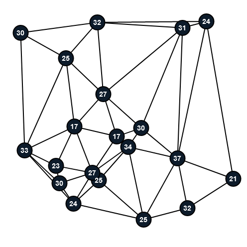
Let be a vertex-weighted graph where is its weight function. In a metaphorical map of , vertex is depicted as polygonal region (country) so that adjacent vertices share a non-trivial contact (boundary). Our optimization goal is to build metaphorical maps such that the area of the region , denoted by , is roughly equal to .
In a metaphorical map , we refer to the points that define its polygonal regions also as vertices. Given two vertices of the metaphorical map, we denote by the vector from to .
2.1 Quality measures for Metaphorical Maps
As mentioned in the introduction, we measure the quality of a metaphorical map by its cartographic accuracy – for this, similarly to the previous work, e.g. [2, 4, 17], we employ the metric normalized cartographic error. The simplicity of the map is measured by the metric polygon complexity, introduced in [8] and applied for the evaluation of metaphorical maps in [17].
Normalized cartographic error.
Consider a vertex of a vertex-weighted graph and its corresponding region in its metaphorical map . The normalized area of region , denoted by , is defined as:
Then, the normalized cartographic error of region is defined as:
| (1) |
Polygon Complexity.
Brinkhoff, Kriegel, Schneider, and Braun [8] defined the complexity of a polygon as a function of three quantities (see also [15] for details), that can be intuitively understood based on an example of a star-shape: (a) the frequency of ’s vibration, denoted by , which specifies how many tips a star-shape has, (b) the amplitude of ’s vibration, denoted by , which specifies how long the tips of a star-shape are and (c) ’s convexity, denoted by , the fraction of the area that is not covered within the smallest enclosing circle. The polygon complexity is then defined as , which maps to values in , with low values meaning low complexity.
In our experiments, we quantify the quality of a map by both the average and the maximum value of normalized cartographic error and polygon complexity over the regions of the map.
2.2 The MS-algorithm
The MS-algorithm [17] is a typical force-directed algorithm that employs several antagonistic forces applied to the vertices of the metaphorical map, that, hopefully, at equilibrium produce a layout with good characteristics, i.e., low normalized cartographic error and low polygon complexity. The algorithm employs three forces (vertex-vertex repulsion, vertex-edge repulsion, and angular-resolution) targeted towards producing metaphorical maps of low polygon complexity and one force (air-pressure) which works towards reducing the cartographic error of the metaphorical map. Here, we only describe the air-pressure force, since our proposed algorithm modifies how this force is applied. The exact definition of the other forces can be found in [15] and in [17].
The normalized air pressure in region , , exerts a force on each bounding edge based on the pressure’s magnitude and the edge’s length in relation to the length of the entire polygonal region boundary ; see [15]for a formal definition of . Thus, the air-pressure force on edge of region was defined as , where is a unit vector perpendicular to directed towards outside of . Force was applied to both endpoints of edge .
The force-directed algorithm is run for number of steps, the value of this parameter is determined experimentally. Notice that the resultant of the forces applied to a vertex of the map, may force it to cross over an edge, and thus, the displacement of each vertex must be limited to prevent this from happening. To achieve that, the MS-algorithm adopted the rules of ImPrEd [22] that ensure the preservation of the planar embedding of the map. It should be also noted that the constant factors employed in each of the described forces have been determined experimentally.
A final note regarding the number of vertices defining each polygonal region. This number fluctuates during the execution of the algorithm in order to allow each region to obtain a more elaborate (or simpler) shape. Let denote the average edge length over all edges in the metaphorical map. Provided that no edge crossings are introduced, the MS-algorithm eliminates vertices of degree 2 that become closer than to their neighbor and it splits in half the edges that get longer than .
Each force-directed algorithm requires for its execution an initial layout. Given a plane vertex-weighted graph , the MS-algorithm constructs an initial metaphorical map by considering the dual of a planar drawing of . The algorithm is designed for internally triangulated graphs. The dual vertices of the inner faces are placed in the barycenters of the triangles representing those faces. The dual edges are drawn as polylines consisting of two segments meeting at a bend-point, which lies in the middle of the corresponding primal edge. Details can be found in [17] and in [15].
3 Our Metaphorical Map Generation Algorithm
In this section, we describe our extension of the MS-algorithm. More specifically, we describe how to revise the air-pressure force utilized in the MS-algorithm by (a) incorporating a stiffness coefficient and (b) by applying a corrective weight coefficient that aims to eliminate narrow passages in the metaphorical map. The constants involved in the calculations of our algorithm are determined experimentally. Finally, we show how the algorithm is adapted in order to accommodate non-triangulated graphs.
The Stiffness of each Map Region.
After examining the output of the MS-algorithm, we observed that some regions had noticeably higher cartographic error than others, leading to the conclusion that some attributes of a region made it less responding to air pressure and, thus, resulted in high cartographic errors. Therefore, for every region we introduce a variable, which we refer to it as stiffness coefficient, that accounts for its stiffness. Let be an internal region and let be its pressure at the -th iteration of the force-directed algorithm. If at iteration region is over-pressured (i.e., ) we increase the region’s stiffness coefficient by a small amount ; if it is under-pressured (i.e., ) we decrease it by , otherwise, it remains unchanged. In addition, we restrict the stiffness coefficient in the range where and . An appropriate value for is determined experimentally.
Given a region , we define the stiffness coefficient of at the -th iteration of the algorithm, denoted by , as:
where
Then, the revised air-pressure force of region on its boundary edge during the -th iteration of the algorithm, , denoted by is defined as
| (2) |
where is the air-pressure force computed at the -th iteration of the MS-algorithm. Note that the “stiffness” attribute is different for each region and demonstrates an adaptive behaviour over time. Employing such adaptive coefficients in force/energy-directed drawing algorithms appears to be uncommon, mainly due to performance issues. However, we note that a similar scheme has been employed in the work of Hu [14] (referred to as adaptive cooling scheme).
We performed a few experiments (see [15] for details) with 20-node graphs in order to determine the parameters of the algorithm, that resulted in the following values: , and . To also account for the size of the input graph, assuming that larger graphs take a longer time to converge to a good metaphorical map, we decided to set the number of iterations to , the value consistent with for .
Improving the Visual Complexity.
When we applied the stiffness coefficients to the regions, we observed that they tended to create long, narrow passages, thereby reducing the visual complexity of the metaphorical map. To mitigate this effect, we introduce a new corrective weight coefficient for the pressure forces exerted on each region’s vertices, while keeping the total pressure of the region constant. These weight coefficients redistribute pressure so that vertices in narrow passages receive a larger share of the force, whereas vertices in wider parts of the region receive less. Before defining the weight coefficient, we introduce some auxiliary notation:
-
Let be a metaphorical map, and let denote the radius of a circle whose area equals the total area of . We refer to as the ideal radius of .
-
Let be a region of , let be one of its vertices and let be an edge of that is not adjacent to . Further, let be the point of that is closest to . The Euclidean distance of to , denoted by , is simply the Euclidean distance from to point . We also define the polygonal distance of vertex to edge , denoted by , as the length of the shortest path when moving from to on the boundary of .
Intuitively, an edge is sufficiently “opposite” to a vertex if it is close to it and, at the same time, it belongs to the opposite side of a narrow passage. For each vertex of region , we want to identify the edge of that is the closest out of those opposite to it. In order to avoid selecting edges that are collinear with , we consider only edges for which it holds that and, out of those, we select the edge of smallest Euclidean distance to . We refer to this edge as the pairing edge of and we denote it by . Further, we denote the Euclidean distance from to by .
Consider the metaphorical map . We introduce a scale factor based on the ideal radius . We regard as the minimum “acceptable” passage width and, hence, we define the quantity which assumes values greater than 1 when is very close to its pairing edge .
We now define the corrective coefficient that will be applied to the air-pressure forces at each vertex of region of the metaphorical map as:
Hence:
-
If , i.e., marginally does not participate in a narrow passage, then .
-
If , then which grows logarithmically once exceeds 1.
-
If , then which remains below 1 but varies smoothly as decreases.
Let and be the endpoints of edge of region and let be a unit vector perpendicular to directed towards the exterior of . Recall that, the air-pressure force on is defined as , where is the stiffness coefficient in the current iteration. Since the air-pressure force is exerted on both endpoints of , the total air-pressure force on is and the total air-pressure force of region is .
The new air-pressure force, employing the above introduced corrective coefficient , on edge is now defined as
Therefore, the total air-pressure force applied to region equals to . So, we have that:
, and thus, the total air-pressure force on region remains unchanged.
3.1 Dealing with non-Triangulated Graphs
In this section, we discuss how to create metaphorical maps for biconnected, non-triangulated plane graphs. Mchedlidze and Shnorr [17] focused on the case of internally triangulated graphs. However, their algorithm was, in principle, able to also deal with non-triangulated graphs provided that, in the initial layout of the given graph, the barycenter visibility property is satisfied, that is, the barycenter of each non-triangulated face is located within that face and all vertices of the face are visible from the barycenter, that is, the open segment that connects the barycenter and any vertex of the face does not cross the boundary of the face.
We proceed to establish the barycenter visibility property as follows. We internally triangulate the graph by creating a new auxiliary vertex for each non-triangulated inner face and connecting it to every vertex of the face. The use of auxiliary vertices for mesh generation, often called Steiner points, is a common technique to transform general grids into high-quality triangulations (see [5, 19]). Let be the resulting internally triangulated graph where and are the sets of auxiliary vertices and the extra edges used in the triangulation, respectively. We apply on Tutte’s barycentric embedding algorithm [26] that fixes the outerface on a circle and places every inner vertex on the barycenter of its neighbors, resulting in a planar straight line layout ; refer to Fig.˜2.(a-b) We finish by removing the auxiliary vertices and their adjacent edges from ; refer to Fig.˜2.(c). It is trivial to see that the derived layout satisfies the barycenter visibility property. Indeed, the auxiliary vertex of each non-triangulated face is placed at the barycenter of its neighbors, that is, the vertices of . Therefore, in the constructed planar drawing, face has its barycenter lying inside it. Moreover, the fact that the auxiliary edges inside do not cross the boundary of , ensures the visibility between the barycenter of and all of ’s vertices.


After ensuring that the barycenter of every inner face lies within its boundary, we are in a position to obtain an initial metaphorical map by using the transformation deployed in the MS-algorithm; refer to Section 2.2 and Fig.˜2.(d). Note that this transformation leads to points in the metaphorical maps where more than three regions meet. Recall that in our definition of the metaphorical map, only the non-degenerate contacts represent adjacencies, therefore the maps constructed this way still represent exactly the adjacencies present in the given graph.
Metaphorical maps with holes.
By visually inspecting the maps created with the above method, we noticed that the large faces (in the initial graph) which result in multiple point contacts (in the map) appear to be quite cluttered; refer to Fig.˜2.(d) and Fig.˜3.(a). Therefore, we propose an alternative method that treats large faces as holes; Refer to Fig.˜2.(e). Practically, obtaining such maps is very simple – we can just consider the graph obtained after the introduction of the auxiliary vertices, transform it to a map, as suggested in the MS-algorithm , and treat regions corresponding to the auxiliary vertices as holes. When applying forces to the map vertices, we can treat holes in exactly the same way we treat other regions. However, since the holes do not have a target weight, we have the flexibility to assign those weights with the goal to improve the appearance of the overall map. Our intuition is that the more regions are adjacent to a hole, and the heavier those regions are, the bigger the hole needs to be. After some experimentation, we found that the following function for assigning weights to holes produces reasonably good results, however, with further testing better functions may arise:
| (3) |
Note that, we do not prioritize minimizing the normalized cartographic error within holes, as they do not represent regions. However, it is important that holes remain visually simple to preserve the clarity of adjacencies. To allow adjacent regions the flexibility to expand naturally, we do not apply stiffness coefficients to holes. Nonetheless, we do apply the corrective weight coefficients of the pressure forces to maintain overall layout stability.


4 Experimental Evaluation
In our experimental evaluation we aim to answer the following research questions:
-
1.
What is the performance of our algorithm compared to the performance of the MS-algorithm based on the quality metrics of normalized cartographic error and polygon complexity? Does the difference in performance depend on the input characteristics such as number of vertices, nesting ratio or weight ratio (refer to Section 4 for the definitions)?
-
2.
Is there a trade-off between cartographic error and polygon complexity? How do we control it?
-
3.
Does the initial metaphorical map have an effect on the quality of the final one?
-
4.
Is the handling of non-triangulated biconnected graphs satisfactory?
-
5.
Is the proposed algorithm practical? Does its running time scale well with the size of the input graph?
The analysis of question 5 can be found in [15].
The Graph Test Data.
For the generation of test data, we followed the approach of [17] (described in detail in Algorithm 5.1 of [21] with a uniform distribution). The authors of [17] generate planar straight-line drawings based on the Delaunay triangulation of a random point set. A fraction of the points, called nesting ratio, is placed within the triangles of the initial Delaunay triangulation. It was experimentally verified in [17] that the nesting ratio has an effect on the algorithm’s performance, therefore, we also included it in our analysis. For every vertex, we generate a weight using a uniform distribution with different weight ratios of maximum to minimum weight. The above described procedure is augmented to generate non-triangulated plane graphs as follows. Following the generation of an internally triangulated plane graph, we remove a number of randomly selected internal edges in order to create non-triangulated plane graphs. We denote the ratio of removed to initial internal edges by . Note that an edge is only removed if the graph remains biconnected.
Comparison to the MS-algorithm.
For the comparison of the performance of our algorithm (NEW-algorithm) against MS-algorithm, we examined how three parameters – the nesting ratio (see Fig.˜4), the weight ratio (see Fig.˜5), and the total number of nodes (see Fig.˜6)–influence both algorithms. To this end, we conducted three experiments:
-
1.
Varying nesting ratio. For each value of , we generated 50 graphs with nodes and weight ratio .
-
2.
Varying weight ratio. For each , we generated 50 graphs with nodes and nesting ratio .
-
3.
Varying number of nodes. For each , we generated 50 graphs with nesting ratio and weight ratio and we let the algorithms run for iterations.
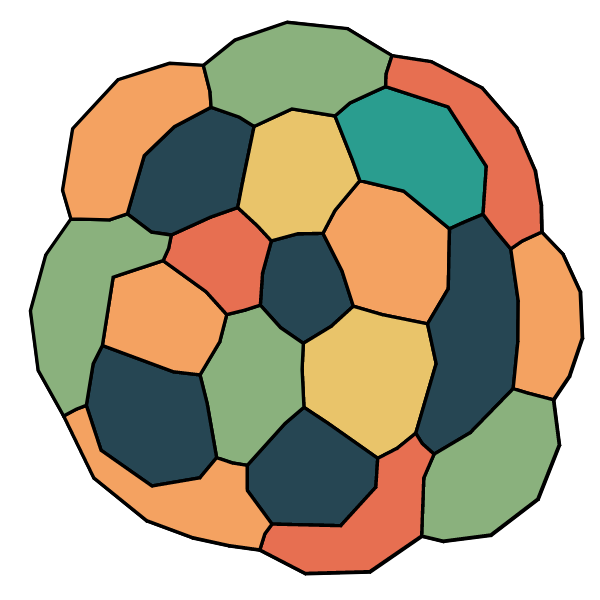
The results of every comparison follow a similar trend. Our algorithm achieves average cartographic error close to zero at the cost of a slightly higher polygon complexity. In all of our experiments (1450 in total), the recorded average normalized cartographic error (for each metaphorical map created) was in the range . In comparison, the same metric for MS-algorithm is in the range . The price we paid was a small increase in the average polygon complexity. The highest observed increase in average polygon complexity over all the maps was and was observed for , where the maximum value of average polygon complexity was , well below the value where polygons are considered to be complex [8]. The maps in our experiment that correspond to this maximum value of increase in the average polygon complexity are shown in Fig.˜7.(a-b). We observe that indeed our map’s regions are longer and, sometimes, narrower. However, in the case of smaller (or “simpler”) graphs, this increase in complexity is hardly noticeable, see e.g. Fig.˜7.(c-d). Regarding the properties of the graphs, all three parameters (nesting ratio, weight ratio, and the number of vertices) affect the polygon complexity of our produced maps.


Cartographic error and polygon complexity trade-off.
The cost we pay for achieving average cartographic error close to zero is a small increase in the average polygon complexity. Given that our algorithm is identical to the MS-algorithm for stiffness (without the application of the corrective weight coefficients on the pressure forces), we evaluated our algorithm for several values of (see Fig.˜8). We observed that while the average and maximum normalized cartographic error remain nearly identical for and , the algorithm performs better at in terms of both average and maximum polygon complexity. Based on these observations, we set in our algorithm. This value achieves very small cartographic error while maintaining acceptable polygon complexity. Moreover, increasing beyond 8 does not lead to meaningful improvements in either evaluation metric.
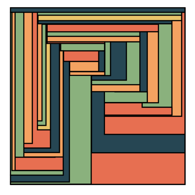
Fig.˜9 shows a “heat-map” style coloring of the regions of metaphorical maps of the same graph for MS-algorithm (Fig.˜9.(a)) and our algorithm for (Fig.˜9.(b)-(c)), demonstrating the effect of the introduction of the stiffness coefficient. These experiments reveal a monotonic decrease in the maximum/average cartographic error and a monotonic increase in maximum/average polygon complexity based on the value of .


Non-Triangulated Graphs.
We tested our algorithm for graphs with ratio of removed edges (Fig.˜10 and 11). For each value of , we conducted experiments on fifty graphs, each with forty nodes, a nesting ratio of zero, and a weight ratio of five. We let the algorithm run for iterations. Recall that hole region weights were assigned according to Equation 3. Normalized cartographic error and polygon complexity were measured only for non-hole regions.
We observed that increasing the parameter rem (i.e., the fraction of removed edges) led to a slight increase across all four evaluation metrics (Fig.˜10). This can be explained by the fact that the increasing number of missing edges creates more complex patterns of adjacency, i.e. holes behave as nodes of high degree.
We also observed that holes can have narrow passages; refer to Fig.˜11.(c)-(d), which possibly can also be explained by the relatively high number of regions adjacent to a hole. We anticipate that this effect can be mitigated by using a different hole weight function and by re-engineering the applied forces.


The effect of the initial drawing.
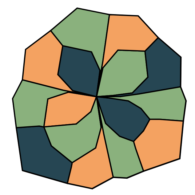
Given that we managed to, effectively, get the average cartographic error down to zero, we did not study the effect of the initial metaphorical map used by our algorithm on the cartographic error. Instead, we focused on the polygon complexity and we examined the effect of having an initial map with good average cartographic error. As such good initial maps we considered the maps produced by the algorithm in [3] (referred to as octagonal map) which produces rectangular maps with at most 8 corners and of average cartographic error close to zero. We observed that, when using octagonal maps as initial layout, no consistent improvement was observed while the produced maps appeared to have long and skinny regions. Moreover, when the number of vertices becomes larger the metaphorical maps become harder to read due to their long, skinny, and circular shaped regions. See Fig.˜12.(a-d) and Fig.˜12.(e-h) for sample metaphorical maps of 20 and 40 regions, respectively. Finally, it is noted that our algorithm also required a larger number of iterations (about double) when initialized with such maps in order to converge to its final metaphorical map solution.


5 Conclusion
In this work we have proposed an improvement of MS-algorithm [17] that produces metaphorical maps of vertex-weighted graphs and presented a detailed experimental evaluation of the newly proposed algorithm. Our goal was to close the gap between the metaphorical maps with perfect cartographic accuracy [2, 16, 24] that despite using a few corners per polygonal region can look quite complex and the simple-looking metaphorical maps produced by MS-algorithm with cartographic error up to 30%. Our experiments showed that we can achieve cartographic error close to zero, by paying a small price for the polygon complexity. Our algorithm achieves this improvement by using the notion of region stiffness that adapts as the force-directed simulation runs. We have seen that the maximum value of this stiffness determines the interplay between the cartographic error and polygon complexity.
To quantify the complexity of the maps, we applied the quality metric introduced in [8], who presented examples of geographic maps showing that this metric corresponds to the human intuition of map complexity. Our experiments with metaphorical maps do not contradict this intuition. However, we believe that whether this function is indeed appropriate for qualifying the human intuition of the metaphorical maps complexity has to be investigated in a user study.
We conjecture that the performance of the algorithm for non-triangulated graphs can be further improved by considering different hole weight functions and by engineering the forces to avoid narrow passages. Finally, it is also interesting to compare the quality of the maps for non-triangulated graphs with and without holes. We defer these investigations to the extended version of this work.
References
- [1] Muhammad Jawaherul Alam. Contact representations of graphs in 2D and 3D. Doctoral thesis, The University of Arizona, 2015. URL: https://www.proquest.com/openview/5bf2b2dc7f21bf9f8759bdc89632b50b/1?pq-origsite=gscholar&cbl=18750.
- [2] Muhammad Jawaherul Alam, Therese Biedl, Stefan Felsner, Andreas Gerasch, Michael Kaufmann, and Stephen G. Kobourov. Linear-time algorithms for hole-free rectilinear proportional contact graph representations. Algorithmica, 67(1):3–22, 2013. doi:10.1007/S00453-013-9764-5.
- [3] Muhammad Jawaherul Alam, Therese Biedl, Stefan Felsner, Michael Kaufmann, Stephen G. Kobourov, and Torsten Ueckerdt. Computing cartograms with optimal complexity. Discrete & Computational Geometry, 50(3):784–810, 2013. doi:10.1007/s00454-013-9521-1.
- [4] Muhammad Jawaherul Alam, Stephen G. Kobourov, and Sankar Veeramoni. Quantitative measures for cartogram generation techniques. Comput. Graph. Forum, 34(3):351–360, 2015. doi:10.1111/cgf.12647.
- [5] Marshall Bern and David Eppstein. Mesh Generation and Optimal Triangulation, pages 47–123. World Scientific Publishing Co Pte Ltd, 1995. doi:10.1142/9789812831699_0003.
- [6] Robert P. Biuk-Aghai, Patrick Cheong-Iao Pang, and Bin Pang. Map-like visualisations vs. treemaps: an experimental comparison. In Robert P. Biuk-Aghai, Jie Li, and Shigeo Takahashi, editors, Proceedings of the 10th International Symposium on Visual Information Communication and Interaction, VINCI 2017, Bangkok, Thailand, August 14-16, 2017, pages 113–120. ACM, 2017. doi:10.1145/3105971.3105976.
- [7] I. Bortins, S. Demers, and K. Clarke. Cartogram types, 2002.
- [8] Thomas Brinkhoff, Hans-Peter Kriegel, Ralf Schneider, and A. Braun. Measuring the complexity of polygonal objects. In Patrick Bergougnoux, Kia Makki, and Niki Pissinou, editors, Proceedings of the 3rd ACM International Workshop on Advances in Geographic Information Systems, Baltimore, Maryland, USA, December 1-2, 1995, in conjunction with CIKM 1995, page 109. ACM, 1995.
- [9] Rafael G. Cano, Kevin Buchin, Thom Castermans, Astrid Pieterse, Willem Sonke, and Bettina Speckmann. Mosaic drawings and cartograms. Comput. Graph. Forum, 34(3):361–370, 2015. doi:10.1111/cgf.12648.
- [10] Prabu David. Seeing is believing: Comparative performance of the pie and the bar. Newspaper Research Journal, 17(1-2):89–104, 1996. doi:10.1177/073953299601700109.
- [11] Mark de Berg, Elena Mumford, and Bettina Speckmann. On rectilinear duals for vertex-weighted plane graphs. Discret. Math., 309(7):1794–1812, 2009. doi:10.1016/j.disc.2007.12.087.
- [12] Danny Dorling. Area cartograms: their use and creation. University of East Anglia: Environmental Publications, 59, 1996.
- [13] Marius Hogräfer, Magnus Heitzler, and Hans-Jörg Schulz. The state of the art in map-like visualization. Comput. Graph. Forum, 39(3):647–674, 2020. doi:10.1111/cgf.14031.
- [14] Yifan Hu. Efficient and high quality force-directed graph drawing. Mathematica Journal, 10:37–71, January 2005.
- [15] Eleni Katsanou, Tamara Mchedlidze, Antonios Symvonis, and Thanos Tolias. An algorithm for accurate and simple-looking metaphorical maps. Tech. Report arXiv:2508.19810, Cornell University, 2025. doi:10.48550/arXiv.2508.19810.
- [16] Linda Kleist. Drawing planar graphs with prescribed face areas. J. Comput. Geom., 9(1):290–311, 2018. doi:10.20382/jocg.v9i1a9.
- [17] Tamara Mchedlidze and Christian Schnorr. Metaphoric Maps for Dynamic Vertex-weighted Graphs. In Marco Agus, Wolfgang Aigner, and Thomas Hoellt, editors, EuroVis 2022 - Short Papers. The Eurographics Association, 2022. doi:10.2312/evs.20221090.
- [18] Sabrina Nusrat and Stephen G. Kobourov. The state of the art in cartograms. Comput. Graph. Forum, 35(3):619–642, 2016. doi:10.1111/cgf.12932.
- [19] Steven J. Owen. A survey of unstructured mesh generation technology. In 7th International Meshing Roundtable, 1998.
- [20] Bahador Saket, Carlos Scheidegger, and Stephen G. Kobourov. Comparing node-link and node-link-group visualizations from an enjoyment perspective. Comput. Graph. Forum, 35(3):41–50, 2016. doi:10.1111/cgf.12880.
- [21] C. Schnorr. Visualizing dynamic clustered data using areaproportional maps. Master’s thesis, Karlsruhe Institute of Technology, 2020. URL: https://github.com/jenox/Master-Thesis.
- [22] Paolo Simonetto, Daniel Archambault, David Auber, and Romain Bourqui. Impred: An improved force-directed algorithm that prevents nodes from crossing edges. Comput. Graph. Forum, 30(3):1071–1080, 2011. doi:10.1111/j.1467-8659.2011.01956.x.
- [23] Roberto Tamassia, editor. Handbook on Graph Drawing and Visualization. Chapman and Hall/CRC, 2013.
- [24] Carsten Thomassen. Plane cubic graphs with prescribed face areas. Comb. Probab. Comput., 1:371–381, 1992. doi:10.1017/S0963548300000407.
- [25] Waldo Tobler. Thirty five years of computer cartograms. An. of the Assoc. of American Geographers, 94(1):58–73, 2004. doi:10.1111/j.1467-8306.2004.09401004.x.
- [26] William Thomas Tutte. How to draw a graph. Proceedings of the London Mathematical Society, 3(1):743–767, 1963.
- [27] Han-Ming Wu, ShengLi Tzeng, and Chun-houh Chen. Matrix Visualization, pages 681–708. Springer Berlin Heidelberg, Berlin, Heidelberg, 2008. doi:10.1007/978-3-540-33037-0_26.
- [28] yWorks GmbH. yfiles for html. https://www.yworks.com/products/yfiles-for-html, 2025. Software library.