Circle-Segment Intersection Queries
in Connected Geometric Graphs
 Yannick Bosch
Sabine Storandt
Yannick Bosch
Sabine Storandt
Abstract
In this paper, we study the problem of efficiently reporting all intersections between a given set of line segments in the plane and a query circle, focusing on the case where the segments form the edges of a connected geometric graph. While previous data structures for circle-segment intersection queries on general segment sets incur high space or query time costs, we exploit the connectivity of the input to obtain significantly improved performance. In fact, we propose a new circle-segment intersection data structure that can be constructed in time and space on connected graphs with edges and edge crossings. It answers intersection queries in time, where denotes the output size. Our method relies on the construction of efficient circle-graph intersection oracles as well as a novel linear-time algorithm to partition the edges of the graph into balanced, connected components, which might be of independent interest. In a proof-of-concept experimental study on real-world road networks, we show that our novel data structure also performs well in practice. Even on networks with millions of edges, the construction time is within minutes and queries are answered in a few milliseconds.
Keywords and phrases:
Intersection data structure, Graph partitioning, Dobkin-Kirkpatrick hierarchyCopyright and License:
![[Uncaptioned image]](x1.png) © Peyman Afshani, Yannick Bosch, and Sabine Storandt; licensed under Creative Commons License CC-BY 4.0
© Peyman Afshani, Yannick Bosch, and Sabine Storandt; licensed under Creative Commons License CC-BY 4.0
2012 ACM Subject Classification:
Theory of computation Computational geometry ; Theory of computation Data structures design and analysisAcknowledgements:
This work was initiated at Dagstuhl Seminar 25191 “Adaptive and Scalable Data Structures” (2025-05-04 – 2025-05-09) https://www.dagstuhl.de/25191. We thank Schloss Dagstuhl -– Leibniz-Zentrum für Informatik for their support.Editors:
Ho-Lin Chen, Wing-Kai Hon, and Meng-Tsung TsaiSeries and Publisher:
 Leibniz International Proceedings in Informatics, Schloss Dagstuhl – Leibniz-Zentrum für Informatik
1 Introduction
Given a set of geometric objects and a query object , reporting the intersections of with elements in is a fundamental task in computational geometry. In this work, we focus on the scenario where is a set of segments in the Euclidean plane, and is a query circle whose center and radius is revealed at query time. The goal is to preprocess into a data structure that allows to report circle-segment intersections efficiently.
Notably, there are two different types of intersections that can occur between a segment , specified by its endpoints , and a query circle , specified by its center and its radius :
-
Type-(i) intersection: This intersection occurs if and , that is, one endpoint of is inside the query circle and the other one outside of it.
-
Type-(ii) intersection: This intersection occurs if and but , that is, both endpoints of are outside of the query circle but part of the segment is inside the circle.
Both intersection types are visualized in Figure 1.
Closely related to circle queries are disk queries, where segments fully contained within the disk need to be reported as well. So for disk queries, if a data structure identifies the set of segment endpoints that are contained in the disk, one can batch report all incident segments, as those are either completely contained in the disk or have a type(i)-intersection with its boundary circle. Thus, circle queries are somewhat more intricate than disk queries, as here this batch reporting cannot be applied if output-sensitive query times are desired. In [16], different data structures for each intersection type were proposed to cater for circle-segment and disk-segment intersection queries on a given set of input segments. For fixed radius, after an construction phase, a data structure of size allows to answer circle or disk queries in time or , where denotes the output size. For variable radius, a data structure of size was shown to answer queries in for . Significantly improved query times of are also possible but at the cost of a much higher space consumption of . Other trade-offs between data structure size and query time can be obtained as well. For example, the query times for the fixed radius case can be matched for the variable radius scenario using a data structure of size . In all these scenarios, the data structure for detecting type-(ii) intersections dominates the space consumption and the query time.
In this paper, we consider a special case of the circle- or disk-segment intersection problem, in which the segments in are the edges of a connected geometric graph . There are numerous applications of circle-edge or disk-edge intersection queries:
-
Nearest Edges. Given a geometric graph and a query point , identifying the edges of that are within distance of is equivalent to a disk query on the edge segment set. This query type is useful, for example, for the construction of segment proximity graphs [1] or in edge facility location problems [20].
-
Motion planning for circular robots. Obstacle collision avoidance for robots that have to navigate a mesh or are supposed to sweep a given polygon (e.g. a floor plan) requires to detect whether the robot boundary intersects any obstacle [21]. For circular robots, a circle-segment reporting data structure can be leveraged to detect collisions.
-
Map matching. Let be a road network where edge costs describe travel times. A map matching query is specified by a sequence of measurements (usually obtained via GPS) where denotes the measured position, the error radius (stemming from measurement imprecision) and the time stamp of the measurement. The goal is to match each position to a location in that is within distance of such that can be reached from on a path in with travel time at most . It was proven in [8] that a feasible map matching solution can be fully characterized by the intersection points of the circles with edges in , and an efficient algorithm was proposed that leverages a circle-segment data structure.
Some example queries on a city road network are visualized in Figure 2.
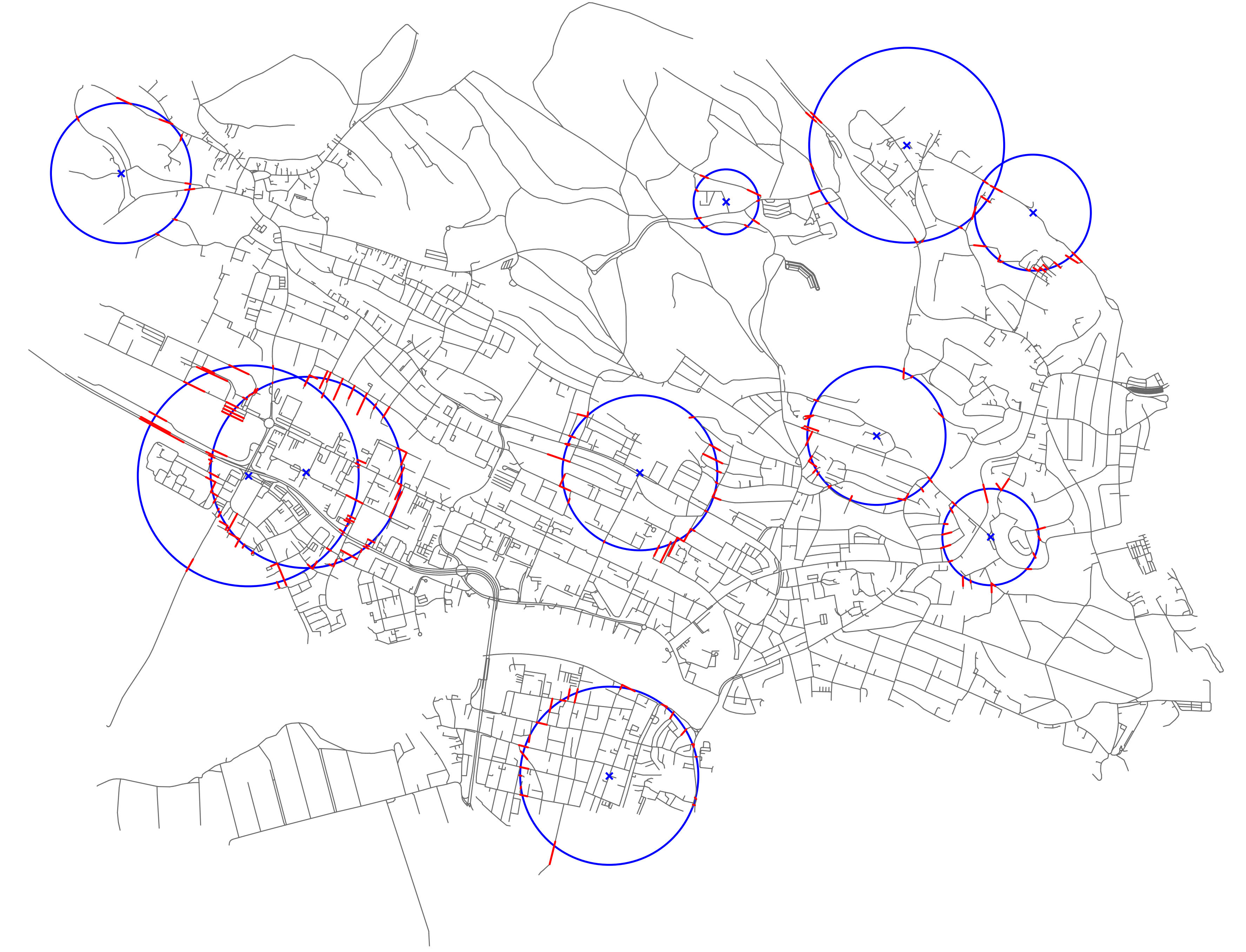
We show that we can utilize the connectivity of to significantly improve the construction time, the space consumption, and the query times of circle- or disk-segment intersection data structures in theory and practice.
1.1 Related Work
There are interesting special cases of the circle-segment or disk-segment intersection problem, which have been studied in the literature:
-
If all input segments have length zero, the input is simply a set of points. Thus, the problem degenerates into reporting all points on the boundary of a query circle or inside a query disk. The latter is also known as the disk range searching problem. Disk range searching in can be transformed into halfspace range searching in , for which a data structure of size allows to answer queries in [5].
-
If the circle has a radius of zero, it degenerates into a point. Then, the circle/disk query asks for the segments that contain the query point, also known as segment stabbing problem. If the segments are assumed to be disjoint, queries can be answered in after a preprocessing phase that produces a data structure of linear size [12].
For the general case, the data structures for type-(i) and type-(ii) circle/disk-segment intersection described in [16] are the state-of-the-art. For variable radius, first a partition tree on the segment endpoints is constructed [19] after projecting the points to . Here, the point set is recursively partitioned using simplices, such that in the resulting hierarchical tree, the number of points in each child partition is a constant fraction of the number of points in the parent partition and only a bounded number of children intersect a query object at each level. To only retrieve the intersecting segments with an endpoint inside the circle, the data structure is augmented such that halfplane composition queries can be answered. Also type-(ii) intersections can be identified with the help of halfplane query compositions. This gives rise to a data structure of size with query times in for , as well as the other trade-offs mentioned in the introduction.
For fixed radius, type-(i) and type-(ii) intersections are computed with two different data structures. For type-(i), first a stabbing path is computed on the segment endpoints. This path is guaranteed to intersect a given query circle at most times. On this path, a tree data structure is constructed, which is augmented with a halfplane query data structure at each node. Using geometric transformations and dualization, this allows to identify the segments with an endpoint outside and an endpoint inside the query circle. For type-(ii) intersections, a reduction to triangle stabbing is described and proper data structures for this use case are leveraged. In [8], the data structure for circle-segment queries with fixed radius from [16] was refined and improved for the case in which the input segments form a path to show improved theoretical running times for map matching. However, for practical implementation, an AABB tree is used in [8], as the nested data structures described in [16] are rather intricate and expensive to construct. The AABB tree, available as a ready-to-use implementation in CGAL, is a hierarchical data structure in which each node corresponds to an axis-aligned bounding box (AABB) that encapsulates the set of geometric primitives associated with its descendant leaf nodes (in this case, the input segments). While often fast in practice, it cannot guarantee output-sensitive query times as the bounding box of a segment set might intersect a given geometric query object (as a circle) while none of the contained segments actually have an intersection with .
In [4], the segment-circle intersection problem was studied, in which the roles of the input and the query are switched compared to our setting. Here, the input is a set of circles and the query object is a segment. It was shown that the circles can be preprocessed into a data structure of size such that queries can be answered in where denotes the output size. For disks, the query time reduces to .
There are also other contexts in which the connectivity structure of the input segments plays a crucial role. For example, in [3], the input is a set of segments and the goal is to report the connected components that intersect a given query segment. In [6], it was shown that intersections between two sets of line segments can be computed much faster if each of the two sets is connected.
1.2 Contribution
We propose a new data structure for circle-segment or disk-segment intersection queries on connected planar graphs with edges, which can be constructed using time and space, and answers queries with output size in time . This is a significant improvement over the general case, where a data structure of (near-)linear size yields query times in for . Thus, especially for queries with small output size, our query time is vastly superior. If the input graph is non-planar and there are crossings among the segments, the construction time and the space consumption increase to but the query time stays the same. At the heart of our data structure lies a scheme which partitions the edges of the connected input graph, such that the resulting partitions have balanced size and each still form connected components. We show that such a partitioning can be computed in time . Applying this result recursively allows us to efficiently construct an edge partition tree111We remark that despite the similar name our data structure differs substantially from the partition tree concept for point sets described in [19]. of logarithmic depth. We then equip each such edge partition with an oracle that decides whether for a given query circle there is some edge in the set that intersects . Based on this oracle, the tree can be traversed efficiently on query time.
We also carefully describe how to implement the proposed data structure and demonstrate its usefulness in a proof-of-concept evaluation on different road networks. While road networks are non-planar, the number of crossings between the edges is typically in [15] and thus we expect our data structure to perform well. This is confirmed in the experiments where we observe fast construction times even on large networks, and improved query times over the AABB tree implementation provided by CGAL.
2 Preliminaries
Throughout the paper, we assume to be given a connected geometric graph as input. The graph nodes are points in and each edge forms a straight-line segment between its endpoints. The number of pairwise crossings between edge segments is denoted by . Here, an edge crosses another edge if their intersection contains a point that is not an endpoint of both edges. We assume that no pair of edges intersects in more than one point. Connectivity of implies that there is a simple path between any pair of nodes in the graph, formed by sequence of edges from . Thus, connectivity solely relies on the graph structure. This is in contrast to the notion of connected arrangement of segments, in which the set of points induced by the segments needs to be connected [3]. While in a connected geometric graph the edge segment arrangement is also connected, the reverse is not necessarily true (consider a set of segments which all pairwise cross). However, in a planar graph embedding, where we have , these two definitions coincide.
3 An Improved Data Structure for Connected Geometric Graphs
In this section, we introduce our new data structure that leverages the connectivity of the input graph to answer circle-edge and disk-edge intersection queries more efficiently.
In all approaches presented in [16] for the general case, the primary data structure is constructed by only considering the endpoints of the input segments. Either a spanning path with bounded stabbing number is computed on that point set or a partition tree is constructed on the (transformed) endpoints. Thus, any connectivity information is immediately lost. The original segments are only indexed in secondary or even tertiary data structures which are queried individually if the respective point sets fulfill certain requirements.
In contrast, our data structure construction is driven by the edges of . In Section 3.1, we prove that the edges of a connected graph can be partitioned into two subsets, such that each partition remains connected and the partition sizes are a constant fraction of the total number of edges. The respective partitioning can be computed in linear time. By applying this method recursively, we obtain an edge partition tree of logarithmic depth in which the leaves correspond to individual segments. In Section 3.2, we describe how to equip each node of the edge partition tree with an oracle that efficiently decides whether a given query circle has a type-(i) or type-(ii) intersection with some edge in the connected subgraph associated with the tree node. This allows to traverse the tree in DFS-order for query answering, only following paths for which the oracle answer is positive. More details on the query answering procedure are given in Section 3.3.
3.1 Balanced Connected Graph Partitioning
In the construction of our intersection search data structure, we follow the well-established paradigm of recursively dividing our problem into smaller subproblems until they reach a tractable size. To accomplish this while also being able to utilize the connectivity of the input graph, we require an algorithm that partitions the edge set of the input graph such that the connectivity property is maintained in each partition. Existing geometric partitioning methods (for example, median- or grid-based) are oblivious to the connectivity structure and thus are not guaranteed to produce the desired result. The method we propose does the opposite as it completely ignores all geometric information and instead operates only on the abstract graph. It is thus also applicable to non-geometric graphs. Edge partitioning has previously been studied in the context of distributed graph algorithms and parallelization [9, 22]. However, there the goal is to minimize communication cost introduced by the partitioning or to minimize node duplication (which turns out to be NP-hard). However, our focus is on balanced partitioning into connected components. In the remainder of this subsection, we prove the following central theorem.
Theorem 1.
Given a connected graph induced by the edge set of size , there is an -time algorithm that partitions into and such that:
-
,
-
is connected for ,
-
for .
We now describe the partitioning algorithm in detail and then prove its correctness to establish the theorem. The algorithm starts by constructing a spanning tree of via a DFS run from an arbitrarily selected source node . Let denote the nodes of the subtree of the DFS-tree that is rooted at node . The following observation sketches how we can use the notion of to achieve our goal of connected edge partitioning.
Observation 2.
Let be the set of edges in that are incident to nodes in . The graphs induced by the edge partitions and are each connected.
But we still need to take care of the size bound for each partition. Thus, we would like to efficiently compute the function that assigns to each node the number of edges incident to the nodes in . Initially, we set for all nodes . We then consider the nodes one after the other using a post-order traversal of the DFS-tree and update the -values of the current node as well as its parent node in the DFS-tree. We will maintain the invariant that at the moment that is processed, all -values are less than . This condition is clearly fulfilled after the initialization phase.
Let us now consider the algorithm steps for processing a node . As we use post-order traversal of the DFS-tree, we know that is the last node to be processed in . We first check whether , where denotes the degree of in . If that is the case, we add to and then proceed to add the new value to where . If we still have , we are done with and proceed to the next node in the post-traversal order. Clearly, our invariant is maintained in this case. Otherwise, if , we also know that , as our invariant guaranteed that was smaller than prior to processing and we only updated the parent of as held as well. Accordingly, with be the children of that were already processed up to this point (and thus contributed to ), we set and . The resulting partitions are each connected, as contains all edges induced by and additionally only edges with at least one endpoint in , while contains all induced edges of and additionally only edges with at least one endpoint in this node set.
If, however, , we know that edges incident to nodes in already suffice to form . If additionally , we simply return and . If the degree of is too large to include all of its incident edges in , we only use many, giving priority to edges with . Note that there are less than such prioritized edges, as otherwise would have been equal to or larger than already, which would contradict our invariant. Therefore, we are sure to include all edges induced by and therefore, again, guarantee connectivity of the resulting partitions.
Thus, the described algorithm reliably produces edge partitions and , whose induced graphs are connected. However, we did not take double counting of the edges into consideration so far. An edge with might contribute twice to , as both and are part of the sum. Therefore, the -values might overestimate the real number of edges in the respective subtree by a factor of up to 2. Thus, we can so far only guarantee a weaker size bound than the one promised in Theorem 1.
Lemma 3.
The partitioning algorithm runs in and produces connected edge partitions and each of which has a size of at most .
Proof.
The DFS run takes time. In the post-order traversal, each node is processed at most once, and the processing step takes constant time if we do not return the result after this step, and at most linear time for the step after which the algorithm terminates. Therefore, the total processing time is in . By construction, the returned partitions and are connected and the estimated size of is between and . But as some edges might have contributed twice to this estimation, it follows that we actually have . With , it follows that . We remark that this size bound is already sufficient for our goal of constructing a partition tree on the edge set with logarithmic depth, and the simplicity of the algorithm also makes it very suitable for practical implementation. However, we can ensure a better partition size balance within the same asymptotic running time as follows. To avoid double counting, we first refine the DFS-tree to a binary tree by introducing for all nodes with more than two children a complete binary tree rooted at with the children forming the tree leaves. By the property of complete binary trees the total number of nodes and edges in the DFS-tree is at most doubled by this step. Moreover, we compute a lowest-common-ancestor (LCA) data structure on the refined DFS-tree rooted at . Such a data structure can be constructed on trees in linear time and it answers LCA queries for node pairs in [7]. We then use the processing algorithm described above with two modifications: When processing a dummy node introduced in the binary tree refinement step, we assume its degree to be zero. When processing a real node , we still add to , but we additionally iterate over its neighbors with and decrement by one if comes later in the processing order than . We refer to this algorithm as improved partitioning algorithm.
Lemma 4.
The improved partitioning algorithm runs in and produces connected edge partitions and each of which has a size of at most .
Proof.
The binary refinement step and the LCA data structure construction both run in linear time. The processing of now takes , as the LCA data structure needs to be queried for each neighbor. Summed over all nodes, the degrees add up to and therefore the overall running time is still linear.
Next, we argue that after was processed and the algorithm did not yet terminate, we have . The proof uses induction over the nodes in post-order traversal. The first node to be processed is a leaf of the DFS-tree and thus . If , we set and therefore we also have . Let us now assume that the induction hypothesis applies to the first nodes in the post-order traversal and consider node number , which we refer to as . For each child of in , we know that was processed prior to and therefore . If has only a single child , we have right before is processed. This is true because propagates its -value to its parent and for all with we have an comes later in the processing order than . Now adding to , we get . If has two children and , then for all edges with and we have and thus was decremented by 1 for each such edge. It follows that we have right before is processed. As the last term is exactly the number of edges that are counted twice, once in and once in , we get again after adding to . Therefore, if we terminate while processing node because , we are now indeed guaranteed that contains the promised number of edges.
But we might also terminate after processing some node as the -value of its parent node exceeded the threshold after adding . We first observe that this can only happen if is the last child of to be processed. If it is the first child, then holds prior to the processing of . The value is initialized with zero, but might even become negative it is the LCA of the endpoints of an edge that connects nodes in the respective subtree. Therefore, after the processing of , we have . And as for the propagation step to happen, it follows as well. If is the last child to be processed, we know that by the same argumentation as above. Thus, there is no double counting occurring in this scenario and it is safe to construct as described in the original partitioning algorithm. We conclude that the improved partitioning algorithm takes linear time and guarantees for .
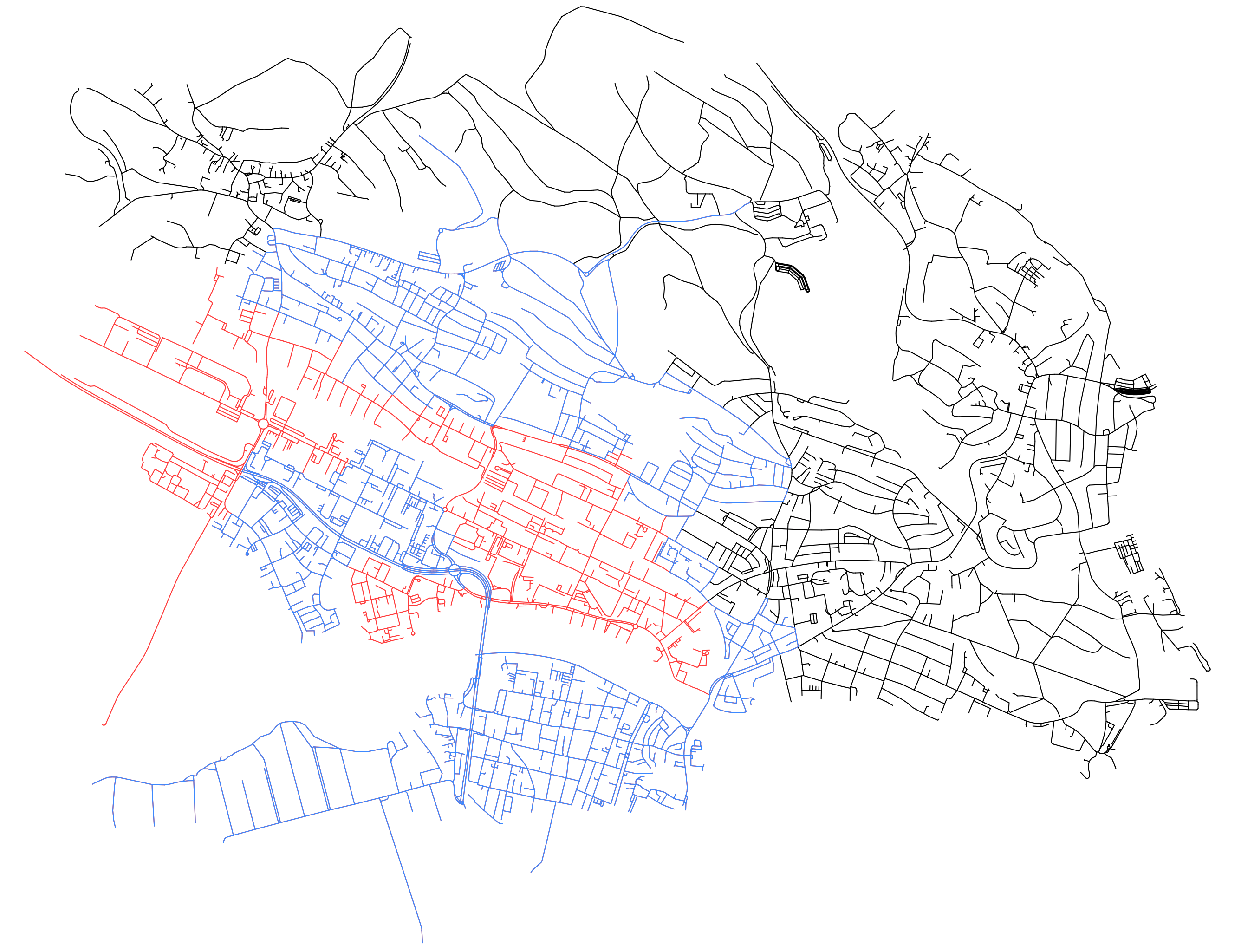
This completes the proof of Theorem 1. By recursively applying the theorem to a given connected input graph until we end up with single edges, we can derive in time an edge partition tree of depth , in which each node encodes a connected subgraph of . Figure 3 illustrates this partitioning. Next, we discuss how to augment the resulting edge partitioning tree structure to cater for circle-segment queries.
3.2 Circle-Graph Intersection Oracles
Given a connected graph , our goal is to construct an efficient decision oracle that returns true if a given query circle has a type(i)- or a type(ii)- intersection with some edge in and false otherwise.
For our oracle, we utilize the well known geometric transformation in which points are mapped to points by a projection function , and a circle with center and radius is mapped to the plane in by a function such that is inside iff lies below and outside iff lies above . These transformations are also applied in [16]. Let know denote the set of segment endpoints in the graph after applying the transformation via . Further let denote the convex hull of the resulting three-dimensional point set. We now show how these structures can be utilized to detect intersections of type-(i).
Lemma 5.
Iff for a given connected graph and a circle the plane intersects there exists at least one edge which has a type-(i) intersection with .
Proof.
If intersects , it follows that there is at least one point above as well as at least one point below . By means of the applied geometric transformation, we know that lies outside of while lies inside of . As is connected, there needs to exist a path from to in , that is a path that starts outside the circle and ends in it. Accordingly, the path needs to contain at least one edge that crosses the circle boundary. It follows that and have a type-(i) intersection. Vice versa, if an edge that intersects exists, its endpoints are projected to different halfspaces with respect to and therefore it follows that intersects . Accordingly, the oracle returns if intersects . Otherwise, if the convex hull is either completely below or above , we know that a type-(i) intersection can not occur but we still have to check for type-(ii) intersections. By definition of a type-(ii) intersection, the endpoints of the respective edge both need to be outside of the query circle. Thus, the oracle can safely return false if is completely below as in this case all edge endpoints are inside the circle. So from now on, we only consider the case that lies completely above .
Lemma 6.
Given a set of edge segments with all segment endpoints being outside of a circle , then there exists a type-(ii) intersection between a segment in and iff there exists a segment such that .
Proof.
Let be the segment closest to the circle center . If , we know that no segment in penetrates the circle and thus there is no type-(ii) intersection. Otherwise, if we know that has a type-(ii) intersection with as both segment endpoints are outside the circle but the point on the segment closest to the circle center is inside the circle or on its boundary, which matches the definition of a type-(ii) intersection. Based on Lemma 5 and Lemma 6, we now have a full description of our decision oracle: Return true if , or, if lies completely above and there is a segment within distance from the circle center. Return false otherwise. The following theorem analyzes the construction and query time of this oracle.
Theorem 7.
Given a connected geometric graph with edges and a query circle , an oracle which decides in time whether any graph edge intersects can be constructed in time and space, where is the number of edge crossings in .
Proof.
For the first part of the oracle, we construct a Dobkin-Kirkpatrick hierarchy on the edge segment endpoints projected into . The Dobkin-Kirkpatrick hierarchy data structure can be computed in time and space on a set of points and allows to answer extreme point queries in time [13, 14]. For the plane , we issue two extreme point queries, one using the normal of the plane as optimization direction and one using the negated normal. The result will always be corner points of . If both points are below/above , then is fully below/above . If one point is below and the other one above, we know that .
For the second part of the oracle, we need a data structure that reports the closest segment to a given query point (the circle center). We use a Segment Voronoi Diagram (SVD) for this purpose. It can be constructed in time and space, where is the number of edge crossings in [17]. Nearest-segment queries can be answered in time . Thus, the second part of the oracle dominates the construction and query time.
3.3 Query Answering
We are now ready to describe and analyze the full circle-segment data structure and the respective query answering algorithm.
Combining the insights from Theorem 1 and Theorem 7, we first construct an edge partition tree data structure, in which each node represents a connected subgraph of , and then equip each such node with a decision oracle. To report all segment intersection with a query circle , we first apply the transformation to the three-dimensional plane . Then, we use the following recursive algorithm for query answering, with the initial call being to root node of our data structure: For the current data structure node, which represents some connected edge subset , we ask the associated oracle whether there is any segment in that intersects . If the answer is false, we stop. Otherwise, if the answer is true, we recursively call the algorithm on both children of the current node. We also stop if we reach a leaf node, which represents a single segment, and include this segment in the output set if it indeed intersects . Figure 4 illustrates the query answering process on a small example graph.
Theorem 8.
We can build a circle-segment data structure on the edges of a connected geometric graph with edge crossings in time and space, which reports the segments that intersect a given query circle in time.
Proof.
The construction time and the size of the data structure is dominated by the oracle computation for each subgraph represented in the edge partition tree. As the tree has logarithmic depth by virtue of Theorem 1 and the computation time is in per level by virtue of Theorem 7, we get a total construction time in .
A query traverses the tree data structure in a DFS-like manner, aborting the search at nodes for which the oracle has concluded that there are no intersections to be detected in the respective subtree. Clearly, if the oracle answers true for any internal node of the tree, then at least for one if its children the answer needs to be true as well, as the segment inducing an intersection with the query circle has to be contained in either of the respective subgraphs. Therefore, the oracle calls in which the answer is false can always be charged to their respective siblings for which the answer is true (with the exception of the answer being false immediately on the root node). The number of times the oracle returns true is upper bounded by the number of nodes on a root-to-leaf path to segments that do intersect the query circle. As there are such segments and a root-to-leaf path has a length in , there are at most such successful oracle calls. According to Theorem 7, each oracle call takes time, and therefore we end up with a total query time in .
We remark that our data structure can also easily be used to answer disk queries with the same performance bounds. The only difference is that during query answering, whenever we encounter a node which represents a subgraph for which lies completely below , we add all edges in to the output set and still abort the search at this node.
4 Proof-Of-Concept Study
To demonstrate the usefulness of our circle-segment intersection data structure for practical application, we implemented the construction algorithm and the query answering routine in C++ and tested them on real-world road networks extracted from OSM. Experiments were conducted on an AMD Ryzen Threadripper 3970X with 32 cores.
4.1 Baseline
As baseline, we use the the AABB tree implementation provided by CGAL. It is a hierarchical data structure, in which each leaf node stores a geometric object and each internal node stores the bounding rectangle of all the objects in the respective subtree. It is constructed by dividing the input set of geometric objects roughly in half, computing the respective bounding rectangles, and then continuing recursively on both subsets until the leaf nodes are reached, which store the objects themselves. In our case, the leaves store the segments of the input graph . In a query, given a geometric object, we check whether its bounding rectangle intersects the bounding rectangle associated with the root node of the AABB tree. If this is the case, both children are checked as well. If not, the search is aborted at the respective node. If a leaf node is reached and the final check confirms an intersection, the geometric object stored in said leaf node is added to the output. While often fast in practice, the theoretical running time can be huge in the case that the bounding rectangle of the query object intersects many bounding rectangles associated with the tree nodes, but there are no actual intersections between the query object and the elements stored in the tree leaves. This happens particularly often if the query object is not an area (as a disk) but rather an area boundary (as a circle). Here, any segment fully contained in the circle will create a bounding rectangle that intersects the one of the circle, although the segment itself does not intersect the circle. To improve the performance of our baseline, we therefore do not query the segment AABB tree with the bounding rectangle of the circle, but instead cover the circle with eight rectangles of much smaller total area, see Figure 5. We refer to this method as the refined AABB query.
4.2 Comparative Evaluation
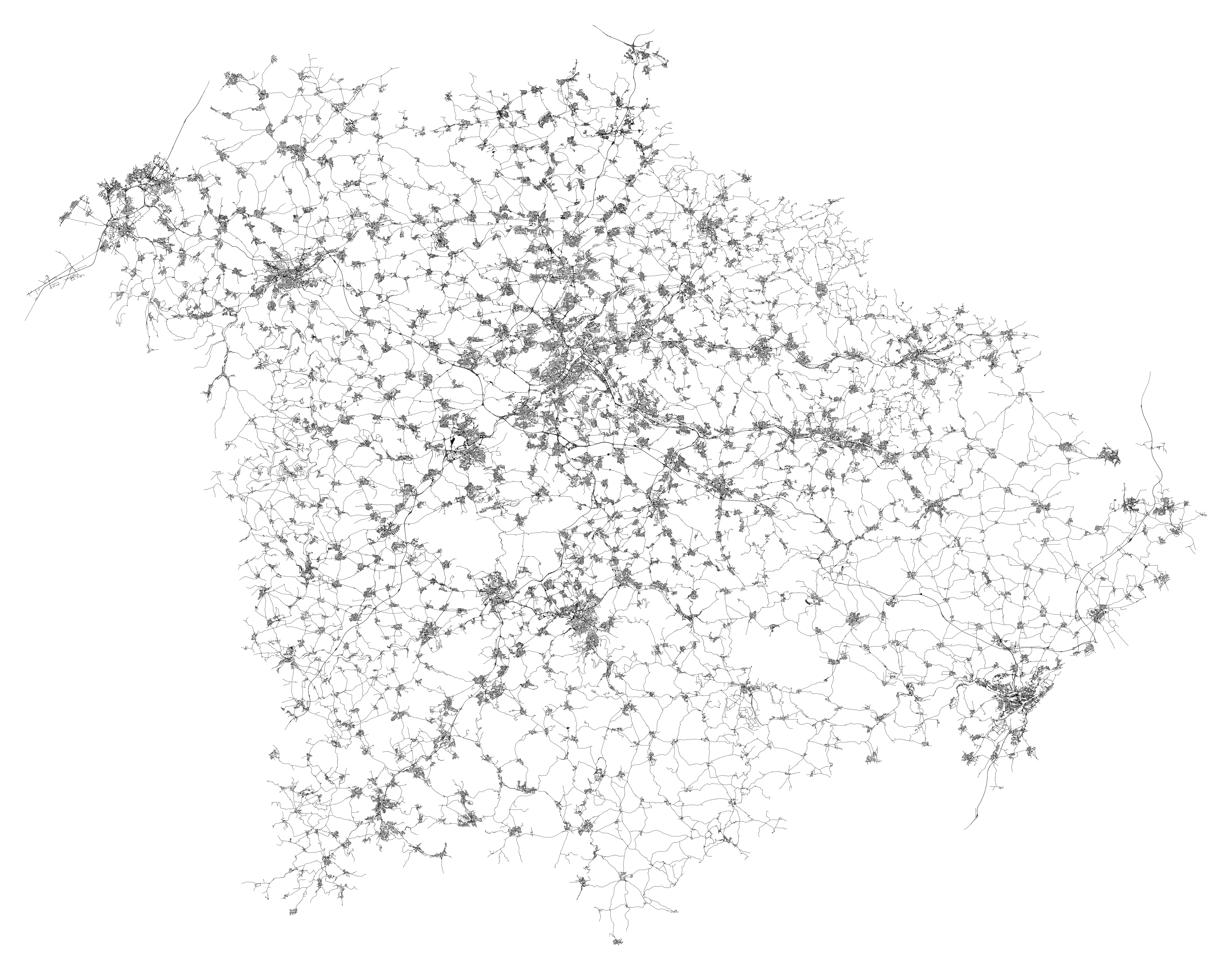
As benchmarks, we used two large real-world road networks, namely a part of Germany (Figure 6) with roughly 1.1 million edges and the road network of Taiwan (Figure 8) with about 5 million edges. The Germany graph has edge crossings and the Taiwan graph .
Constructing our circle-segment intersection data structure took less than 12 minutes on the Germany graph. The construction time is dominated by the segment Voronoi diagram computations for all subgraphs contained in the edge partition tree. In Figure 7, we compare the query times of our data structure to those of the refined AABB queries. We observe that except for very small query circle radii, our data structure is clearly superior. Even for large output sizes, the query times stay below 30 milliseconds and are at the peak about a factor of 8 faster than the respective refined AABB queries and two orders of magnitude faster than the naive AABB queries. Thus, we only consider the refined AABB queries in the upcoming experiments. We think that the mild increase of the query time with the output size besides the shown theoretical running time of can be explained by many paths from the root to a leaf that contain an intersecting segment share long common prefixes (while the theoretical worst-case analysis assumes them to be disjoint). Moreover, most of the occurring intersections are of type-(i). Our circle-graph oracle confirms such an intersection in time and then does not need to call the more expensive oracle for a type-(ii) intersection. Thus, in practice we have fewer and more efficient oracle calls than assumed in the theoretical analysis.
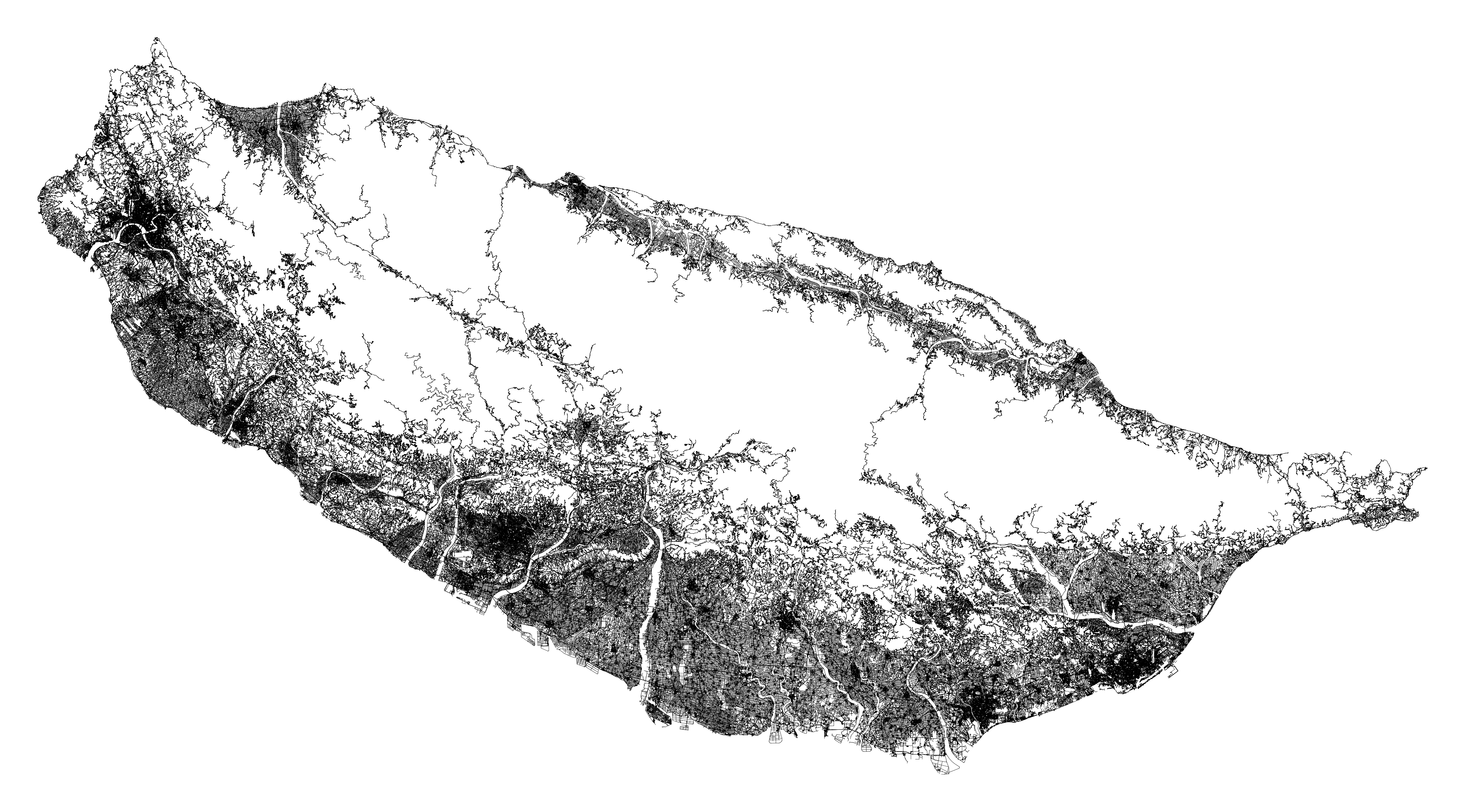
To deal with even larger graphs within a reasonable construction time, we observe that we can cut the top of our edge partition tree as well as the bottom levels. If we cut top levels, we then have to deal on query time with multiple root nodes, but we avoid the most expensive oracle construction steps on the large edge partitions close to the root. We remark that multiple root nodes can also be used in case the input graph is not connected but consists of (few) connected components. Cutting the bottom levels implies that we stop the recursive edge partitioning approach not only if we are down to single segments but already when the partition size drops below a certain threshold . For the resulting leaf nodes, we do not construct the circle-graph intersection oracles but instead perform a simple intersection check for each contained segment with the query circle. As this limits the number of tree nodes, it helps to safe space. Furthermore, it is expected that the rather complex oracles we construct are only effective if the respective segment size is sufficiently large. We applied top and bottom cutting to the road network of Taiwan. This reduces the construction time significantly, from more than an hour to roughly 9 minutes. In Figure 9, we measure the impact of these data structure engineering techniques on the query time. Again, we observe that the refined AABB query times increase significantly with the query radius and the output size, reaching up to about half a second. Our query times, however, are again in the 20-40 millisecond range, although the search now starts from 76 root nodes (for most of which the oracle immediately returned a negative answer).
While it would of course also be interesting to conduct experiments on other types of graphs (for example, triangle meshes), our proof-of-concept study clearly shows the potential of our newly proposed data structure to accelerate the circle-segment queries on connected geometric graphs even for large edge sets.
5 Conclusions and Future Work
In this paper, we introduced a novel data structure for circle-segment intersection queries on connected geometric graphs. We proved a near-linear construction time in the size of the segment set and the number of crossings among the input segments, as well as output-sensitive query times. The data structure was also confirmed to perform well in practice. Nevertheless, there are many ways in which our data structure might be further improved:
-
At the moment, we compute the circle-graph intersection oracle independently for each node in our edge partition tree. However, it might be much faster to compute the Dobkin-Kirkpatrick hierarchy and the segment Voronoi diagram bottom-up, using randomized incremental algorithms or clever merging strategies to derive the proper data structures for the level above from the already computed solutions from below. This might allow to decrease the construction time, both in theory and practice.
-
Fractional cascading is often used to improve query times if the query involves repeated (binary) searches over similar or nested structures [10]. Recently, it was shown that for an input graph with bounded degree and a set of hyperplanes in 3D associated with each node in , one can decide for a query point and a connected subgraph of wether the point is below or above the lower envelope of the hyperplanes associated with the nodes in much faster using fractional cascading [2]. Adapting this methodology to our use case, where we perform searches over nested convex hulls when we traverse the tree, could help to further improve our query times.
It would also be interesting to obtain lower bounds for data size and query time trade-offs in the connected graph setting to see how much improvement is still possible in theory. Moreover, integrating additional engineering ideas could also increase the scalability of the data structure and therefore make it useful for an even larger range of practical applications.
References
- [1] Ahmed Abdelkader and David M Mount. Approximate nearest-neighbor search for line segments. In 37th International Symposium on Computational Geometry, 2021.
- [2] Peyman Afshani, Yakov Nekrich, and Frank Staals. Convexity helps iterated search in 3d. In 41st International Symposium on Computational Geometry (SoCG 2025). Schloss Dagstuhl – Leibniz-Zentrum für Informatik, 2025. doi:10.4230/LIPIcs.SoCG.2025.3.
- [3] Pankaj K. Agarwal and M van Kreveld. Connected component and simple polygon intersection searching. Algorithmica, 15(6):626–660, 1996. doi:10.1007/BF01940884.
- [4] Pankaj K Agarwal, Marc van Kreveld, and Mark Overmars. Intersection queries for curved objects. In Proceedings of the seventh annual symposium on Computational geometry, pages 41–50, 1991.
- [5] Alok Aggarwal, Mark Hansen, and Thomas Leighton. Solving query-retrieval problems by compacting voronoi diagrams. In Proceedings of the twenty-second annual ACM symposium on Theory of computing, pages 331–340, 1990.
- [6] Julien Basch, Leonidas J Guibas, and GD Ramkumar. Reporting red-blue intersections between two sets of connected line segments. In Algorithms – ESA’96: Fourth Annual European Symposium Barcelona, Spain, September 25–27, 1996 Proceedings 4, pages 302–319. Springer, 1996.
- [7] Michael A Bender, Martin Farach-Colton, Giridhar Pemmasani, Steven Skiena, and Pavel Sumazin. Lowest common ancestors in trees and directed acyclic graphs. Journal of Algorithms, 57(2):75–94, 2005. doi:10.1016/J.JALGOR.2005.08.001.
- [8] Yannick Bosch and Sabine Storandt. Continuous map matching to paths under travel time constraints. In 23rd International Symposium on Experimental Algorithms, SEA 2025, July 22-24, 2025, Venice, Italy, volume 338 of LIPIcs, pages 7:1–7:17. Schloss Dagstuhl – Leibniz-Zentrum für Informatik, 2025. doi:10.4230/LIPICS.SEA.2025.7.
- [9] Florian Bourse, Marc Lelarge, and Milan Vojnovic. Balanced graph edge partition. In Proceedings of the 20th ACM SIGKDD international conference on Knowledge discovery and data mining, pages 1456–1465, 2014. doi:10.1145/2623330.2623660.
- [10] Bernard Chazelle and Leonidas J Guibas. Fractional cascading: I. a data structuring technique. Algorithmica, 1(1):133–162, 1986. doi:10.1007/BF01840440.
- [11] Daniel Chen, Anne Driemel, Leonidas J Guibas, Andy Nguyen, and Carola Wenk. Approximate map matching with respect to the fréchet distance. In 2011 Proceedings of the Thirteenth Workshop on Algorithm Engineering and Experiments (ALENEX), pages 75–83. SIAM, 2011. doi:10.1137/1.9781611972917.8.
- [12] Mark De Berg. Computational geometry: algorithms and applications. Springer Science & Business Media, 2000.
- [13] David P Dobkin and David G Kirkpatrick. Fast detection of polyhedral intersection. Theoretical computer science, 27(3):241–253, 1983. doi:10.1016/0304-3975(82)90120-7.
- [14] David P Dobkin and David G Kirkpatrick. Determining the separation of preprocessed polyhedra—a unified approach. In International Colloquium on Automata, Languages, and Programming, pages 400–413. Springer, 1990. doi:10.1007/BFB0032047.
- [15] David Eppstein and Michael T Goodrich. Studying (non-planar) road networks through an algorithmic lens. In Proceedings of the 16th ACM SIGSPATIAL international conference on Advances in geographic information systems, pages 1–10, 2008.
- [16] Prosenjit Gupta, Ravi Janardan, and Michiel Smid. On intersection searching problems involving curved objects. In Algorithm Theory – SWAT’94: 4th Scandinavian Workshop on Algorithm Theory Aarhus, Denmark, July 6–8, 1994 Proceedings 4, pages 183–194. Springer, 1994. doi:10.1007/3-540-58218-5_17.
- [17] Menelaos I Karavelas. A robust and efficient implementation for the segment voronoi diagram. In International symposium on Voronoi diagrams in science and engineering, volume 2004, pages 51–62, 2004.
- [18] Hung Le and Cuong Than. Greedy spanners in euclidean spaces admit sublinear separators. ACM Transactions on Algorithms, 20(3):1–30, 2024.
- [19] Jiří Matoušek. Efficient partition trees. In Proceedings of the seventh annual symposium on Computational geometry, pages 1–9, 1991.
- [20] Harvey J Miller. Gis and geometric representation in facility location problems. International Journal of Geographical Information Systems, 10(7):791–816, 1996. doi:10.1080/02693799608902110.
- [21] A Frank Van der Stappen and Mark H Overmars. Motion planning amidst fat obstacles. In Proceedings of the tenth annual symposium on Computational geometry, pages 31–40, 1994.
- [22] Chenzi Zhang, Fan Wei, Qin Liu, Zhihao Gavin Tang, and Zhenguo Li. Graph edge partitioning via neighborhood heuristic. In Proceedings of the 23rd ACM SIGKDD International Conference on Knowledge Discovery and Data Mining, pages 605–614, 2017. doi:10.1145/3097983.3098033.