Matchgate Signatures Under Variable Permutations

Meng, Boning; Pan, Yicheng

doi:10.4230/LIPIcs.ISAAC.2025.50

Matchgate Signatures Under Variable Permutations

Boning Meng¹¹1First author.

Key Laboratory of System Software (Chinese Academy of Sciences) and State Key Laboratory of Computer Science, Institute of Software, Chinese Academy of Sciences, Beijing, China
University of Chinese Academy of Sciences, Beijing, China Yicheng Pan³³3Corresponding author.

State Key Laboratory of Complex & Critical Software Environment, Beihang University, Beijing, China

Abstract

In this work, we introduce the concept of permutable matchgate signatures and leverage it to establish dichotomy theorems for #CSP and # $R_{D}$ -CSP ( $D\geq 3$ ) on planar graphs without the variable ordering restriction. We also present a complete characterization of permutable matchgate signatures and their relationship to symmetric signatures. Besides, we give a sufficient and necessary condition for determining whether a matchgate signature retains its property under a certain variable permutation, which can be checked in polynomial time. In addition, we prove a dichotomy for Pl- $\#R_{D}$ -CSP ( $D\geq 3$ ), where the variable ordering restriction exists.

Keywords and phrases:

Computational Complexity, Matchgate Signature, Counting CSP

Funding:

Boning Meng: supported by National Key R&D Program of China (2023YFA1009500), NSFC 62532014 and NSFC 62272448.

Yicheng Pan: supported by State Key Laboratory of Complex & Critical Software Environment (SKLCCSE-2024ZX-20) and NSFC 61932002.

Copyright and License:

2012 ACM Subject Classification:

Theory of computation

\rightarrow

Problems, reductions and completeness

Related Version:

Full Version: https://arxiv.org/abs/2503.21194

Acknowledgements:

We want to thank Mingji Xia for introducing this problem to us.

DOI:

10.4230/LIPIcs.ISAAC.2025.50

Event:

36th International Symposium on Algorithms and Computation (ISAAC 2025)

Editors:

Ho-Lin Chen, Wing-Kai Hon, and Meng-Tsung Tsai

Series and Publisher:

Leibniz International Proceedings in Informatics, Schloss Dagstuhl – Leibniz-Zentrum für Informatik

1 Introduction

Counting perfect matchings in a graph (denoted by #PM) is of great significance in counting complexity. The study of #PM was motivated by the dimer problem in statistical physics [13, 14, 15, 19], and two fundamental results emerged from this study. The first breakthrough occurred in 1961, when a polynomial time algorithm for #PM on planar graphs was developed by Kasteleyn, Temperley and Fisher [14, 19], now known as the FKT algorithm. The second significant advancement occurred in 1979, when Valiant defined the complexity class #P and proved that #PM on general graphs is #P-hard [21]. #PM was the first natural counting problem discovered to be #P-hard on general graphs and polynomial-time computable on planar graphs.

Matchgates were later introduced to generalize the FKT algorithm. Multiple studies have been undertaken to systematically define and characterize matchgates [22, 23, 24, 2, 4, 18, 7, 16]. In particular, the matchgate is proved to be highly related to the complexity classification for counting constraint satisfaction problems (denoted by #CSP) on plane graphs over Boolean domain and complex range [12, 5].

In this article, we always restrict ourselves to Boolean domain and complex range. We further develop the theory of matchgates and establish new complexity classifications for a variant of #CSP. Our primary contribution is the introduction and detailed characterization of permutable matchgate signatures – a novel concept that enables complexity analyses for #CSP variants, such as #CSP on planar graphs without the variable ordering restriction.

Section 1.1 and Section 1.2 introduce the existing results regarding matchgates and #CSP. Section 1.3 explains our motivation and presents our results.

1.1 #PM and matchgate signatures

For a graph $G=(V,E)$ , a matching is an edge set $M\subseteq E$ such that no pair of edges in $M$ shares a common endpoint. Besides, if the vertices that $M$ contains are exactly $V(M)=V$ , then $M$ is a perfect matching of $G$ .

Definition 1.

An instance of #PM is a graph $G=(V,E)$ with weighted edges $w:E\to\mathbb{C}$ . The weight of a matching $M$ is $w(M)=\prod_{e\in M}w(e)$ . The output of the instance is the sum of the weights of all perfect matchings in $G$ :

\text{\#PM}(G)=\sum_{M:M\text{ is a perfect matching of }G}w(M).

When $w(e)=1$ for each $e\in E$ , the output of the instance is exactly the number of perfect matchings in the graph.

Matchgate and their associated matchgate signatures are defined in the context of #PM. A signature (also referred to as a constraint function in some works) is defined as a function $f:\{0,1\}^{k}\to\mathbb{C}$ that maps a string of length $k$ to a complex number. For $G=(V,E)$ and $X\subseteq V$ , we use $G-X$ to denote the graph obtained by deleting vertices in $X$ from $G$ .

Definition 2.

A matchgate is a plane graph $G=(V,E)$ with weighted edges $w:E\to\mathbb{C}$ , and together with some external nodes $U\subseteq V$ on its outer face labelled by $\{1,2,...,|U|\}$ in a clockwise order. The signature $f$ of a matchgate $G$ is a Boolean signature of arity $|U|$ and for each $\alpha\in\{0,1\}^{|U|}$ ,

f(\alpha)=\#PM(G-X),

where $X\subseteq U$ and a vertex in $U$ with label $i$ belongs to $X$ if and only if the $i$ th bit of $\alpha$ is 1.

A signature $f$ is a matchgate signature if it is the signature of some matchgate. $\mathscr{M}$ denotes all the matchgate signatures.

Matchgates provide a generalization of the FKT algorithm in the following way. Suppose $G$ is a plane graph with each vertex $v$ representing some matchgate signature, forming a signature grid. By replacing each vertex $v$ with its corresponding matchgate $H$ , the resulting graph $G^{\prime}$ remains a plane graph and consequently $\#PM(G^{\prime})$ can be solved in polynomial time by the FKT algorithm. Consequently, the value of the signature grid $G$ , which is exactly $\#PM(G^{\prime})$ , can be computed in polynomial time.

In particular, a so-called matchgate identity (MGI) has been verified to be the necessary and sufficient condition for a signature to be a matchgate signature [2, 4, 7], which provides an algebraic way to characterize matchgate signatures. This identity also enables an universal way to construct a corresponding matchgate for a matchgate signature.

Theorem 3 (MGI).

Suppose $f$ is a signature of arity $k$ . Then $f$ is a matchgate signature if and only if the following identity, denoted by MGI, is satisfied:

For each $\beta,\gamma\in\{0,1\}^{k}$ , let $P=\{1\leq j\leq k|\beta_{j}\neq\gamma_{j}\}$ , $l=|P|$ . Let $p_{j}\in P$ be the $j$ th smallest number in $P$ and let $e_{p_{j}}\in\{0,1\}^{k}$ denotes a string with a 1 in the $p_{j}$ th index, and 0 elsewhere. Then

\sum_{j=1}^{n}(-1)^{j}f(\beta\oplus e_{p_{j}})f(\gamma\oplus e_{p_{j}})=0.

Lemma 4 ([7]).

A matchgate signature of arity $k$ can be realized by a matchgate with at most $O(k^{4})$ vertices, which can be constructed in $O(k^{4})$ time.

1.2 #CSP

A counting constraint satisfaction problem is specified by a signature set $\mathcal{F}$ . $\#\text{CSP}(\mathcal{F})$ asks for the value of an instance, which is the sum of the values over all configurations. Here, $\mathcal{F}$ is a fixed and finite set of signatures. An instance of $\text{\#CSP}(\mathcal{F})$ is specified as follows:

Definition 5 (#CSP [10]).

An instance $I$ of $\#\text{CSP}(\mathcal{F})$ has $n$ variables and $m$ signatures from $\mathcal{F}$ depending on these variables. The value of the instance then can be written as

Z(I)=\sum_{(x_{1},...,x_{n})\in\{0,1\}^{n}}\prod_{1\leq i\leq m}f_{i}(x_{i_{1}% },...,x_{i_{k}}),

where $f_{1},\dots,f_{m}$ are signatures in $I$ and $f_{i}$ depends on $x_{i_{1}},...,x_{i_{k}}$ for each $1\leq i\leq m$ .

The underlying graph of a $\text{\#CSP}(\mathcal{F})$ instance $I$ is its incidence graph. It is a bipartite graph $G=(U,V,E)$ , where for every constraint $f$ there is a $u_{f}\in U$ , for every variable $x$ there is a $v_{x}\in V$ , and $(u_{f},v_{x})\in E$ if and only if $f$ depends on $x$ . See Figure 1 for an example. Sometimes we also denote the value $Z(I)$ as $Z(G)$ for convenience.

There are several important variants of #CSP. A signature $f$ is said to be symmetric if the output of $f$ depends only on the Hamming weight of the input. If each signature in $\mathcal{F}$ is restricted to be symmetric, this kind of problem is denoted by symmetric #CSP, or sym-#CSP for short. If the maximum degree of the vertices in $V$ is at most a constant $D\geq 3$ , this kind of problem is denoted by $\#R_{D}$ -CSP [9]. If each vertex in $V$ is of degree 2, this kind of problem is denoted by Holant [8] (See Definition 15 for details). If we restrict $G$ to be a plane graph, in which the variables that $f_{u}$ depends on are ordered clockwise for each $u\in U$ (denoted by the variable ordering restriction), then we denote this problem as Pl-#CSP. Pl- $\#R_{D}$ -CSP is defined similarly.

To study the complexity of these problems, a number of dichotomy theorems have been established, which classify that for each signature set, the specified problem is either polynomial-time computable or #P-hard. $\mathscr{A}$ and $\mathscr{P}$ are two fundamental tractable signature sets, whose definition can be found in [9]. $\widehat{\mathscr{M}}$ denote the matchgate signatures under a specific holographic transformation explained later in Section 2.2.2.

Theorem 6 ([9]).

If $\mathcal{F}\subseteq\mathscr{A}$ or $\mathcal{F}\subseteq\mathscr{P}$ , then $\text{\#CSP}(\mathcal{F})$ is polynomial-time computable; otherwise it is #P-hard.

Theorem 7 ([9]).

Suppose $D\geq 3$ is an integer. If $\mathcal{F}\subseteq\mathscr{A}$ or $\mathcal{F}\subseteq\mathscr{P}$ , then $\#R_{D}\text{-CSP}(\mathcal{F})$ is polynomial-time computable; otherwise it is #P-hard.

Theorem 8 ([5]).

If $\mathcal{F}\subseteq\mathscr{A}$ or $\mathcal{F}\subseteq\mathscr{P}$ or $\mathcal{F}\subseteq\widehat{\mathscr{M}}$ , then $\text{Pl-\#CSP}(\mathcal{F})$ is polynomial-time computable; otherwise it is #P-hard.

1.3 Motivation and results

The study of counting complexity has been extended to a number of different graph classes. In particular, the complexity of #PM on minor-excluded graphs has been fully classified by [11, 20]. These results generalize the FKT algorithm and the #P-hardness of #PM on general graphs. It is natural to consider adapting other counting algorithms and hardness results related to #PM, such as the dichotomy for #CSP, to the minor-excluded setting. However, existing results on Pl-#CSP rely on the variable ordering restriction, a restriction for the signatures rather than the graph class. This limitation obstructs the direct extension of Pl-#CSP to broader graph families.

To overcome this limitation, we focus on #CSP on planar graphs without the variable ordering restriction. We use $\mathcal{PL}$ to denote the class of planar graphs and #CSP $(\mathcal{F})\langle\mathcal{PL}\rangle$ to denote #CSP specified by the signature set $\mathcal{F}$ over the graph class $\mathcal{PL}$ . #CSP $(\mathcal{F})\langle\mathcal{PL}\rangle$ is exactly #CSP on planar graphs without the variable ordering restriction.

Before investigating #CSP $\langle\mathcal{PL}\rangle$ , we also observe that the complexity classification for Pl- $\#R_{D}$ -CSP remains open in the literature. To address this gap, we establish the following result:

Theorem 9.

Suppose $D\geq 3$ is an integer. If $\mathcal{F}\subseteq\mathscr{A}$ or $\mathcal{F}\subseteq\mathscr{P}$ or $\mathcal{F}\subseteq\widehat{\mathscr{M}}$ , Pl- $\#R_{D}$ -CSP $(\mathcal{F})$ is polynomial-time computable; otherwise it is #P-hard.

The full proof of Theorem 9 is similar to that of Theorem 7 originally presented in in [9, Section 6], and can be found in the full version. Here, we only remark the major differences between the two proofs.

$\blacksquare$

All the gadgets in our proof are constructed in the setting of Pl- $\#R_{D}$ -CSP instead of $\#R_{D}$ -CSP;
$\blacksquare$

Unlike [9, Lemma 6.5], we realize $[0,0,1]=[0,1]^{\otimes 2}$ instead of $[0,1]^{\otimes m}$ ;
$\blacksquare$

Unlike [9, Lemma 6.2], instead of realizing a single non-degenerate binary signature $h$ , we realize $h^{\otimes 2}$ and use them to form a non-degenerate binary signature $g=h^{T}h$ .

Returning to the framework of #CSP $\langle\mathcal{PL}\rangle$ , we demonstrate that the concept of permutable matchgate signatures plays a pivotal role in establishing its dichotomy theorem in a straightforward way.

Definition 10 (Permutable matchgate signature).

Suppose $f$ is a signature of arity $n$ . For a permutation $\pi\in S_{n}$ , we use $f_{\pi}$ to denote the signature

f_{\pi}(x_{1},\dots,x_{n})=f(\pi(x_{1}),\dots,\pi(x_{n}))

If for each $\pi\in S_{n}$ , $f_{\pi}$ is a matchgate signature, we say $f$ is a permutable matchgate signature.

We use $\mathscr{M}_{P}$ to denote the set of all the permutable matchgate signatures.

Theorem 11.

Let $\mathcal{F}$ be a finite signature set and $D\geq 3$ be an integer.

If $\mathcal{F}\subseteq\mathscr{A}$ or $\mathcal{F}\subseteq\mathscr{P}$ or $\mathcal{F}\subseteq\widehat{\mathscr{M}_{P}}$ , $\#\text{CSP}(\mathcal{F})\langle\mathcal{PL}\rangle$ is polynomial-time computable; otherwise it is #P-hard.

If $\mathcal{F}\subseteq\mathscr{A}$ or $\mathcal{F}\subseteq\mathscr{P}$ or $\mathcal{F}\subseteq\widehat{\mathscr{M}_{P}}$ , $\#R_{D}\text{-CSP}(\mathcal{F})\langle\mathcal{PL}\rangle$ is polynomial-time computable; otherwise it is #P-hard.

Proof.

Let $\mathcal{F^{\prime}}=\{f_{\pi}|f\in\mathcal{F},\text{arity}(f)=n,\pi\in S_{n}\}$ . Then we have $\text{\#CSP}(\mathcal{F})\langle\mathcal{PL}\rangle\equiv_{T}\text{Pl-\#CSP}(% \mathcal{F^{\prime}})$ . By Definitions of $\mathscr{A}$ and $\mathscr{P}$ , $\mathcal{F^{\prime}}\subseteq\mathscr{A}$ or $\mathscr{P}$ if and only if $\mathcal{F}\subseteq\mathscr{A}$ or $\mathscr{P}$ respectively. Furthermore, $\mathcal{F^{\prime}}\subseteq\widehat{\mathscr{M}}$ if and only if $\mathcal{F}\subseteq\widehat{\mathscr{M}_{P}}$ by Definition 10. Consequently, we are done by replacing the tractable criteria for $\mathcal{F^{\prime}}$ in Theorem 8 with those for $\mathcal{F}$ . The same argument holds for $\#R_{D}\text{-CSP}\langle\mathcal{PL}\rangle$ as well. $\hfill\blacktriangleleft$

The main contribution of this article is a detailed characterization of permutable matchgate signatures, showing the connection between them and symmetric matchgate signatures. This characterization has been proved to be useful in the algorithm design and the hardness proof in the subsequent work [17]. A signature $f$ is said to be realized by $\mathcal{F}$ if it can be simulated using signatures in $\mathcal{F}$ under polynomial-time Turing reduction.

Theorem 12 (Informal version of Theorem 25).

Each permutable matchgate signature of arity $n$ can be realized by a symmetric matchgate signature of arity $n$ and $O(n)$ binary matchgate signatures.

Theorem 13 (Informal version of Theorem 26).

For each permutable matchgate signature $f$ , if # $R_{3}$ -CSP $(\{f\})$ is #P-hard, then a symmetric matchgate signature $g$ , satisfying # $R_{3}$ -CSP $(\{g\})$ is #P-hard, can be realized by $f$ and 3 specific matchgate signatures $[1,0],[1,0,1],[1,0,1,0]$ .

It is noteworthy that there are actually three types of permutable matchgate signatures (Pinning, Parity, Matching) possess different properties, but they are all related to the corresponding symmetric matchgate signatures by our proof.

In addition, we also present a sufficient and necessary condition for determining whether a matchgate signature retains its property under a specific variable permutation. This condition is a simplified version of the MGI property, since it only requires considering $O(n^{4})$ equations from MGI rather than all $O(2^{n})$ equations.

Theorem 14 (Informal version of Theorem 22).

Suppose $f$ is a matchgate signature satisfying $f(\vec{0})\neq 0$ and $\pi$ is a permutation. Then $f_{\pi}$ retains MGI if $O(n^{4})$ specific equations from MGI are still satisfied.

The proof of this theorem is inspired by an alternative proof of Theorem 3, given by Jerrum and recorded in [1, Section 4.3.1]. By dividing the summation in MGI into appropriate parts, we prove this result by a non-trivial induction.

2 Preliminaries

2.1 Counting problems

For a string $\alpha=\alpha_{1}\dots\alpha_{k}\in\{0,1\}^{k}$ , the Hamming weight of $\alpha$ is the number of $1$ s in $\alpha$ , denoted by $HW(\alpha)$ . We use $\overline{\alpha}$ to denote the string that differs from $\alpha$ at every bit, which means $\alpha_{i}+\overline{\alpha}_{i}=1$ for each $1\leq i\leq k$ .

For a signature $f:\{0,1\}^{k}\to\mathbb{C}$ , $k$ is denoted by the arity of $f$ . A symmetric signature $f$ of arity $k$ can be denoted by $[f_{0},f_{1},...,f_{k}]_{k}$ , or simply $[f_{0},f_{1},...,f_{k}]$ when $k$ is clear from the context, where for $0\leq i\leq k$ , $f_{i}$ is the value of $f$ when the Hamming weight of the input is $i$ . For $c\in\mathbb{C}$ , we also use the notation $c[f_{0},f_{1},...,f_{k}]$ to denote the signature $[cf_{0},cf_{1},...,cf_{k}]$ . We use $\leq_{T}$ and $\equiv_{T}$ to respectively denote polynomial-time Turing reduction and equivalence. We denote by $f^{x_{i}=c}$ the signature that pins the $i$ th variable to $c\in\{0,1\}$ :

f^{x_{i}=c}(x_{1},...,x_{i-1},x_{i+1},...,x_{k})=f(x_{1},...,x_{i-1},c,x_{i+1}% ,...,x_{k}).

2.1.1 Holant problems

A Holant problem $\text{Holant}(\mathcal{F})$ can be seen as a $\text{\#CSP}(\mathcal{F})$ problem with the restriction that all the variables must appear exactly twice.

Definition 15.

An instance of $\text{Holant}(\mathcal{F})$ has an underlying graph $G=(V,E)$ . Each vertex $v\in V$ is assigned a signature from $\mathcal{F}$ and each edge in $E$ represents a variable. Here, $\mathcal{F}$ is a fixed set of signatures and usually finite. The signature assigned to the vertex $v$ is denoted by $f_{v}$ . An assignment of $E$ is a mapping $\sigma:E\to\{0,1\}$ , which can also be expressed as an assignment string $\sigma\in\{0,1\}^{|E|}$ , and the value of the assignment is defined as

\omega(\sigma)=\prod_{v\in V}f_{v}(\sigma),

where $f_{v}(\sigma)=f_{v}(\sigma({e_{v_{1}}}),...,\sigma({e_{v_{k}}}))$ and $v$ is incident to $e_{v_{1}},...,e_{v_{k}}$ .

The output of the instance, or the value of $G$ , is the sum of the values of all possible assignments of $E$ , denoted by:

Z(G)=\sum_{\sigma\in\{0,1\}^{|E|}}\omega(\sigma).

Furthermore, we use $\text{Holant}(\mathcal{F}_{1}|\mathcal{F}_{2})$ represents $\text{Holant}(\mathcal{F}_{1}\cup\mathcal{F}_{2})$ with the restriction that the underlying graph $G=(U,V,E)$ is bipartite, and each vertex $u\in U$ is assigned a signature from $\mathcal{F}_{1}$ while each vertex $v\in V$ is assigned a signature from $\mathcal{F}_{2}$ . We denote by $\mathcal{EQ}$ the set of all equality functions. In other words, $\mathcal{EQ}=\{=_{k}|k\geq 1\}$ where $=_{k}$ is the signature $[1,0,...,0,1]_{k}$ . We also denote $\{=_{k}|1\leq k\leq D\}$ by $\mathcal{EQ}_{\leq D}$ for each integer $D\geq 1$ . By definition, we have the following lemma. Also see Figure 1 for an example.

Lemma 16.

Let $\mathcal{C}$ be an arbitrary graph class, $\mathcal{F}$ be an arbitrary signature set and $D\geq 1$ be an integer. Then,

\#\text{CSP}(\mathcal{F})\langle\mathcal{C}\rangle\equiv_{T}\text{Holant}(% \mathcal{F}|\mathcal{EQ})\langle\mathcal{C}\rangle,

\#R_{D}\text{-CSP}(\mathcal{F})\langle\mathcal{C}\rangle\equiv_{T}\text{Holant% }(\mathcal{F}|\mathcal{EQ}_{\leq D})\langle\mathcal{C}\rangle.

Refer to caption — Figure 1: The underlying graph of a $\text{\#CSP}(\mathcal{F})$ instance if $f,g,h\in\mathcal{F}$ and $x, y, z$ are 3 variables; or that of a $\text{Holant}(\mathcal{F}|\mathcal{EQ})$ instance if we treat $x, y, z$ as $=_{3},=_{2},=_{1}$ and the edges as the variables instead.

2.2 Reduction methods

2.2.1 Constructing gadgets

A gadget of $\text{Holant}(\mathcal{F})$ has an underlying graph $GG=(V,E,D)$ , where $E$ is the set of normal edges and $D$ is the set of edges with only one endpoint, called dangling edges ⁵⁵5In order to differentiate from the notation of a graph, we use two capital letters to represent a gadget.. Each vertex in $G G$ is still assigned a signature from $\mathcal{F}$ . A signature $f$ of arity $|D|$ is said to be realized by $GG=(V,E,D)$ , if for each assignment $\alpha:D\to\{0,1\}$ , $f(\alpha)=\sum_{\sigma\in\{0,1\}^{|E|}}\omega(\alpha\sigma)$ , where $\alpha\sigma$ is the assignment of edges in $D\cup E$ . In this case, we also say $f$ can be realized by $\mathcal{F}$ . By constructing gadgets with existing signatures, we are able to realize desired signatures.

Lemma 17.

If $f$ can be realized by $\mathcal{F}$ , then $\text{Holant}(\mathcal{F})\equiv_{T}\text{Holant}(\mathcal{F}\cup\{f\})$ .

Also, we present some derivative concepts related to the concept of a gadget. A left-side gadget of $\text{Holant}(\mathcal{F}_{1}|\mathcal{F}_{2})$ has a bipartite underlying graph $GG=(U,V,E,D)$ , where each vertex $u\in U$ is assigned a signature from $\mathcal{F}_{1}$ , each vertex $v\in V$ is assigned a signature from $\mathcal{F}_{2}$ , $E$ is the set of normal edges and $D$ is the set of dangling edges. Furthermore, the endpoint of each dangling edge must belong to $U$ . It is easy to verify that, if $f$ can be realized by $G G$ , then $\text{Holant}(\mathcal{F}_{1}|\mathcal{F}_{2})\equiv_{T}\text{Holant}(\mathcal% {F}_{1}\cup\{f\}|\mathcal{F}_{2})$ . The right-side gadget is defined similarly except that the endpoint of each dangling edge must belong to $V$ .

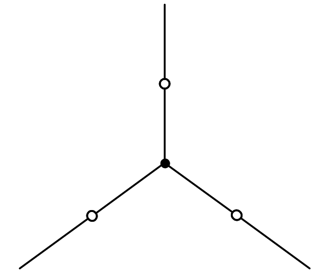
In the hardness proofs, we create generalized mating gadgets defined as follows, which is a generalization of the mating operation in [6]. In a generalized mating gadget, the variables of $F$ are divided into four parts: Sum-up variables, Fix-to-0 variables, Fix-to-1 variables and a single Dangling variable. We assign $F$ to each vertex of degree $n$ labelled by a solid circle in Figure 2 in the following way: for each $1\leq a\leq n$ , if the $a$ th variable is the Dangling variable, we let it correspond to the dangling edge. Otherwise we connect it to a vertex $v_{a}$ of degree 2 labelled by a hollow square. Furthermore, if the $a$ th variable is a Sum-up/Fix-to-0/Fix-to-1 variable, we assign a $[1,0,1]$ / $[1,0,0]$ / $[0,0,1]$ signature to $v_{a}$ , and the gadget become well defined. In such constructions, the $p+q$ variables corresponding to $[1,0]$ or $[0,1]$ are always Sum-up variables. We remark that using $[1,0]$ we may obtain the $[1,0,0]=[1,0]^{\otimes 2}$ signature, and we construct a gadget of $[0,0,1]$ when needed.

2.2.2 Holographic Transformation

Let $T$ be a binary signature, and we denote the two dangling edges corresponding to the input variables of it as a left edge and a right edge. Its value then can be written as a matrix $T=\begin{pmatrix}t_{00}&t_{01}\\ t_{10}&t_{11}\end{pmatrix}$ , where $t_{ij}$ is the value of $T$ when the value of left edge is $i$ and that of the right edge is $j$ .

This notation is conducive to the efficient calculation of the gadget’s value. Let us consider two binary signatures, $T$ and $P$ , with the right edge of $T$ connected to the left edge of $P$ . $T$ and $P$ now form a binary gadget. Subsequently, it can be demonstrated that the value of the resulting gadget is precisely $T P$ , which represents the matrix multiplication of $T$ and $P$ .

For a signature $f$ of arity $n$ and a binary signature $T$ , we use $Tf/fT$ to denote the signature “ $f$ transformed by $T$ ”, which is a signature of arity $n$ obtained by connecting the right/left edge of $T$ to every dangling edge of $f$ . For a set $\mathcal{F}$ of signatures, we also define $T\mathcal{F}=\{Tf|f\in\mathcal{F}\}$ . Similarly we define $\mathcal{F}T$ . The following theorem demonstrates the relationship between the initial and transformed problems:

Theorem 18 (Holographic Transformation[24, 3]).

$Holant(\mathcal{F}|\mathcal{G})\equiv_{T}Holant(\mathcal{F}T^{-1}|T\mathcal{G}).$

Let $H_{2}=\begin{pmatrix}1&1\\ 1&-1\end{pmatrix}$ . For a set of signatures $\mathcal{F}$ , we use $\widehat{\mathcal{F}}$ to denote $H_{2}\mathcal{F}$ . As $H_{2}^{-1}=\frac{1}{2}H_{2}$ , by Theorem 18 we have:

\text{Holant}(\mathcal{F}|\mathcal{G})\equiv_{T}\text{Holant}(\widehat{% \mathcal{F}}|\widehat{\mathcal{G}}).

We additionally present the following fact as a lemma for future reference.

Lemma 19.

For each $k\geq 1$ , $\widehat{=_{k}}=[1,0,1,0,1,0,\dots]_{k}$ . For example, $\widehat{=_{1}}=[1,0],\widehat{=_{2}}=[1,0,1],\widehat{=_{3}}=[1,0,1,0]$ . Consequently, $\widehat{\mathcal{EQ}}=\{[1,0,1,0,1,0,\dots]_{k}|k\geq 1\}$ and for an integer $D\geq 1$ , $\widehat{\mathcal{EQ}_{\leq D}}=\{[1,0,1,0,1,0,\dots]_{k}|1\leq k\leq D\}$ .

3 Matchgate signatures under variable permutations

In Section 3.1, we introduce the concept of the normalized matchgate signature, which simplifies the form of matchgate signatures. In Section 3.2, we prove that in polynomial time we may check whether a matchgate signature under a given permutation remains a matchgate signature. In Section 3.3, we characterize the permutable matchgate signatures in detail.

3.1 Normalize the matchgate

A matchgate signature is said to be non-trivial if it does not remain constant at 0. We say $f$ is a normalized signature if $f(0\dots 0)=1$ . For a normalized matchgate signature $f$ of arity $n$ and distinct $1\leq b_{1},\dots,b_{k}\leq n,0\leq k\leq n$ , we define $F(b_{1}\dots b_{k})=f(\alpha)$ where $\alpha_{b_{1}}=\dots=\alpha_{b_{k}}=1$ and $\alpha_{i}=0$ for each $1\leq i\leq n,i\neq b_{1},\dots,b_{k}$ . For example, if the arity of $f$ is 4, then $F(24)=f(0101)$ while $F()=f(0000)=1$ . We denote $F$ as the index expression of $f$ , and we also say $F$ is a normalized matchgate signature without causing ambiguity.

This section presents the relationship between non-trivial matchgate signatures and normalized matchgate signatures, together with a property that normalized matchgate signatures have. The results in this section can be seen as a partial restatement of the results in [7].

Lemma 20.

Each non-trivial matchgate signature $g$ of arity $n$ can be realized by a normalized matchgate signature $f$ of arity $n$ and $O(n)$ $[0,1,0]$ signatures, up to a constant factor.

Proof.

Since $g$ is non-trivial, there exists $\beta\in\{0,1\}^{n}$ satisfying $g(\beta)\neq 0$ . For each $\alpha\in\{0,1\}^{n}$ , we let $f(\alpha)=g(\alpha\oplus\beta)/g(\beta)$ . It can be verified that $f(0\dots 0)=1$ and $f$ also satisfy MGI, which implies that $f$ is a normalized matchgate signature. Then we can use the following gadget to realize $\frac{1}{g(\beta)}g$ : for each $1\leq i\leq n$ satisfying $\beta_{i}=1$ , we connect a $[0,1,0]$ signature to the $i$ th variable of $f$ . $\hfill\blacktriangleleft$

We denote $f$ as the normalization of $g$ in the above lemma. Suppose $k$ is an integer, $b_{1},\dots,b_{2k}\in\mathbb{N}^{+}$ and $b_{1}<\dots<b_{2k}$ . $S=\{b_{1},\dots,b_{2k}\}$ is said to be an index set of size $2k$ . A pairing $M$ of $S$ is a partition of $S$ whose components contain exactly 2 elements. In other words, $M$ can be seen as a perfect matching on the graph $(S,S\times S)$ . In addition, suppose $a,b,c,d\in S$ and $a<b<c<d$ . If $M$ is a pairing of $S$ and $ac,bd\in M$ , then $(ac,bd)$ is said to be a crossing in $M$ . We use $c(M)$ to denote the number of crossings in $M$ .

We also give a visualization of the definitions above. We draw all elements in $S$ on a circle in a sequential order. Given a pairing $M$ , we draw a straight line between the two elements in each pair belonging to $M$ . A crossing in $M$ is formed if and only if two of the straight lines form a crossing. See Figure 3 for an example.

By the construction of the universal matchgate in [7], we have the following lemma.

Lemma 21.

Suppose $F$ is a normalized signature of arity $n$ and of even parity. Then $F$ is a matchgate signature if and only if for each integer $0\leq k\leq n/2$ and distinct $1\leq b_{1},\dots,b_{2k}\leq n$ ,

F(b_{1}\dots b_{2k})=\sum_{M:M\text{ is a pairing of }\{b_{1},\dots,b_{2k}\}}{% (-1)^{c(M)}\prod_{b_{i}b_{j}\in M}F(b_{i}b_{j})}.

3.2 Permutation Check

In this section, we show that given a normalized matchgate signature $F$ of arity $n$ and a permutation $\pi$ , we can decide whether $F_{\pi}$ is a matchgate signature in polynomial time in $n$ . To be precise, we only need to check whether $F_{\pi}$ satisfy all the properties in Lemma 21 restricting to $k=2$ .

Theorem 22.

Suppose $F$ is a normalized matchgate signature and $\pi$ is a permutation. If for each $1\leq a<b<c<d\leq n$ , $F_{\pi}(abcd)=F_{\pi}(ab)F_{\pi}(cd)-F_{\pi}(ac)F_{\pi}(bd)+F_{\pi}(ad)F_{\pi}% (bc)$ , then $F_{\pi}$ is also a matchgate signature.

The proof of Theorem 22 can be found in the full version. Here we present the proof sketch.

Proof Sketch.

By Lemma 21, we only need to prove that for each integer $0\leq k\leq n/2$ and distinct $1\leq b_{1},\dots,b_{2k}\leq n$ ,

LHS\triangleq F_{\pi}(b_{1}\dots b_{2k})=\sum_{M:M\text{ is a pairing of }\{b_% {1},\dots,b_{2k}\}}{(-1)^{c(M)}\prod_{b_{i}b_{j}\in M}F_{\pi}(b_{i}b_{j})}% \triangleq RHS.

We prove this by induction. This statement is obviously true when $k=1,2$ . Now suppose this statement is true for $k=1,\dots,p-1$ , and we focus on the situation that $k=p$ .

For convenience, we use $a_{i}$ to denote $\pi(b_{i})$ for each $1\leq i\leq 2k$ in the following proof. As $F$ is a matchgate signature, we already have that

LHS=F(a_{1}\dots a_{2k})=\sum_{M_{\pi}:M_{\pi}\text{ is a pairing of }\{a_{1},% \dots,a_{2k}\}}(-1)^{c(M_{\pi})}\prod_{a_{i}a_{j}\in M_{\pi}}F(a_{i}a_{j}).

We begin by partitioning the set of all pairings. Suppose $S=\{b_{1},\dots,b_{2k}\}$ and $S_{1},S_{2}$ is a partition of $S$ . Any pairing with no edges between $S_{1}$ and $S_{2}$ can be decomposed into two independent pairings on $S_{1}$ and $S_{2}$ , respectively. By the induction hypothesis, each of these sub-pairings satisfies the desired property. Summing over some valid partitions, we derive a system of equations relating the partial sums on the left-hand side (LHS) and right-hand side (RHS). A careful analysis of these equations – exploiting the inductive structure and combinatorial symmetries – yields the desired global equality between the LHS and RHS summations. $\hfill\blacktriangleleft$

3.3 Characterizations of permutable matchgate signatures

By Theorem 22, we can use the following property to characterize permutable matchgate signature.

Corollary 23.

Suppose $F$ is a normalized matchgate signature of arity $n$ . Then $F$ is a permutable matchgate signature if and only if for each $1\leq a<b<c<d\leq n$ , $F(ab)F(cd)=F(ac)F(bd)=F(ad)F(bc)$ .

Proof.

By Theorem 22, $F$ is a permutable matchgate signature if and only if for any permutation $\pi\in S(n)$ and integers $1\leq a<b<c<d\leq n$ , $F_{\pi}(abcd)=F_{\pi}(ab)F_{\pi}(cd)-F_{\pi}(ac)F_{\pi}(bd)+F_{\pi}(ad)F_{\pi}% (bc)$ . Notice that $F(abcd)=F_{\pi}(\pi^{-1}(a)\pi^{-1}(b)\pi^{-1}(c)\pi^{-1}(d))$ also holds for arbitrary $\pi$ , hence by taking different $\pi$ , we have the following equation.

	$\displaystyle F(abcd)=$	$\displaystyle F(ab)F(cd)+F(ac)F(bd)-F(ad)F(bc)$
	$\displaystyle=$	$\displaystyle F(ab)F(cd)-F(ac)F(bd)+F(ad)F(bc)$
	$\displaystyle=$	$\displaystyle-F(ab)F(cd)+F(ac)F(bd)+F(ad)F(bc).$

which implies $F(ab)F(cd)=F(ac)F(bd)=F(ad)F(bc)$ .

On the other hand, if $F(ab)F(cd)=F(ac)F(bd)=F(ad)F(bc)$ holds for arbitrary $1\leq a<b<c<d\leq n$ , then for any $\pi$ , $F_{\pi}(abcd)=F(\pi(a)\pi(b))F(\pi(c)\pi(d))=F_{\pi}(ab)F_{\pi}(cd)-F_{\pi}(ac% )F_{\pi}(bd)+F_{\pi}(ad)F_{\pi}(bc)$ . $\hfill\blacktriangleleft$

Using the description above, we are able to classify and characterize the normalized permutable matchgate signatures in the following way.

Lemma 24.

For a normalized permutable matchgate signature $F$ of arity $n\geq 4$ , one of the following holds:

1.

(Pinning type) For any distinct $1\leq a,b\leq n$ , we have $F(ab)=0$ .
2.

(Parity type 1) There exist distinct $1\leq a,b,c,d\leq n$ , such that $F(ab)F(cd)\neq 0$ .
3.

(Parity type 2) There exist distinct $1\leq a,b,c\leq n$ , such that $F(ab)F(ac)F(bc)\neq 0$ .
4.

(Matching type) There exist distinct $1\leq a,b,c,d\leq n$ , such that $F(bc),F(bd),F(cd)=0$ , but $F(ab)\neq 0$ .

Proof.

Suppose otherwise. As $F$ is not of Pinning type, there exists $1\leq a,b\leq n$ such that $F(ab)\neq 0$ . Then for any distinct $1\leq c,d\leq n$ and $c,d\neq a,b$ , if $F(cd)\neq 0$ , $F$ is of Parity type 1, so we may assume $F(cd)=0$ .

As $F$ is not of Parity type 1, $F(ac)F(bd)=F(ad)F(bc)=0$ . As $F$ is not of Parity type 2, $F(ac)F(bc)=0$ and $F(ad)F(bd)=0$ . Consequently, either $F(ac),F(ad)=0$ , or $F(bc),F(bd)=0$ . In either case $F$ is of Matching type, a contradiction. $\hfill\blacktriangleleft$ If $F$ is of Parity type 1, then there exist distinct $1\leq a,b,c,d\leq n$ , such that $F(ac)F(bd)=F(ad)F(bc)=F(ab)F(cd)\neq 0$ , and we have $F(ab)F(ac)F(bc)\neq 0$ , indicating that $F$ is also of Parity type 2. Consequently, Parity type 1 and 2 can be concluded into a single type, denoted by Parity type, in which each signature satisfy the condition of Parity type 2.

Now we present our main theorems. We present the full proofs of them in Appendix A and B respectively. These proofs involve careful case analysis. We also note that $\mathscr{A}=\widehat{\mathscr{A}}$ , and $\widehat{\mathscr{M}_{P}}-\widehat{\mathscr{A}}$ is exactly $\widehat{\mathscr{M}_{P}}-\mathscr{A}-\mathscr{P}$ , consequently Theorem 26 characterize those signatures which are #P-hard on general graphs but computable on planar graphs in the setting of #CSP.

Theorem 25.

Each permutable matchgate signature $F^{\prime}$ of arity $n$ can be realized by a symmetric matchgate signature $h$ and $O(n)$ symmetric binary matchgate signatures up to a constant factor in the following way.

1.

If $F^{\prime}$ is of Pinning type after normalization, then $h=[1,0,\dots,0]$ and $O(n)$ symmetric binary signatures $[0,1,0]$ can realize $F^{\prime}$ .
2.

If $F^{\prime}$ is of Parity type after normalization, then $h=[1,0,1,0,\dots]$ or $[0,1,0,1,\dots]$ and the $O(n)$ symmetric binary signatures with the form $[1,0,y]$ or $[0,0,1]$ can realize $F^{\prime}$ .
3.

If $F^{\prime}$ is of Matching type, not of Pinning type and not of Parity type after normalization, then $h=[0,1,0,0,\dots]$ and the $O(n)$ symmetric binary signatures with the form $[1,0,y]$ or $[0,1,0]$ can realize $F^{\prime}$ .

Theorem 26.

For each signature $F\in\mathscr{M}_{P}-\mathscr{A}$ of arity $n$ , a symmetric signature $g\in\mathscr{M}-\mathscr{A}$ can be realized in the setting of Holant $(\{F\}\mid\{[1,0],[1,0,1],[1,0,1,0]\})$ as a planar left-side gadget.

To summarize, Theorem 25 shows that permutable matchgate signatures are exactly symmetric matchgate signatures with possible binary modification on each variable. Furthermore, for each permutable matchgate signature that may lead to #P-hardness on general graphs, Theorem 26 gives a constructive way to symmetrize them in the setting of #CSP.

4 Conclusions

In this article, we prove a dichotomy for Pl- $\#R_{D}$ -CSP, and transform the Pl-#CSP dichotomies into #CSP dichotomies on planar graphs. We present the sufficient and necessary condition for a matchgate signature $f$ and a permutation $\pi$ such that $\pi(f)$ is a matchgate signature as well, which can be checked in polynomial time. We also define the concept of permutable matchgate signatures, and characterize them in detail.

References

[1] Jin-Yi Cai and Xi Chen. Complexity Dichotomies for Counting Problems. Cambridge University Press, 2017.
[2] Jin-Yi Cai and Vinay Choudhary. Some results on matchgates and holographic algorithms. Int J Software Informatics, 1(1), 2007. URL: http://www.ijsi.org/ch/reader/view_abstract.aspx?file_no=20073.
[3] Jin-Yi Cai and Vinay Choudhary. Valiant’s Holant theorem and matchgate tensors. Theoretical Computer Science, 384(1):22–32, 2007. doi:10.1016/j.tcs.2007.05.015.
[4] Jin-Yi Cai, Vinay Choudhary, and Pinyan Lu. On the theory of matchgate computations. Theory of Computing Systems, 45(1):108–132, 2009. doi:10.1007/s00224-007-9092-8.
[5] Jin-Yi Cai and Zhiguo Fu. Holographic algorithm with matchgates is universal for planar #CSP over Boolean domain. In Proceedings of the 49th Annual ACM SIGACT Symposium on Theory of Computing, pages 842–855, 2017. doi:10.1145/3055399.3055405.
[6] Jin-Yi Cai, Zhiguo Fu, and Shuai Shao. From Holant to quantum entanglement and back. In 47th International Colloquium on Automata, Languages, and Programming (ICALP 2020). Schloss Dagstuhl – Leibniz-Zentrum für Informatik, 2020. doi:10.4230/LIPIcs.ICALP.2020.22.
[7] Jin-Yi Cai and Aaron Gorenstein. Matchgates revisited. arXiv preprint arXiv:1303.6729, 2013. arXiv:1303.6729.
[8] Jin-Yi Cai, Pinyan Lu, and Mingji Xia. Holant problems and counting CSP. In Proceedings of the forty-first annual ACM symposium on Theory of computing, pages 715–724, 2009. doi:10.1145/1536414.1536511.
[9] Jin-Yi Cai, Pinyan Lu, and Mingji Xia. The complexity of complex weighted Boolean #CSP. Journal of Computer and System Sciences, 80(1):217–236, 2014. doi:10.1016/j.jcss.2013.07.003.
[10] Nadia Creignou, Sanjeev Khanna, and Madhu Sudan. Complexity classifications of Boolean constraint satisfaction problems. SIAM, 2001.
[11] Radu Curticapean and Mingji Xia. Parameterizing the permanent: Hardness for fixed excluded minors. In Symposium on Simplicity in Algorithms (SOSA), pages 297–307. SIAM, 2022. doi:10.1137/1.9781611977066.23.
[12] Heng Guo and Tyson Williams. The complexity of planar Boolean #CSP with complex weights. Journal of Computer and System Sciences, 107:1–27, 2020. doi:10.1016/j.jcss.2019.07.005.
[13] Pieter Kasteleyn. Graph theory and crystal physics. Graph theory and theoretical physics, pages 43–110, 1967.
[14] Pieter W Kasteleyn. The statistics of dimers on a lattice: I. the number of dimer arrangements on a quadratic lattice. Physica, 27(12):1209–1225, 1961.
[15] Pieter W Kasteleyn. Dimer statistics and phase transitions. Journal of Mathematical Physics, 4(2):287–293, 1963.
[16] Susan Margulies and Jason Morton. Polynomial-time solvable #CSP problems via algebraic models and Pfaffian circuits. Journal of Symbolic Computation, 74:152–180, 2016. doi:10.1016/j.jsc.2015.06.008.
[17] Boning Meng and Yicheng Pan. Dichotomies for #CSP on graphs that forbid a clique as a minor. arXiv preprint arXiv:2504.01354, 2025. doi:10.48550/arXiv.2504.01354.
[18] Jason Morton. Pfaffian circuits. arXiv preprint arXiv:1101.0129, 2010.
[19] Harold NV Temperley and Michael E Fisher. Dimer problem in statistical mechanics-an exact result. Philosophical Magazine, 6(68):1061–1063, 1961.
[20] Dimitrios M Thilikos and Sebastian Wiederrecht. Killing a vortex. In 2022 IEEE 63rd Annual Symposium on Foundations of Computer Science (FOCS), pages 1069–1080. IEEE, 2022. doi:10.1109/FOCS54457.2022.00104.
[21] Leslie G Valiant. The complexity of computing the permanent. Theoretical computer science, 8(2):189–201, 1979. doi:10.1016/0304-3975(79)90044-6.
[22] Leslie G Valiant. Quantum computers that can be simulated classically in polynomial time. In Proceedings of the thirty-third annual ACM symposium on Theory of computing, pages 114–123, 2001. doi:10.1145/380752.380785.
[23] Leslie G Valiant. Expressiveness of matchgates. Theoretical Computer Science, 289(1):457–471, 2002. doi:10.1016/S0304-3975(01)00325-5.
[24] Leslie G Valiant. Holographic algorithms. SIAM Journal on Computing, 37(5):1565–1594, 2008. doi:10.1137/070682575.

Appendix A Proof of Theorem 25

Lemma 27.

If $F$ is a normalized permutable matchgate signature of arity $n$ of Parity type, then there exist a function $G:\{1,\dots,n\}\to\mathbb{C}$ such that for any distinct $1\leq a,b\leq n$ , $F(ab)=G(a)G(b)$ .

Proof.

As $F$ is of Parity type, there exist distinct $1\leq a,b,c\leq n$ , such that $F(ab)F(ac)F(bc)\neq 0$ . To avoid ambiguity, we use $\sqrt{F(ab)}$ to denote a specific complex number $r_{ab}$ satisfying $r_{ab}^{2}=F(ab)$ . We also use $\sqrt{F(ab)F(ac)/F(bc)}$ to denote the complex number $\sqrt{F(ab)}\sqrt{F(ac)}/\sqrt{F(bc)}$ . Let $G(a)=\sqrt{F(ab)F(ac)/F(bc)}\neq 0$ , $G(b)=\sqrt{F(ab)F(bc)/F(ac)}$ and $G(c)=\sqrt{F(ac)F(bc)/F(ab)}$ . For each $1\leq d\leq n,d\neq a,b,c$ , let $G(d)=F(ad)/G(a)$ . Since $F(ab)F(ac)F(bc)\neq 0$ , $G$ is well-defined.

It is easy to verify that $F(ab)=G(a)G(b),F(ac)=G(a)G(c),F(bc)=G(b)G(c)$ . For each $1\leq d\leq n,d\neq a,b,c$ ,

G(a)G(d)=F(ad);

G(b)G(d)=\frac{F(ad)G(b)G(c)}{G(a)G(c)}=\frac{F(ad)F(bc)}{F(ac)}=\frac{F(bd)F(% ac)}{F(ac)}=F(bd);

G(c)G(d)=\frac{F(ad)G(c)G(b)}{G(a)G(b)}=\frac{F(ad)F(bc)}{F(ab)}=\frac{F(cd)F(% ab)}{F(ab)}=F(cd).

For any distinct $1\leq d,e\leq n$ satisfying $d,e\neq a,b,c$ ,

G(d)G(e)=\frac{F(ad)F(be)}{G(a)G(b)}=\frac{F(de)F(ab)}{F(ab)}=F(de).\

$\hfill\blacktriangleleft$ Now we analyze normalized permutable matchgate signatures of Matching type.

Lemma 28.

Suppose $F$ is a normalized permutable matchgate signature of arity $n$ of Matching type. If $F$ is not of Parity type, then there exists an integer $1\leq x\leq n$ such that for any distinct $1\leq s,t\leq n$ , if $s,t\neq x$ , $F(st)=0$ . Furthermore, if $2\leq k\leq n/2$ and $1\leq b_{1}<\dots<b_{2k}\leq n$ , then $F(b_{1}\dots b_{2k})=0$ .

Proof.

Suppose otherwise. Since $F$ is of Matching type, there exist distinct $1\leq a,b\leq n$ such that $F(ab)\neq 0$ . There are three possible cases.

1.

There exist distinct $1\leq s,t\leq n,s,t\neq a,b$ such that $F(st)\neq 0$ . It is obvious that $a, b, s, t$ can serve as a certificate that $F$ is of Parity type 1.
2.

There exist distinct $1\leq s,t\leq n,s,t\neq a,b$ such that $F(as)F(bt)\neq 0$ . Again, $a, b, s, t$ can serve as a certificate that $F$ is of Parity type 1.
3.

There exist $1\leq s\leq n,s\neq a,b$ such that $F(as)F(bs)\neq 0$ . In this case, $a, b, s$ can serve as a certificate that $F$ is of Parity type 2.

In each case, $F$ is of Parity type, which is a contradiction.

By Lemma 21, if $2\leq k\leq n/2$ and $1\leq b_{1}<\dots<b_{2k}\leq n$ , then $F(b_{1}\dots b_{2k})=\sum_{M:M\text{ is a pairing of }\{b_{1},\dots,b_{2k}\}}{% (-1)^{c(M)}\prod_{b_{i}b_{j}\in M}F(b_{i}b_{j})}=0$ , since for each $M$ of size greater than 2 there always exists $st\in M$ such that $s,t\neq x$ . $\hfill\blacktriangleleft$

Proof of Theorem 25.

Suppose $f$ (or the index expression $F$ of $f$ ) is a normalization of $F^{\prime}$ . For each case, we first realize $F$ , then we analyze $F^{\prime}$ through Lemma 20.

If $F$ is of Pinning type, by Lemma 21 $f=[1,0,0,\dots,0]$ . By Lemma 20, $F^{\prime}$ can be realized by connecting a $[0,1,0]$ signature to some variables of $F$ .

If $F$ is of Parity type, by Lemma 27 there exists a function $G$ such that for any distinct $1\leq a,b\leq n$ , $F(ab)=G(a)G(b)$ . Then we can use the following gadget to realize $F$ : for each $1\leq a\leq n$ , we connect a $[1,0,G(a)]$ signature to the $a$ th variable of $h^{\prime}=[1,0,1,0,\dots]$ . By Lemma 20, $F^{\prime}$ can be realized by connecting a $[0,1,0]$ signature to some variables of $F$ .

Now for some variables of $h^{\prime}$ , they are connected to a $[1,0,G(a)]$ signature, then a $[0,1,0]$ signature, where $a$ is the index of the variable. For each such variable, we replace the $[1,0,G(a)]$ with a $[0,1,0]$ and the $[0,1,0]$ with a $[G(a),0,1]$ respectively. The signature of the gadget remains the same after the replacement as $\begin{pmatrix}1&0\\ 0&G(a)\end{pmatrix}\begin{pmatrix}0&1\\ 1&0\end{pmatrix}=\begin{pmatrix}0&1\\ G(a)&0\end{pmatrix}=\begin{pmatrix}0&1\\ 1&0\end{pmatrix}\begin{pmatrix}G(a)&0\\ 0&1\end{pmatrix}$ .

Now consider the gadget formed by $h^{\prime}=[1,0,1,0,\dots]$ and all the $[0,1,0]$ connecting to it. If there is an odd number of $[0,1,0]$ signatures, the signature of the gadget is $h=[0,1,0,1,\dots]$ . If there is an even number of $[0,1,0]$ signatures, the signature of the gadget is $h=[1,0,1,0,\dots]$ . For each $1\leq a\leq n$ , the binary signature connecting to the $a$ th variable of $h$ is either $[1,0,G(a)]$ or $[G(a),0,1]$ , which has the form $[1,0,y]$ or $[0,0,1]$ up to a constant factor.

If $F$ is of Matching type, not of Pinning type and not of Parity type, then by Lemma 28 there exists $1\leq x\leq n$ such that the following holds: for any distinct $1\leq a,b\leq n$ , if $F(ab)\neq 0$ , then $x\in\{a,b\}$ . Let $G(x)=1$ and $G(a)=F(ax)$ for each $1\leq a\leq n,a\neq x$ . It can be verified that the following gadget realize $F$ : for each $1\leq a\leq n,a\neq x$ , we connect a $[1,0,G(a)]$ signature to the $a$ th variable of $h=[0,1,0,0,\dots]$ ; we also connect a $[0,1,0]$ signature to the $x$ th variable. By Lemma 20, $F^{\prime}$ can be realized by connecting a $[0,1,0]$ signature to some variables of $F$ , which completes the proof. Besides, if there are two $[0,1,0]$ connecting to the $x$ th variable of $h$ , we can remove them without changing the signature of the gadget for future convenience. $\hfill\blacktriangleleft$

We denote the gadget in the above lemma as the star gadget $ST_{F}$ of $F$ , and $h$ as the central signature $h_{F}$ of $ST_{F}$ . For each $1\leq a\leq n$ , all the binary signatures connecting to the $a$ th variable of $h$ in a line form a gadget, and the signature of the gadget is denoted by the $a$ th edge signature.

Appendix B Proof of Theorem 26

We remark that $[1,0],[1,0,1],[1,0,1,0]\in\mathscr{M}$ and $\mathscr{M}$ is closed under gadget construction. Hence when proving the above theorem, we only need to ensure that the obtained $g$ is symmetric and does not belong to $\mathscr{A}$ .

Besides, such $g$ must have one of the following forms:

Lemma 29 ([12]).

Suppose $g\in\mathscr{M}-\mathscr{A}$ and is symmetric. Then $g$ has one of the following forms.

1.

$[0,1,0,...,0]_{k},k\geq 3$ ;
2.

$[0,...,0,1,0]_{k},k\geq 3$ ;
3.

$[1,0,r],r^{4}\neq 0,1$ ;
4.

$[1,0,r,0,r^{2},...]_{k},k\geq 3,r^{2}\neq 0,1$ ;
5.

$[0,1,0,r,0,r^{2},...]_{k},k\geq 3,r^{2}\neq 0,1$ .

$\blacktriangleright$ Remark 30.

In the following, we always construct the left-side gadget of $\text{Holant}(\{f\}|\{[1,0],[1,0,1],[1,0,1,0]\})$ . For future convenience, whenever $u v$ is an edge and both $u$ and $v$ are assigned $f$ in a gadget, we actually mean that we replace $u v$ with $u w, w v$ where $w$ is assigned a $[1,0,1]$ signature in the gadget. Besides, if a gadget is formed by connecting two existing gadgets together, we also automatically replace the connecting edge $u v$ with $u w, w v$ , where $w$ is assigned a $[1,0,1]$ signature. These operations would not change the signature of the gadget. Consequently, it can be verified that each obtained gadget always remains a left-side gadget in our following constructions.

If $F$ is of Pinning type, we have $F\in\mathscr{A}$ as $[1,0,0,0,\dots],[0,1,0]\in\mathscr{A}$ and $\mathscr{A}$ is closed under gadget construction. Consequently, $F$ is either of Parity type, or of Matching type and not of Parity type.

B.1 Parity type case

Suppose $F$ is of Parity type. By Theorem 25, three kinds of binary signatures may connect to the central signature $h_{F}$ in the star gadget $ST_{F}$ , which are $[1,0,0],[0,0,1]$ and $[1,0,y],y\neq 0$ respectively. Suppose $p$ $[1,0,0]$ and $q$ $[0,0,1]$ are connected to $h_{F}$ . Then we have $F=F^{\prime}\otimes[1,0]^{\otimes p}\otimes[0,1]^{\otimes q}$ where $F^{\prime}\in\mathscr{M}_{P}-\mathscr{A}$ is also of Parity type.

By assigning $n-p-q$ $[1,0]$ signature to $F^{\prime}$ , we realize $[1,0]^{\otimes p}\otimes[0,1]^{\otimes q}$ . By assigning $[1,0]^{\otimes p}\otimes[0,1]^{\otimes q}$ back to $F$ again we can realize the $F^{\prime}$ signature in a planar way. Consequently, we may assume all the signatures connected to $h_{F}$ has the form $[1,0,y],y\neq 0$ since we can eliminate all of the $[1,0]$ s and $[0,1]$ s by gadget construction. We also assume that for each $1\leq a\leq n$ , the $a$ th variable of $h_{F}$ is connected to the binary signature $[1,0,y_{a}]$ .

Case 1: $h_{F}=[1,0,1,0,\dots]$ .

If $n=2$ , $F$ is already symmetric and we are done. Now we assume $n\geq 3$ . For distinct $1\leq a,b\leq n$ , if we connect a $[1,0]$ signature to each variable of $F$ except for the $a$ th and the $b$ th one, we realize the $[1,0,y_{a}y_{b}]$ signature. If $(y_{a}y_{b})^{4}\neq 1$ , $[1,0,y_{a}y_{b}]\notin\mathscr{A}$ and we are done.

Now we suppose for any distinct $1\leq a,b\leq n$ , $(y_{a}y_{b})^{4}=1$ . For any distinct $1\leq a,b,c\leq n$ , we have $y_{a}^{8}=(y_{a}y_{b}\cdot y_{a}y_{c}/y_{b}y_{c})^{4}=1$ . If $y_{a}^{4}=1$ and $y_{b}^{4}=-1$ , again we are done since $(y_{a}y_{b})^{4}=-1\neq 1$ . If for each $1\leq a\leq n$ , $y_{a}^{4}=1$ , then $[1,0,y_{a}]\in\mathscr{A}$ . And since $[1,0,1,0,\dots]\in\mathscr{A}$ and $\mathscr{A}$ is closed under gadget construction, we have $F\in\mathscr{A}$ , which is a contradiction.

Otherwise, for each $1\leq a\leq n$ , $y_{a}^{4}=-1$ . Let $\alpha=\sqrt{\mathfrak{i}}=e^{2\pi\mathfrak{i}/8}$ , then $y_{a}=\pm\alpha,\pm\mathfrak{i}\alpha$ , and $[1,0,y_{a}y_{b}]$ is either $[1,0,\mathfrak{i}]$ or $[1,0,-\mathfrak{i}]$ . Notice that each element in $\{\pm\alpha,\pm\mathfrak{i}\alpha\}$ can become $\alpha$ by multiplying $\mathfrak{i}$ or $-\mathfrak{i}$ 0 to 3 times. Consequently, we may connect 0 to 3 $[1,0,\mathfrak{i}]$ or $[1,0,-\mathfrak{i}]$ to each variable of $F$ to get a gadget $S T$ , such that after replacing $F$ with the gadget $ST_{F}$ , each edge signature of the obtained star gadget $ST_{F}^{\prime}$ is exactly $[1,0,\alpha]$ . It can be then verified that, the signature of $S T$ , which is also the signature of $ST_{F}^{\prime}$ , is exactly $[1,0,\mathfrak{i},0,-1,0,-\mathfrak{i},0,1,\dots]_{n}$ . We are done since $[1,0,\mathfrak{i},0,-1,0,-\mathfrak{i},0,1,\dots]_{n}\notin\mathscr{A}$ when $n\geq 3$ .

Case 2: $h_{F}=[0,1,0,1,\dots]$ .

If $n=2$ , we suppose $F(1)=1,F(2)=y$ despite the presence of a constant factor. In other words, $f=\begin{pmatrix}0&y\\ 1&0\end{pmatrix}$ . Because $F\notin\mathscr{A}$ , $y^{4}\neq 1$ . By connecting the first variables of two $F$ signatures to each other, we realize $[1,0,y^{2}]$ . If $y^{8}=(y^{2})^{4}\neq 1$ , we are done. Otherwise, $y=\pm\alpha,\pm\mathfrak{i}\alpha$ . By connecting the second variables of three $F$ signatures to $[1,0,1,0]$ , as shown in Figure 4, we realize $[0,y^{2},0,1]$ , which is either $[0,\mathfrak{i},0,1]\notin\mathscr{A}$ or $[0,-\mathfrak{i},0,1]\notin\mathscr{A}$ .

Otherwise, $n\geq 3$ . For distinct $1\leq a,b\leq n$ , if we connect a $[1,0]$ signature to each variable of $F$ except for the $a$ th and the $b$ th one, we realize the $\neq_{2}^{y_{a},y_{b}}=\begin{pmatrix}0&y_{b}\\ y_{a}&0\end{pmatrix}$ signature. By connecting the second variable of $\neq_{2}^{y_{a},y_{b}}$ to the $a$ th variable of $F$ , we construct a gadget $GG_{F_{a}}$ whose signature is $F_{a}$ .

Now we analyze the properties of $F_{a}$ . By replacing $F$ with the corresponding star gadget $ST_{F}$ in $GG_{F_{a}}$ , we obtain the gadget $ST_{a}$ with central signature $h_{F}=[0,1,0,1,\dots]$ . For the $a$ th variable of $h_{F}$ , it is connected to a $[1,0,y_{a}]$ signature, then a $\neq_{2}^{y_{a},y_{b}}$ signature. We replace the $[1,0,y_{a}]$ with $[0,1,0]$ and the $\neq_{2}^{y_{a},y_{b}}$ with $[1,0,y_{b}]$ respectively. As $\begin{pmatrix}0&y_{b}\\ y_{a}&0\end{pmatrix}\begin{pmatrix}1&0\\ 0&y_{a}\end{pmatrix}=\begin{pmatrix}0&y_{a}y_{b}\\ y_{a}&0\end{pmatrix}=y_{a}y_{b}\begin{pmatrix}1&0\\ 0&1/y_{b}\end{pmatrix}\begin{pmatrix}0&1\\ 1&0\end{pmatrix}$ , the signature of the gadget remains the same up to a constant factor after the replacement.

Now consider the gadget formed by $h_{F}=[0,1,0,1,\dots]$ and the $[0,1,0]$ connecting to the $a$ th variable of it. The signature of the gadget is $h=[1,0,1,0,\dots]$ , which means that $F_{a}$ belongs to Parity type Case 1. Consequently, we are done unless for each $1\leq c\leq n,c\neq a$ , $y_{c}^{4}=1$ .

By connecting the first variable of $\neq_{2}^{y_{a},y_{b}}$ to the $b$ th variable of $F$ , we construct a gadget $GG_{F_{b}}$ whose signature is $F_{b}$ . Similarly, we are done unless for each $1\leq c\leq n,c\neq b$ , $y_{c}^{4}=1$ . As a result, the only case left is that for each $1\leq c\leq n$ , $y_{c}^{4}=1$ . In this case, for each $1\leq c\leq n$ , $[1,0,y_{c}]\in\mathscr{A}$ . Since $[0,1,0,1,\dots]\in\mathscr{A}$ and $\mathscr{A}$ is closed under gadget construction, $F\in\mathscr{A}$ , a contradiction.

B.2 Matching type case

Suppose $F$ is of Matching type and not of Parity type. By Theorem 25, two kinds of binary signatures may directly connect to the central signature $h_{F}$ in the star gadget $ST_{F}$ , which are $[1,0,0]$ and $[1,0,y],y\neq 0$ respectively. Besides, the other variable of each of these signatures might also be connected to a $[0,1,0]$ signature. Suppose $p+q$ $[1,0,0]$ are connected to $h_{F}$ directly and $q$ of them are further connected to $[0,1,0]$ . Then we have $F=F^{\prime}\otimes[1,0]^{\otimes p}\otimes[0,1]^{\otimes q}$ where $F^{\prime}\in\mathscr{M}_{P}-\mathscr{A}$ of arity $k=n-p-q$ is also of Matching type and not of Parity type.

When $k=2$ , the central signature of $F^{\prime}$ is $[0,1,0]$ , and $F$ is also of Parity type. Therefore, it can be demonstrated that $k\geq 3$ . Let $ST_{F^{\prime}}$ be the star gadget that realize $F^{\prime}$ as stated in Theorem 25, and $h_{F^{\prime}}$ be the central signature. By Theorem 25, for each $1\leq a\leq k$ , exactly one of the following statements holds.

1.

The $a$ th variable of $h_{F^{\prime}}$ is connected to a $[1,0,y_{a}],y_{a}\neq 0$ signature. In this case we denote $a$ as an upright index of $F^{\prime}$ , and the $a$ th variable of $F^{\prime}$ as an upright variable.
2.

The $a$ th variable of $h_{F^{\prime}}$ is connected to a $[1,0,y_{a}],y_{a}\neq 0$ signature, then a $[0,1,0]$ signature. In this case we denote $a$ as a reversed index of $F^{\prime}$ , and the $a$ th variable of $F^{\prime}$ as a reversed variable.

Suppose the number of reversed indexes of $F^{\prime}$ is $l$ . In the following, $F^{\prime}$ is examined in 4 possible cases based on $l$ . In each case, we create generalized mating gadgets defined in Section 2.2.1.

In the subsequent analysis, we can see that two kinds of generalized mating gadgets would play an important role in each case: the Gadget 1 asks exactly one variable of $F^{\prime}$ to be Sum-up, while the Gadget 2 asks exactly two variables of $F^{\prime}$ to be Sum-up. All other upright variables are Fix-to-0 and all other reversed variables are Fix-to-1.

Also, it should be noted that the subsequent analysis does not include a detailed computation of the values of the signature of each gadget. Nevertheless, readers are encouraged to verify the results of these computations for themselves using the following observation:

Each variable corresponding to $[1,0]$ or $[0,1]$ is a Sum-up variable, and consequently does not contribute to the value of the signature. If $a$ is an upright index, and the $a$ th variable of $F^{\prime}$ is connected to $[1,0]$ or $[1,0,0]$ , then the corresponding edge signature of $F^{\prime}$ does not contribute to the value of the gadget. Besides, the $a$ th variable of the central signature $h_{F^{\prime}}$ are pinned, while $h_{F^{\prime}}$ remains the form $[0,1,0,0,\dots]$ after this pinning. Similarly, if a reversed variable of $F^{\prime}$ is connected to $[0,1]$ or $[0,0,1]$ , the same statement holds. Furthermore, if a reversed variable is set to be the Sum-up variable in the generalized mating gadget, then the 2 $[0,1,0]$ signatures meet and have no effect to the value of the gadget.

Case 1: $l=0$ .

Let $1\leq a,b,c\leq k$ be distinct integers.

Gadget 1.

Construct a generalized mating gadget. Let the $a$ th variable be Dangling, the $b$ th variable be Sum-up and all other variables of $F^{\prime}$ be Fix-to-0.

By Gadget 1, we realize the signature $[y_{b}^{2},0,y_{a}^{2}]$ , and we are done unless $(y_{a}^{2})^{4}=(y_{b}^{2})^{4}$ . Similarly, by replacing $b$ with $c$ in the construction of the above gadget, we are done unless $(y_{a}^{2})^{4}=(y_{c}^{2})^{4}$ . Now we assume $(y_{a}^{2})^{4}=(y_{b}^{2})^{4}=(y_{c}^{2})^{4}$ .

Gadget 2.

Construct a generalized mating gadget. Let the $a$ th variable be Dangling, the $b$ th and the $c$ th variable be Sum-up and all other variables of $F^{\prime}$ be Fix-to-0.

By Gadget 2, we realize the signature $[y_{b}^{2}+y_{c}^{2},0,y_{a}^{2}]$ . Similarly by replacing $a$ with $b$ or $c$ , we realize $[y_{a}^{2}+y_{c}^{2},0,y_{b}^{2}]$ and $[y_{a}^{2}+y_{b}^{2},0,y_{c}^{2}]$ respectively. As $(y_{a}^{2})^{4}=(y_{b}^{2})^{4}=(y_{c}^{2})^{4}$ , $|y_{b}^{2}+y_{c}^{2}|,|y_{a}^{2}+y_{c}^{2}|,|y_{a}^{2}+y_{b}^{2}|\in\{0,\sqrt{% 2}|y_{a}^{2}|,2|y_{a}^{2}|\}$ and one of them does not equal to 0. Without loss of generality let $|y_{b}^{2}+y_{c}^{2}|\neq 0$ , and we have $[y_{b}^{2}+y_{c}^{2},0,y_{a}^{2}]\in\mathscr{M}-\mathscr{A}$ .

Case 2: $l=1$ .

Let $1\leq a,b,c\leq k$ be distinct integers and $a$ be the reversed index of $F^{\prime}$ .

Gadget 1.

Construct a generalized mating gadget. Let the $a$ th variable be Dangling, the $b$ th variable be Sum-up and all other variables of $F^{\prime}$ be Fix-to-0.

By Gadget 1, we realize the signature $[y_{a}^{2},0,y_{b}^{2}]$ , and we are done unless $(y_{a}^{2})^{4}=(y_{b}^{2})^{4}$ . Similarly, by replacing $b$ with $c$ in the construction of the above gadget, we are done unless $(y_{a}^{2})^{4}=(y_{c}^{2})^{4}$ . Now we assume $(y_{a}^{2})^{4}=(y_{b}^{2})^{4}=(y_{c}^{2})^{4}$ .

Gadget 2.

Construct a generalized mating gadget. Let the $a$ th variable be Dangling, the $b$ th and the $c$ th variable be Sum-up and all other variables of $F^{\prime}$ be Fix-to-0.

By Gadget 2, we realize the signature $[y_{a}^{2},0,y_{b}^{2}+y_{c}^{2}]$ . Similarly by replacing $a$ with $b$ or $c$ , we realize $[y_{a}^{2}+y_{c}^{2},0,y_{b}^{2}]$ and $[y_{a}^{2}+y_{b}^{2},0,y_{c}^{2}]$ respectively. Similar to the analysis in Case 1, we are done.

Case 3: $l=2$ .

Let $1\leq a,b,c\leq k$ be distinct integers and $b, c$ be reversed indices of $F^{\prime}$ .

We first realize the $[0,0,1]$ signature using $F$ and $[1,0]$ . By connecting a $[1,0]$ to each variable of $F$ representing $[1,0]$ , a $[1,0]$ to each upright variable of $F^{\prime}$ and a $[1,0]$ to the $b$ th variable, we realize the $[0,1]^{\otimes q+1}$ signature. By making $\lfloor q/2\rfloor$ self-loops on $[0,1]^{\otimes q+1}$ , we realize either $[0,1]$ or $[0,0,1]$ . If we realize $[0,1]$ , we can realize $[0,0,1]=[0,1]^{\otimes 2}$ as well by tensor production.

Gadget 1.

Construct a generalized mating gadget. Let the $a$ th variable be Dangling, the $b$ th variable be Sum-up, the $c$ th variable be Fix-to-1 and all other variables of $F^{\prime}$ be Fix-to-0.

By Gadget 1, we realize the signature $[y_{b}^{2},0,y_{a}^{2}]$ , and we are done unless $(y_{a}^{2})^{4}=(y_{b}^{2})^{4}$ . Similarly, by replacing $b$ with $c$ in the construction of the above gadget, we are done unless $(y_{a}^{2})^{4}=(y_{c}^{2})^{4}$ . Now we assume $(y_{a}^{2})^{4}=(y_{b}^{2})^{4}=(y_{c}^{2})^{4}$ .

Gadget 2.

Construct a generalized mating gadget. Let the $a$ th variable be Dangling, the $b$ th and the $c$ th variable be Sum-up and all other variables of $F^{\prime}$ be Fix-to-0.

By Gadget 2, we realize the signature $[y_{b}^{2}+y_{c}^{2},0,y_{a}^{2}]$ . Similarly by replacing $a$ with $b$ or $c$ , we realize $[y_{b}^{2},0,y_{a}^{2}+y_{c}^{2}]$ and $[y_{c}^{2},0,y_{a}^{2}+y_{b}^{2}]$ respectively. Similar to the analysis in Case 1, we are done.

Case 4: $l\geq 3$ .

Let $1\leq a,b,c\leq k$ be distinct reversed indices of $F^{\prime}$ .

We first realize the $[0,0,1]$ signature using $F$ and $[1,0]$ . By connecting a $[1,0]$ to each variable of $F$ representing $[1,0]$ , a $[1,0]$ to each upright variable of $F^{\prime}$ and a $[1,0]$ to the $c$ th variable, we realize the $[0,1]^{\otimes q+l-1}$ signature. By making $\lfloor(q+l-2)/2\rfloor$ self-loops on $[0,1]^{\otimes q+l-1}$ , we realize either $[0,1]$ or $[0,0,1]$ . Again, if we realize $[0,1]$ , we can realize $[0,0,1]=[0,1]^{\otimes 2}$ as well by tensor production.

Gadget 1.

Construct a generalized mating gadget. Let the $a$ th variable be Dangling, the $b$ th variable be Sum-up, all other reversed variables of $F^{\prime}$ be Fix-to-1 and all other upright variables of $F^{\prime}$ be Fix-to-0.

By Gadget 1, we realize the signature $[y_{a}^{2},0,y_{b}^{2}]$ , and we are done unless $(y_{a}^{2})^{4}=(y_{b}^{2})^{4}$ . Similarly, by replacing $b$ with $c$ in the construction of the above gadget, we are done unless $(y_{a}^{2})^{4}=(y_{c}^{2})^{4}$ . Now we assume $(y_{a}^{2})^{4}=(y_{b}^{2})^{4}=(y_{c}^{2})^{4}$ .

Gadget 2.

Construct a generalized mating gadget. Let the $a$ th variable be Dangling, the $b$ th and the $c$ th variable be Sum-up, all other reversed variables of $F^{\prime}$ be Fix-to-1 and all other upright variables of $F^{\prime}$ be Fix-to-0.

By Gadget 2, we realize the signature $[y_{a}^{2},0,y_{b}^{2}+y_{c}^{2}]$ . Similarly by replacing $a$ with $b$ or $c$ , we realize $[y_{b}^{2},0,y_{a}^{2}+y_{c}^{2}]$ and $[y_{c}^{2},0,y_{a}^{2}+y_{b}^{2}]$ respectively. Similar to the analysis in Case 1, we are done.

[bib.bib1] [1] Jin-Yi Cai and Xi Chen. Complexity Dichotomies for Counting Problems. Cambridge University Press, 2017.

[bib.bib2] [2] Jin-Yi Cai and Vinay Choudhary. Some results on matchgates and holographic algorithms. Int J Software Informatics, 1(1), 2007. URL: http://www.ijsi.org/ch/reader/view_abstract.aspx?file_no=20073.

[bib.bib3] [3] Jin-Yi Cai and Vinay Choudhary. Valiant’s Holant theorem and matchgate tensors. Theoretical Computer Science, 384(1):22–32, 2007. doi:10.1016/j.tcs.2007.05.015.

[bib.bib4] [4] Jin-Yi Cai, Vinay Choudhary, and Pinyan Lu. On the theory of matchgate computations. Theory of Computing Systems, 45(1):108–132, 2009. doi:10.1007/s00224-007-9092-8.

[bib.bib5] [5] Jin-Yi Cai and Zhiguo Fu. Holographic algorithm with matchgates is universal for planar #CSP over Boolean domain. In Proceedings of the 49th Annual ACM SIGACT Symposium on Theory of Computing, pages 842–855, 2017. doi:10.1145/3055399.3055405.

[bib.bib6] [6] Jin-Yi Cai, Zhiguo Fu, and Shuai Shao. From Holant to quantum entanglement and back. In 47th International Colloquium on Automata, Languages, and Programming (ICALP 2020). Schloss Dagstuhl – Leibniz-Zentrum für Informatik, 2020. doi:10.4230/LIPIcs.ICALP.2020.22.

[bib.bib7] [7] Jin-Yi Cai and Aaron Gorenstein. Matchgates revisited. arXiv preprint arXiv:1303.6729, 2013. arXiv:1303.6729.

[bib.bib8] [8] Jin-Yi Cai, Pinyan Lu, and Mingji Xia. Holant problems and counting CSP. In Proceedings of the forty-first annual ACM symposium on Theory of computing, pages 715–724, 2009. doi:10.1145/1536414.1536511.

[bib.bib9] [9] Jin-Yi Cai, Pinyan Lu, and Mingji Xia. The complexity of complex weighted Boolean #CSP. Journal of Computer and System Sciences, 80(1):217–236, 2014. doi:10.1016/j.jcss.2013.07.003.

[bib.bib10] [10] Nadia Creignou, Sanjeev Khanna, and Madhu Sudan. Complexity classifications of Boolean constraint satisfaction problems. SIAM, 2001.

[bib.bib11] [11] Radu Curticapean and Mingji Xia. Parameterizing the permanent: Hardness for fixed excluded minors. In Symposium on Simplicity in Algorithms (SOSA), pages 297–307. SIAM, 2022. doi:10.1137/1.9781611977066.23.

[bib.bib12] [12] Heng Guo and Tyson Williams. The complexity of planar Boolean #CSP with complex weights. Journal of Computer and System Sciences, 107:1–27, 2020. doi:10.1016/j.jcss.2019.07.005.

[bib.bib13] [13] Pieter Kasteleyn. Graph theory and crystal physics. Graph theory and theoretical physics, pages 43–110, 1967.

[bib.bib14] [14] Pieter W Kasteleyn. The statistics of dimers on a lattice: I. the number of dimer arrangements on a quadratic lattice. Physica, 27(12):1209–1225, 1961.

[bib.bib15] [15] Pieter W Kasteleyn. Dimer statistics and phase transitions. Journal of Mathematical Physics, 4(2):287–293, 1963.

[bib.bib16] [16] Susan Margulies and Jason Morton. Polynomial-time solvable #CSP problems via algebraic models and Pfaffian circuits. Journal of Symbolic Computation, 74:152–180, 2016. doi:10.1016/j.jsc.2015.06.008.

[bib.bib17] [17] Boning Meng and Yicheng Pan. Dichotomies for #CSP on graphs that forbid a clique as a minor. arXiv preprint arXiv:2504.01354, 2025. doi:10.48550/arXiv.2504.01354.

[bib.bib18] [18] Jason Morton. Pfaffian circuits. arXiv preprint arXiv:1101.0129, 2010.

[bib.bib19] [19] Harold NV Temperley and Michael E Fisher. Dimer problem in statistical mechanics-an exact result. Philosophical Magazine, 6(68):1061–1063, 1961.

[bib.bib20] [20] Dimitrios M Thilikos and Sebastian Wiederrecht. Killing a vortex. In 2022 IEEE 63rd Annual Symposium on Foundations of Computer Science (FOCS), pages 1069–1080. IEEE, 2022. doi:10.1109/FOCS54457.2022.00104.

[bib.bib21] [21] Leslie G Valiant. The complexity of computing the permanent. Theoretical computer science, 8(2):189–201, 1979. doi:10.1016/0304-3975(79)90044-6.

[bib.bib22] [22] Leslie G Valiant. Quantum computers that can be simulated classically in polynomial time. In Proceedings of the thirty-third annual ACM symposium on Theory of computing, pages 114–123, 2001. doi:10.1145/380752.380785.

[bib.bib23] [23] Leslie G Valiant. Expressiveness of matchgates. Theoretical Computer Science, 289(1):457–471, 2002. doi:10.1016/S0304-3975(01)00325-5.

[bib.bib24] [24] Leslie G Valiant. Holographic algorithms. SIAM Journal on Computing, 37(5):1565–1594, 2008. doi:10.1137/070682575.

Matchgate Signatures Under Variable Permutations

Abstract

Keywords and phrases:

Funding:

Copyright and License:

2012 ACM Subject Classification:

Related Version:

Acknowledgements:

DOI:

Event:

Editors:

Series and Publisher:

1 Introduction

1.1 #PM and matchgate signatures

Definition 1.

Definition 2.

Theorem 3 (MGI).

Lemma 4 ([7]).

1.2 #CSP

Definition 5 (#CSP [10]).

Theorem 6 ([9]).

Theorem 7 ([9]).

Theorem 8 ([5]).

1.3 Motivation and results

Theorem 9.

Definition 10 (Permutable matchgate signature).

Theorem 11.

Proof.

Theorem 12 (Informal version of Theorem 25).

Theorem 13 (Informal version of Theorem 26).

Theorem 14 (Informal version of Theorem 22).

2 Preliminaries

2.1 Counting problems

2.1.1 Holant problems

Definition 15.

Lemma 16.

2.2 Reduction methods

2.2.1 Constructing gadgets

Lemma 17.

2.2.2 Holographic Transformation

Theorem 18 (Holographic Transformation[24, 3]).

Lemma 19.

3 Matchgate signatures under variable permutations

3.1 Normalize the matchgate

Lemma 20.

Proof.

Lemma 21.

3.2 Permutation Check

Theorem 22.

Proof Sketch.

3.3 Characterizations of permutable matchgate signatures

Corollary 23.

Proof.

Lemma 24.

Proof.

Theorem 25.

Theorem 26.

4 Conclusions

References

Appendix A Proof of Theorem 25

Lemma 27.

Proof.

Lemma 28.

Proof.

Proof of Theorem 25.

Appendix B Proof of Theorem 26

Lemma 29 ([12]).

▶ Remark 30.

B.1 Parity type case

Case 1: 𝒉𝑭=[𝟏,𝟎,𝟏,𝟎,…].

Case 2:𝒉𝑭=[𝟎,𝟏,𝟎,𝟏,…].

B.2 Matching type case

Case 1: 𝒍=𝟎.

Gadget 1.

Gadget 2.

Case 2: 𝒍=𝟏.

Gadget 1.

Gadget 2.

Case 3: 𝒍=𝟐.

Gadget 1.

$\blacktriangleright$ Remark 30.

Case 1: $h_{F}=[1,0,1,0,\dots]$ .

Case 2: $h_{F}=[0,1,0,1,\dots]$ .

Case 1: $l=0$ .

Case 2: $l=1$ .

Case 3: $l=2$ .

Case 4: $l\geq 3$ .