Scalable Learning of One-Counter Automata via State-Merging Algorithms

Automata learning constitutes a correct-by-construction synthesis technique aimed at inferring formal models – such as finite-state machines or Mealy machines – from observed system behaviour. It ensures that the inferred model remains consistent with the observed data. Closely linked to formal verification, automata learning plays a key role in model inference, facilitating formal analysis and validation of system behaviour. It may also be viewed as an inductive synthesis framework tailored for the construction of finite-state programs.

The $L^{\ast }$ algorithm [3] of Angluin is a foundational algorithm in active automata learning. It learns a minimal deterministic finite automaton (dfa) that accepts an unknown regular language, using a query-based learning model. The learner interacts with a teacher (oracle) through two types of queries, called membership queries and equivalence queries. The $L^{\ast }$ algorithm guarantees the learning of the minimal dfa in a number of steps polynomial in the size of the minimal dfa and the length of the longest counterexample.

Passive learning of dfa, for example, Regular Positive and Negative Inference (RPNI) [13], on the other hand, involves inferring a dfa from a fixed, finite dataset consisting of positive and negative examples of strings. The output of the algorithm is a dfa that accepts all positive examples and rejects all negative ones. The constructed dfa may depend on the input positive and negative examples. For arbitrary inputs, the dfa that is consistent with the input data may not be minimal.

Deterministic one-counter automata [14] are a subclass of deterministic pushdown automata that operate with a single integer counter, which can be incremented, decremented, or tested for zero during transitions. They serve as a simple model for programs with minimal memory – more powerful than finite automata, but less expressive than general deterministic pushdown automata. Deterministic real-time one-counter automata (droca) [4] form a subclass of deterministic one-counter automata that do not have $\epsilon$-transitions.

Visibly pushdown automata (vpa) [1, 2] are a restricted subclass of pushdown automata where the type of stack operation (push, pop, or no operation) is determined by the input symbol. This restriction allows vpa to retain much of the expressive power of pushdown automata while ensuring desirable closure properties and algorithmic properties similar to finite automata. Unlike pushdown automata, deterministic visibly pushdown automata are equally expressive as nondeterministic ones. Deterministic visibly one-counter automata (voca) are both droca and deterministic vpa.

We present two new methods for learning droca, addressing both passive and active learning settings:

• $\mathrm{■}$

  Our first contribution (Section 3) is a passive learning algorithm, called OPNI. Given a labelled set $𝖲$ of words – partitioned into accepting and rejecting examples – along with counter values for all prefixes, OPNI synthesises a droca that is consistent with both the counter information and the acceptance labels.

• $\mathrm{■}$

  Our second contribution (Section 4) is an active learning procedure, OCA-L^∗. In this setting, the learner interacts with a teacher who possesses a target droca. The learner may issue membership, equivalence, and counter-value queries to infer the target automaton. OCA-L^∗ adapts the MinOCA framework [11] by replacing its SAT-based subroutine with our passive learner OPNI, leading to a simpler and significantly more scalable method.

We implemented OCA-L^∗ in Python and evaluated it on randomly generated droca. Our experiments (Section 5) show that OCA-L^∗ outperforms the state-of-the-art MinOCA algorithm in terms of scalability: while MinOCA fails on most droca with more than 10 states, OCA-L^∗ successfully learns most droca having 18 or fewer states. Additionally, we evaluated OCA-L^∗ for the class of voca. In this case, OCA-L^∗ demonstrates remarkable scalability, learning most voca with up to $60$ states and nearly half with $100$ states. In contrast, MinOCA fails to learn most voca with more than 20 states.

However, unlike MinOCA, OCA-L^∗ need not necessarily learn the minimal droca.

In the passive learning framework, the learner receives a set of labelled examples and synthesises a model consistent with them. The classical RPNI algorithm [13] learns a dfa in polynomial time from a set of accepting and rejecting words.

Active learning of finite automata via membership and equivalence queries was pioneered by Angluin’s $L^{\ast }$ algorithm [3]. In the context of learning one-counter automata, Fahmy and Roos [7] established the decidability of learning droca. Later, Neider and Löding [12] proposed an algorithm for learning voca, employing an additional partial-equivalence query. Building on Neider and Löding’s techniques, Bruyére et al. [5] proposed learning droca by combining counter-value queries – which return the counter value after processing a word. Mathew et al. [11] proposed an alternate algorithm (MinOCA) to learn droca. It employs SAT solvers to compute a minimal separating dfa. These algorithms have worst-case exponential runtime. Recent work [10] shows that active learning of droca is possible in polynomial time. However, the degree of the polynomial is large, making it impractical.

The remainder of the paper is organised as follows. Section 2 presents the necessary preliminaries. In Section 3, we introduce our passive learning algorithm, OPNI. Section 4 describes the active learning procedure, OCA-L^∗. Section 5 reports on our experimental evaluation of OCA-L^∗ and compares its performance with the state-of-the-art MinOCA algorithm. Finally, Section 6 concludes the paper.

For passive learning of droca, we enhance the input of the learning algorithm with the counter values of prefixes of all words in the sample set. More formally, we assume that along with a consistent sample set $𝖲={𝖲}_{+}\cup {𝖲}_{-}$ over an alphabet $\mathrm{\Sigma }$, the learning algorithm is also provided with the counter-effects for all words in $\mathrm{𝖯𝗋𝖾𝖿}(𝖲)$ defined by the function $\mathrm{𝖼𝖾}:\mathrm{𝖯𝗋𝖾𝖿}(𝖲)\to \mathbb{N}$. The learner aims to construct a droca $𝒜$ that satisfies the following two properties: (1) it accepts all words in ${𝖲}_{+}$ and rejects all words in ${𝖲}_{-}$, and (2) for all $w\in \mathrm{𝖯𝗋𝖾𝖿}(𝖲)$, $\mathrm{𝖼𝖾}(w)={\mathrm{𝖼𝖾}}_{𝒜}(w)$. In this case, we will say that $𝒜$ is consistent with the sample set $𝖲$.

As in [11], we define the following two functions.

1. 1.

   Let $\mathrm{\Sigma }=\{{\sigma }_1,\mathrm{\dots },{\sigma }_k\}$. Define $\mathrm{𝖠𝖼𝗍}:{\mathrm{\Sigma }}^{\ast }\to \{0,1\}\times {\{0,1,-1,\text{x}\}}^k$ which, given a word $w$, returns a tuple consisting of the sign of the counter value reached after reading $w$ along with the effect on the counter on reading each letter from $\mathrm{\Sigma }$ after $w$. Formally, for any word $w$, and $i\in [0,k]$,

   Given words $w_1,w_2$, we say that $\mathrm{𝖠𝖼𝗍}(w_1)$ is similar to $\mathrm{𝖠𝖼𝗍}(w_2)$ (denoted $\mathrm{𝖠𝖼𝗍}(w_1)\sim \mathrm{𝖠𝖼𝗍}(w_2)$) if one of the following happens: (a) for all $i\in [1,k]$, we have $\mathrm{𝖠𝖼𝗍}(w_1)[i]=\text{x}\text{or}\mathrm{𝖠𝖼𝗍}(w_2)[i]=\text{x}\text{ or }\mathrm{𝖠𝖼𝗍}(w_1)[i]=\mathrm{𝖠𝖼𝗍}(w_2)[i]$, or (b) the sign of the counter values for words $w_1$ and $w_2$ are different, that is, $\mathrm{𝖠𝖼𝗍}(w_1)[0]\ne \mathrm{𝖠𝖼𝗍}(w_2)[0]$. (As it will be clear later, when $\mathrm{𝖠𝖼𝗍}(w_1)\sim \mathrm{𝖠𝖼𝗍}(w_2)$, we might be able to merge the states reached after reading $w_1$ and $w_2$ respectively. The merging may be possible if the signs of the counter values are different, regardless of the other components in $\mathrm{𝖠𝖼𝗍}$.) Otherwise, $\mathrm{𝖠𝖼𝗍}(w_1)$ and $\mathrm{𝖠𝖼𝗍}(w_2)$ are not similar, and we write $\mathrm{𝖠𝖼𝗍}(w_1)\sim ̸\mathrm{𝖠𝖼𝗍}(w_2)$. For $\sigma \in \mathrm{\Sigma }$, we write ${\mathrm{𝖠𝖼𝗍}(w)|}_{\sigma }$ to denote the entry in $\mathrm{𝖠𝖼𝗍}(w)$ that corresponds to the letter $\sigma$.

2. 2.

   Define a function that, intuitively, given a word $w$, annotates each letter $w[i]$ of $w$ with the sign of the counter-value reached, upon reading the prefix $w[0\mathrm{\cdots }i-1]$. To that end, for an alphabet $\mathrm{\Sigma }$, we define the modified alphabet $\tilde{\mathrm{\Sigma }}={\bigcup }_{\sigma \in \mathrm{\Sigma }}\{{\sigma }^0,{\sigma }^1\}$. Then, given a word $w\in {\mathrm{\Sigma }}^{+}$ and the counter-values $\mathrm{𝖼𝖾}$ of all its prefixes, we define the encryption function as follows: for $i\in [0,|w|-1]$,

   Additionally, $\mathrm{𝖤𝗇𝖼}(ϵ)=ϵ$.

We now introduce OPNI, a passive learning algorithm for droca, that uses RPNI as a subroutine. A pseudo-code of the algorithm is given in Algorithm 2. The algorithm can be broadly divided into two major steps: (1) a preprocessing step that creates an enriched sample set (lines 1-3, Algorithm 2), and (2) the inference step that constructs a droca consistent with the sample set with the help of RPNI.

In the preprocessing step, we incorporate the counter information about prefixes of $𝖲$ to construct an input $\widehat{𝖲}$ for RPNI. To that end, we first replace every word $u$ in $𝖲$ with its encoding $\mathrm{𝖤𝗇𝖼}(u)$ (line 1). Let us denote by $\mathrm{𝖤𝗇𝖼}(𝖲)$ the set $\{\mathrm{𝖤𝗇𝖼}(u)\mid u\in 𝖲\}$. We then consider the set ${\mathrm{\Sigma }}_{\mathrm{𝖠𝖼𝗍}}=\{\mathrm{𝖠𝖼𝗍}(w)\mid w\in \mathrm{𝖯𝗋𝖾𝖿}(𝖲)$}, and the modified alphabet $\widehat{\mathrm{\Sigma }}=\tilde{\mathrm{\Sigma }}\cup {\mathrm{\Sigma }}_{\mathrm{𝖠𝖼𝗍}}$ (line 2). Recall that, for an alphabet $\mathrm{\Sigma }$, the alphabet $\tilde{\mathrm{\Sigma }}$ is defined as the set ${\bigcup }_{\sigma \in \mathrm{\Sigma }}\{{\sigma }^0,{\sigma }^1\}$. Finally, for every prefix $w\in \mathrm{𝖯𝗋𝖾𝖿}(𝖲)$, we add the word $\mathrm{𝖤𝗇𝖼}(w)\cdot \mathrm{𝖠𝖼𝗍}(w)$ to ${\widehat{𝖲}}_{+}$, and for every other $\mathrm{𝗈𝗉}\in {\mathrm{\Sigma }}_{\mathrm{𝖠𝖼𝗍}}$ such that $\mathrm{𝗈𝗉}\sim ̸\mathrm{𝖠𝖼𝗍}(w)$, we add the word $\mathrm{𝖤𝗇𝖼}(w)\cdot \mathrm{𝗈𝗉}$ to ${\widehat{𝖲}}_{-}$ (line 3).

In the inference step, we run RPNI on the sample set $\widehat{𝖲}$ over the alphabet $\widehat{\mathrm{\Sigma }}$ (line 4). Let $\widehat{D}$ denote the output dfa of RPNI, then we construct a droca $𝒜$ from $\widehat{D}$ using the construction given in the Procedure ConstructOCA (line 5).

Henceforth, we fix a $\mathrm{\Sigma },𝖲,\mathrm{𝖼𝖾}$ and $\widehat{D}$. In the remainder of this section, we present the Procedure ConstructOCA and prove the correctness of the OPNI algorithm. We start with the following lemmas (Lemmas 4 and 5) about the dfa $\widehat{D}$.

1. 1.

   From line 1 of Algorithm 2, we have that, for all $w\in {𝖲}_{+}$ (resp. $w\in {𝖲}_{-}$), $\mathrm{𝖤𝗇𝖼}(w)\in {\widehat{𝖲}}_{+}$ (resp. $\mathrm{𝖤𝗇𝖼}(w)\in {\widehat{𝖲}}_{-}$). Then the property holds from the correctness of RPNI.

2. 2.

   Assume, towards a contradiction, that there exist words $w_1,w_2\in 𝖲$, such that the runs on $\mathrm{𝖤𝗇𝖼}(w_1)$ and $\mathrm{𝖤𝗇𝖼}(w_2)$ reach the same state in $\widehat{D}$, but $\mathrm{𝖠𝖼𝗍}(w_1)\sim ̸\mathrm{𝖠𝖼𝗍}(w_2)$. From line 3 of Algorithm 2, we have that, $\mathrm{𝖤𝗇𝖼}(w_1)\cdot \mathrm{𝖠𝖼𝗍}(w_1)\in {\widehat{𝖲}}_{+}$, and $\mathrm{𝖤𝗇𝖼}(w_2)\cdot \mathrm{𝖠𝖼𝗍}(w_1)\in {\widehat{𝖲}}_{-}$. Then due to the correctness of RPNI, it follows that $\mathrm{𝖤𝗇𝖼}(w_1)\cdot \mathrm{𝖠𝖼𝗍}(w_1)\in ℒ(\widehat{D})$, and $\mathrm{𝖤𝗇𝖼}(w_2)\cdot \mathrm{𝖠𝖼𝗍}(w_1)\notin ℒ(\widehat{D})$. Now since $\mathrm{𝖤𝗇𝖼}(w_1)$ and $\mathrm{𝖤𝗇𝖼}(w_2)$ reaches the same state in $\widehat{D}$, it must also be the case that, $\mathrm{𝖤𝗇𝖼}(w_2)\cdot \mathrm{𝖠𝖼𝗍}(w_1)\in ℒ(\widehat{D})$, which is a contradiction.

$◀$

Let $q,q^{\prime }\in Q$ and $\sigma \in \mathrm{\Sigma }$ be such that $q\stackrel{{\sigma }^0}{\to }{q}^{\prime }$. Then, there exists $w\sigma \in \mathrm{𝖯𝗋𝖾𝖿}(𝖲)$ such that $q_0\stackrel{\mathrm{𝖤𝗇𝖼}(w)}{\to }q$ in $\widehat{D}$ with $\mathrm{𝖼𝖾}(w)=0$ and $\mathrm{𝖠𝖼𝗍}(w)[0]=0\in {\mathrm{\Sigma }}_{\mathrm{𝖠𝖼𝗍}}$. The latter condition implies that $\mathrm{𝖤𝗇𝖼}(w)\cdot \mathrm{𝖠𝖼𝗍}(w)\in {\widehat{𝖲}}_{+}$. Let $\mathrm{𝖺𝖼𝗍}=\mathrm{𝖠𝖼𝗍}(w)$. Therefore, from the correctness of RPNI, we have that $\mathrm{𝖤𝗇𝖼}(w)\cdot \mathrm{𝖺𝖼𝗍}\in ℒ(\widehat{D})$, which implies that there exists $q_f\in Q$ such that $q\stackrel{𝖺𝖼𝗍}{\to }{q}_f$ in $\widehat{D}$. Since $w\sigma$ is in $\mathrm{𝖯𝗋𝖾𝖿}(𝖲)$, and $\mathrm{𝖼𝖾}(w\sigma )$ is given in the input, we have that ${\mathrm{𝖺𝖼𝗍}|}_{\sigma }\in \{0,+1\}$. The proof for the other case, when the counter-effect of $w$ is positive, is similar. $◀$

Let $\widehat{D}=(Q,\widehat{\mathrm{\Sigma }},q_0,\delta ,F)$. We then define the droca $𝒜=(Q,\mathrm{\Sigma },q_0,{\delta }_0,{\delta }_1,F)$ where ${\delta }_0$ and ${\delta }_1$ are specified as follows. For every $q\in Q$, $\sigma \in \mathrm{\Sigma }$, if there is a transition $q\stackrel{{\sigma }^0}{\to }{q}^{\prime }$ for some $q^{\prime }$ in $\widehat{D}$, then, from Lemma 5, there exist $\mathrm{𝖺𝖼𝗍}\in {\mathrm{\Sigma }}_{\mathrm{𝖠𝖼𝗍}}$ and $q_f\in Q$ such that $\mathrm{𝖺𝖼𝗍}[0]=0$ and $q\stackrel{𝖺𝖼𝗍}{\to }{q}_f$ with ${\mathrm{𝖺𝖼𝗍}|}_{\sigma }\in \{0,+1\}$. Let $c={\mathrm{𝖺𝖼𝗍}|}_{\sigma }$. Then define ${\delta }_0(q,\sigma )=(q^{\prime },c)$. The definition of ${\delta }_1$ is analogous.

We know, from Lemma 4, that for any word $w_1,w_2\in {\mathrm{\Sigma }}^{\ast }$, if $\widehat{D}$ on reading $\mathrm{𝖤𝗇𝖼}(w_1)$ and $\mathrm{𝖤𝗇𝖼}(w_2)$ reaches the same state, then $\mathrm{𝖠𝖼𝗍}(w_1)$ is similar to $\mathrm{𝖠𝖼𝗍}(w_2)$. This implies that the transition functions of $𝒜$ are well-defined. We will now show that $𝒜$ is consistent with the sample $𝖲$.

We will prove this claim by induction on the length of $w$. This is trivial for $w=\epsilon$ (base case), since by definition, $\mathrm{𝖼𝖾}(\epsilon )={\mathrm{𝖼𝖾}}_{𝒜}(\epsilon )=0$. Now, assume that the claim is true for all words $u$ of length less than or equal to $l$, for some $l\ge 0$. Let $u\sigma$ be a prefix in $\mathrm{𝖯𝗋𝖾𝖿}(𝖲)$. We will show: $\mathrm{𝖼𝖾}(u\sigma )={\mathrm{𝖼𝖾}}_{𝒜}(u\sigma )$. Let $q,q^{\prime }\in Q$ be such that $\widehat{D}(\mathrm{𝖤𝗇𝖼}(u))=q$, and $q\stackrel{{\sigma }^c}{\to }{q}^{\prime }$ is a transition in $\widehat{D}$, where $c=sign(\mathrm{𝖼𝖾}(u))$. Then, by the construction of $𝒜$, we have that ${\delta }_c(q,\sigma )=(q^{\prime },t)$ where $t=\mathrm{𝖼𝖾}(u\sigma )-\mathrm{𝖼𝖾}(u)$. Therefore, ${\mathrm{𝖼𝖾}}_{𝒜}(u\sigma )={\mathrm{𝖼𝖾}}_{𝒜}(u)+t$. Using the induction hypothesis, we can rewrite the above equation as ${\mathrm{𝖼𝖾}}_{𝒜}(u\sigma )=\mathrm{𝖼𝖾}(u)+t=\mathrm{𝖼𝖾}(u\sigma )$. This concludes the proof of the claim. $\mathrm{⊲}$ Claim 7 also ensures that $\mathrm{𝖤𝗇𝖼}(w)={\mathrm{𝖤𝗇𝖼}}_{𝒜}(w)$. By construction of $𝒜$, for all $w\in \mathrm{𝖯𝗋𝖾𝖿}(𝖲)$, $\widehat{D}(\mathrm{𝖤𝗇𝖼}(w))=𝒜(w)$. Since, from Lemma 4, for all $w\in {𝖲}_{+}$, we have $\mathrm{𝖤𝗇𝖼}(w)\in ℒ(\widehat{D})$, thus we conclude that $w\in ℒ(𝒜)$. Similarly for $w\in {𝖲}_{-}$, we have $w\notin ℒ(𝒜)$. Together with Claim 7, this concludes the proof of the lemma. $◀$

Let us now illustrate the OPNI algorithm with an example.

We make use of the counter information in the preprocessing step to construct two sets: $\mathrm{𝖤𝗇𝖼}(𝖲)$ and ${\mathrm{\Sigma }}_{\mathrm{𝖠𝖼𝗍}}$. The counter-actions and signs of counter values in the input are required to prevent RPNI on the sample set $\widehat{𝖲}$ (line 4) from doing some of the merges. Let us illustrate this with an example. Suppose in a certain iteration of RPNI, we are trying to merge two states $D(u)$ and $D(v)$, for some prefixes $u$ and $v$ of ${𝖲}_{+}$, and let both states have outgoing transitions on a letter $a$. As such, if there is no information on the counter-actions, RPNI will merge these two states, provided that the merged automaton is consistent with ${𝖲}_{-}$. However, suppose that $sign(\mathrm{𝖼𝖾}(u))=sign(\mathrm{𝖼𝖾}(v))$, but $\mathrm{𝖠𝖼𝗍}(u)\sim ̸\mathrm{𝖠𝖼𝗍}(v)$. In that case, these two states should not be merged, since in any droca that is consistent with the sample, $u$ and $v$ must lead to two different states. This justifies the construction of ${\mathrm{\Sigma }}_{\mathrm{𝖠𝖼𝗍}}$. Now suppose that $sign(\mathrm{𝖼𝖾}(u))\ne sign(\mathrm{𝖼𝖾}(v))$. In that case, those two states could very well be merged. This justifies the preprocessing steps in OPNI.

Since RPNI is guaranteed to terminate, together with Lemma 6, we conclude the following.

Following [11, 5], in an active learning framework for droca, the learner’s aim is to construct a droca $ℬ$ by interacting with a teacher that has a droca $𝒜$ in mind, such that $𝒜$ and $ℬ$ are equivalent. In the process, the learner can ask the teacher three types of queries:

• $\mathrm{■}$

  Membership queries MQ_A: the learner provides a word $w\in {\mathrm{\Sigma }}^{\ast }$. The teacher returns $1$ if $w\in ℒ(𝒜)$, and $0$ if $w\notin ℒ(𝒜)$.

• $\mathrm{■}$

  Counter value queries CV_A: the learner asks the counter value reached on reading a word $w$. The teacher returns the counter value, i.e., ${\mathrm{𝖼𝖾}}_{𝒜}(w)$.

• $\mathrm{■}$

  Minimal synchronous-equivalence queries MSQ_A: the learner asks whether a droca $𝒞$ is equivalent and counter-synchronous to $𝒜$. The teacher returns yes only if $𝒞$ and $𝒜$ are counter-synchronous and equivalent. Otherwise, the teacher provides a counter-example $z\in {\mathrm{\Sigma }}^{\ast }$ with the smallest length such that either $𝒞(z)\ne 𝒜(z)$ or ${\mathrm{𝖼𝖾}}_{𝒜}(z)\ne {\mathrm{𝖼𝖾}}_{𝒞}(z)$.

Note that the minimal synchronous-equivalence queries (introduced in [11]) may return a word for which the two machines reach different counter values. This query enables the active learning method to construct a droca that is counter-synchronous and equivalent to the teacher’s droca. As noted in [11], synchronous equivalence is significantly faster than the impractical general equivalence check. Hence, relaxing this condition and having minimal equivalence queries will require the teacher to use a general equivalence check. Thus, in our implementation (described in Section 5), we opt for equivalence queries on minimal counter-synchronous droca, as they are faster.

The equivalence of droca is known to be in polynomial time [4]. However, as pointed out in [11, 5], the polynomials involved are not suitable for practical applications. Mathew et al. [11] give a practical algorithm for checking the equivalence of voca and counter-synchronous droca that returns the minimal counter-example. We use their ideas in checking the equivalence of the learnt automaton in our implementation.

We generated two datasets for evaluating the performance of the proposed method.

• $\mathrm{■}$

  Dataset₁: Random droca to compare the performance of OCA-L^∗ with MinOCA.

• $\mathrm{■}$

  Dataset₂: Random voca to evaluate the performance of OCA-L^∗ for learning voca and a similar adaptation of the MinOCA algorithm.

1. Generating random droca (Dataset₁). In [11], experiments were carried out on randomly generated droca. We follow the same procedure to compare our experimental results with those of [11].

The procedure is explained here for the sake of completeness. Let $n\in \mathbb{N}$ be the number of states of the droca to be generated. First, we initialise the set of states $Q=\{q_1,q_2,\mathrm{\dots },q_n\}$. For all $q\in Q$, we add $q$ to the set of final states $F$ with probability 0.5. If $Q=F$ or $F=\mathrm{\varnothing }$ after this step, then we restart the procedure. Otherwise, for all $q\in Q$ and $a\in \mathrm{\Sigma }$, we assign ${\delta }_0(q,a)=(p,c)$ (resp. ${\delta }_1(q,a)=(p,c)$), with $p$ a random state in $Q$ and $c$ a random counter operation in $\{0,+1\}$ (resp. $\{0,+1,-1\}$). The constructed droca is $𝒜=(Q,\mathrm{\Sigma },\{q_1\},{\delta }_0,{\delta }_1,F)$. If the number of reachable states of $𝒜$ from the initial configuration is not $n$, then we discard $𝒜$ and restart the whole procedure. Otherwise, we output $𝒜$.

We generated random droca with number of states ranging from $2$ to $30$ and alphabet size ranging from $2$ to $5$. A total of $100$ droca were generated for every pair of alphabet and number of states. We reused the dataset used in [8, 11] for droca up to $15$ states.

2. Generating random voca (Dataset₂). For the case of voca, we use a similar procedure for generating random voca. We generate the states in the same way as above. Following this, for all $a\in \mathrm{\Sigma }$, we randomly puts it in one of the sets ${\mathrm{\Sigma }}_{call},{\mathrm{\Sigma }}_{ret}$, or ${\mathrm{\Sigma }}_{init}$. The elements in ${\mathrm{\Sigma }}_{call},{\mathrm{\Sigma }}_{ret}$ or ${\mathrm{\Sigma }}_{init}$, will respectively have $+1,-1$ and $0$ as their corresponding counter action. If there does not exist at least one symbol in ${\mathrm{\Sigma }}_{call}$ and one in ${\mathrm{\Sigma }}_{ret}$, then we restart the whole procedure, since the language recognised will be regular. The transitions are also generated as in the case of droca. Note that the counter action $c$ in a transition depends on whether the symbol $a$ is in ${\mathrm{\Sigma }}_{call},{\mathrm{\Sigma }}_{ret}$, or ${\mathrm{\Sigma }}_{init}$. The constructed voca is $𝒜=(Q,{\mathrm{\Sigma }}_{call}\cup {\mathrm{\Sigma }}_{ret}\cup {\mathrm{\Sigma }}_{init},\{q_1\},{\delta }_0,{\delta }_1,F)$. If the number of reachable states of $𝒜$ from the initial configuration is not $n$, then we discard $𝒜$ and restart the whole procedure. Otherwise, we output $𝒜$.

We generated random voca with number of states ranging from $10$ to $100$ and input alphabet size ranging from $2$ to $5$. A total of $10$ voca were generated for every pair of input alphabet and number of states. The number of randomly generated voca was limited to 10 per configuration due to the increasing difficulty in constructing a valid automaton where all states are reachable and satisfy the remaining conditions. Moreover, our primary objective is to evaluate how well the proposed approach scales with input size. For this purpose, the selected sample size is sufficient to observe meaningful trends in performance without incurring excessive computational overhead.

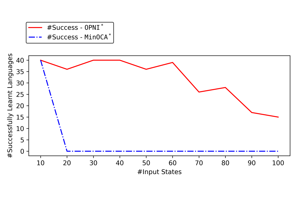
All the experiments were performed on an Apple M1 chip with 8GB of RAM. We implemented the proposed method (OCA-L^∗) in Python for droca and then for the special case of voca ³³3The implementations of OCA-L^∗ for droca, OCA-L^∗ and MinOCA for voca, the datasets used, and the complete results generated are available at [9]. The implementation of MinOCA for droca is provided in [8]. In Figure 3(a) (resp. Figure 4(a)), the total number of languages is out of 400 (resp. 40) for each input size because, for every number of states, we generated 400 (resp. 40) random droca (resp. voca) for input alphabet sizes 2, 3, 4, and 5; to keep the visualization simple, we omitted the z-axis for alphabet size and instead aggregated the number of successfully learnt languages across all alphabet sizes for each input size – this approach is used consistently across all graphs.

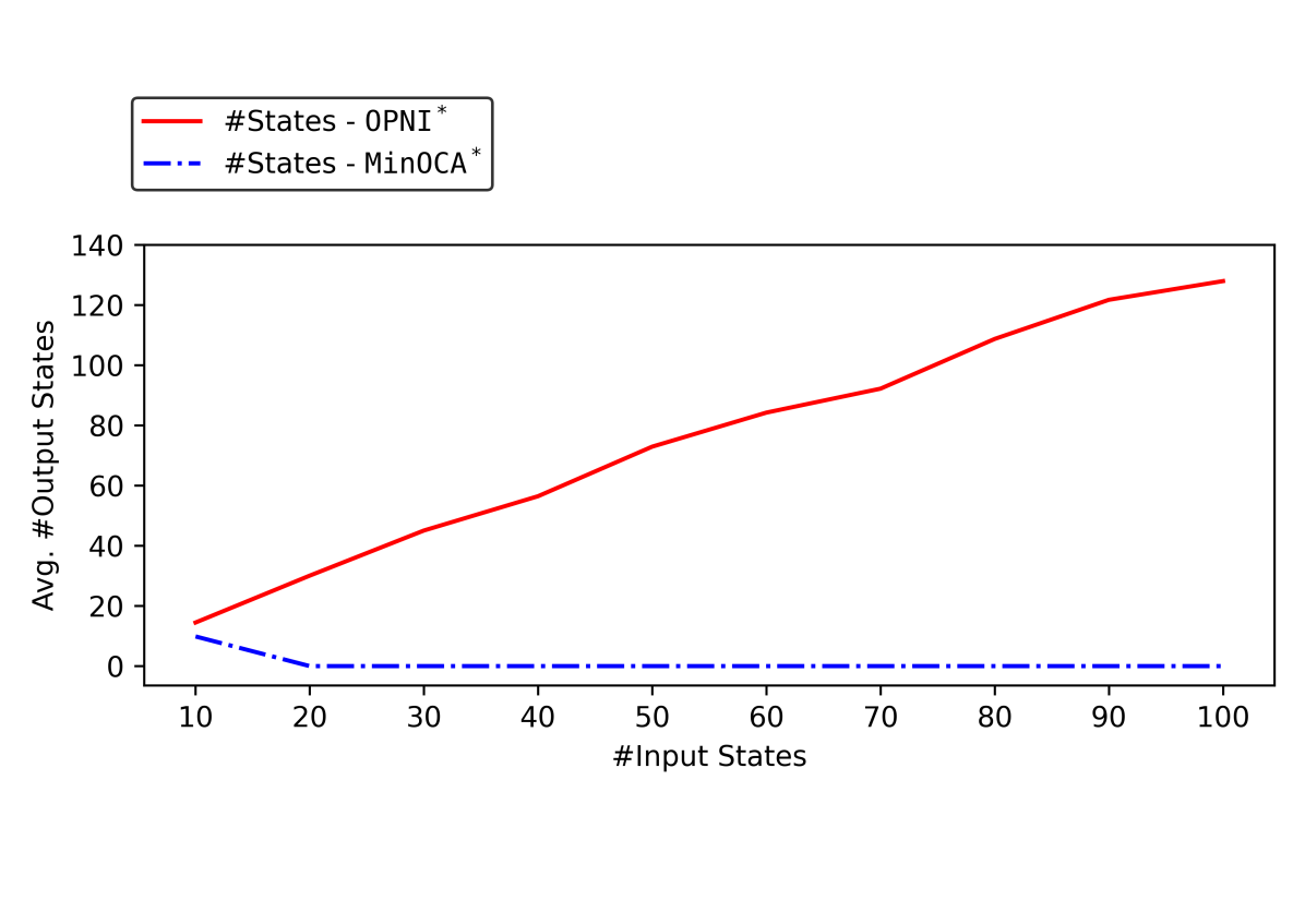
1. Evaluating the performance OCA-L^∗ and MinOCA on Dataset₁: We first compare the performance of OCA-L^∗ for droca with that of MinOCA [11]. A timeout of $5$ minutes was allotted for both MinOCA and OCA-L^∗ for learning each droca. If the procedure times out, we discard that input and process the next one. The number of languages successfully learnt by OCA-L^∗ and MinOCA for different input sizes is depicted in Figure 3(a). The proposed method outperforms MinOCA in terms of the number of successfully learnt languages within the given timeout as the number of states increases. The averages presented in the remaining graphs are computed using only those languages that were successfully learnt. Note that the y-values for MinOCA remain zero in all graphs for input sizes with more than $15$ states, as it fails to learn any language within the specified timeout.

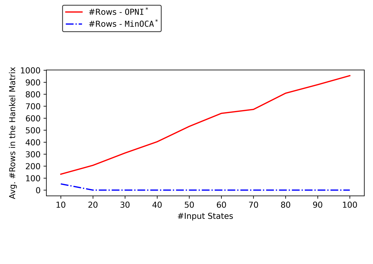
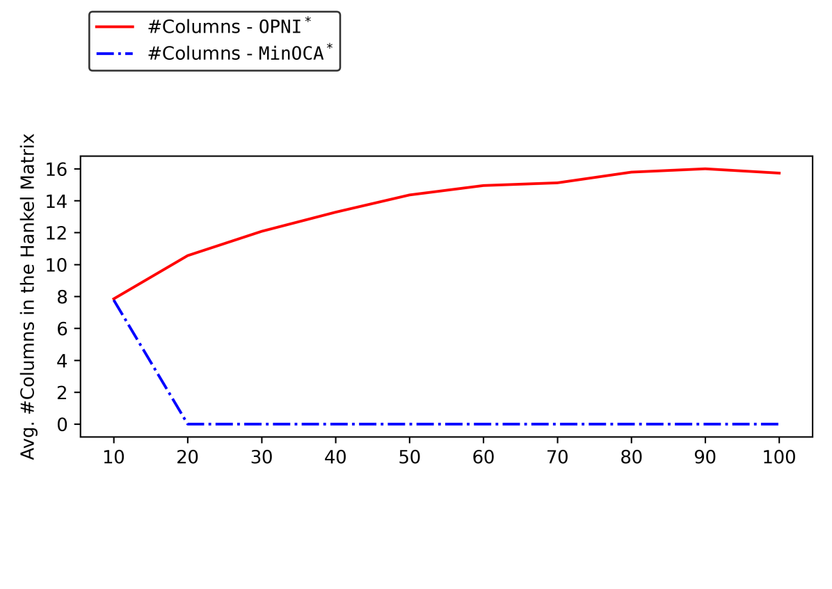
Figure 3(b) shows the average length of the longest counter-example. Since MinOCA guarantees learning a minimal counter-synchronous droca, whereas OCA-L^∗ provides no such guarantee, the droca learnt by OCA-L^∗ typically has more states. Consequently, the length of the counterexamples also tends to be longer for OCA-L^∗. Figure 3(c) shows the average number of states in the learnt droca. MinOCA learns a minimal counter-synchronous droca equivalent to the input. However, the droca learnt by OPNI is equivalent and counter-synchronous with respect to the input, but not minimal. Figure 3(d) shows the average number of equivalence queries used for successfully learning the input droca. We also add in Appendix B Figure 9(a) and Figure 9(b) the average number of rows and columns in the final observation table.

Note that OCA-L^∗ is a semi-algorithm; its termination is not guaranteed. However, our experimental results on randomly generated benchmarks show that it works well in practice.

2. Evaluating the performance OCA-L^∗ and MinOCA on Dataset₂: We now compare the performance of OCA-L^∗ for voca with that of MinOCA [11]. We note that OCA-L^∗ for voca is faster compared to OCA-L^∗ for droca. This is mainly due to the following two reasons:

1. 1.

   faster algorithm for checking equivalence of voca, and

2. 2.

   the input alphabet itself determines the counter actions, and therefore, step 2 and step 3 of Algorithm 2 can be skipped while passive learning voca.

A similar modification of MinOCA for voca was also implemented. A timeout of $20$ minutes was allotted for both procedures for learning each voca. If the procedure times out, we discard that input and process the next one. The number of voca languages successfully learnt by OCA-L^∗ for different input sizes is shown in Figure 4(a). We observe that OCA-L^∗ is able to learn close to $50\%$ of voca of $100$ states. However, it was not able to learn any voca with more than $20$ states. The averages presented in the remaining graphs are computed using only those languages that were successfully learnt. Note that the y-values for MinOCA remain zero in all graphs for input sizes with more than $20$ states, as it fails to learn any language within the specified timeout.

The results of our experiments are shown in Figure 4. Figure 4(b) shows the average length of the longest counter-example. Figure 4(c) shows the average number of states in the learnt voca. Figure 4(d) shows the average number of equivalence queries used for successfully learning the input voca. In this case also, the voca learnt by MinOCA is minimal, whereas the one learnt by OCA-L^∗ is not. Figure 10(a) and Figure 10(b) (see Appendix B) show the average number of rows and columns in the final observation table.

References

- [1] Rajeev Alur and P. Madhusudan. Visibly pushdown languages. In STOC, pages 202–211. ACM, 2004. doi:10.1145/1007352.1007390.
- [2] Rajeev Alur and P. Madhusudan. Adding nesting structure to words. J. ACM, 56(3):16:1–16:43, 2009. doi:10.1145/1516512.1516518.
- [3] Dana Angluin. Learning regular sets from queries and counterexamples. Inf. Comput., 75(2):87–106, 1987. doi:10.1016/0890-5401(87)90052-6.
- [4] Stanislav Böhm and Stefan Göller. Language equivalence of deterministic real-time one-counter automata is nl-complete. In MFCS, volume 6907 of Lecture Notes in Computer Science, pages 194–205. Springer, 2011. doi:10.1007/978-3-642-22993-0_20.
- [5] Véronique Bruyère, Guillermo A. Pérez, and Gaëtan Staquet. Learning realtime one-counter automata. In TACAS (1), volume 13243 of Lecture Notes in Computer Science, pages 244–262. Springer, 2022. doi:10.1007/978-3-030-99524-9_13.
- [6] Daniele Dell’Erba, Yong Li, and Sven Schewe. DFAMiner: Mining minimal separating dfas from labelled samples. In FM (2), volume 14934 of Lecture Notes in Computer Science, pages 48–66. Springer, 2024. doi:10.1007/978-3-031-71177-0_4.
- [7] Amr F. Fahmy and Robert S. Roos. Efficient learning of real time one-counter automata. In ALT, volume 997 of Lecture Notes in Computer Science, pages 25–40. Springer, 1995. doi:10.1007/3-540-60454-5_26.
- [8] Prince Mathew. MinOCA, January 2025. doi:10.5281/zenodo.14604419.
- [9] Prince Mathew. OCA-L*, October 2025. doi:10.5281/zenodo.17310292.
- [10] Prince Mathew, Vincent Penelle, and A. V. Sreejith. Learning deterministic one-counter automata in polynomial time. In LICS, pages 444–457, 2025.
- [11] Prince Mathew, Vincent Penelle, and A. V. Sreejith. Learning real-time one-counter automata using polynomially many queries. In TACAS (1), volume 15696 of Lecture Notes in Computer Science, pages 276–294. Springer, 2025. doi:10.1007/978-3-031-90643-5_14.
- [12] Daniel Neider and Christof Löding. Learning visibly one-counter automata in polynomial time. Technical Report, RWTH Aachen, AIB-2010-02, 2010.
- [13] José Oncina and Pedro Garcia. Inferring regular languages in polynomial updated time. In Pattern recognition and image analysis: selected papers from the IVth Spanish Symposium, pages 49–61. World Scientific, 1992.
- [14] Leslie G. Valiant and Mike Paterson. Deterministic one-counter automata. J. Comput. Syst. Sci., 10(3):340–350, 1975. doi:10.1016/S0022-0000(75)80005-5.
Appendix A Section 4. OCA-L∗: OPNI-guided active learning procedure for OCA