New Greedy Spanners and Applications

Popova, Elizaveta; Tzalik, Elad

doi:10.4230/LIPIcs.ITCS.2026.107

New Greedy Spanners and Applications

Elizaveta Popova Weizmann Institute of Science, Rehovot, Israel Elad Tzalik

Weizmann Institute of Science, Rehovot, Israel

Abstract

We present a simple greedy procedure to compute an $(\alpha,\beta)$ -spanner for a graph $G$ . We then show that this procedure is useful for building fault-tolerant spanners, as well as spanners for weighted graphs.

Our first main result is an algorithm that, given a multigraph $G$ , outputs an $f$ edge fault-tolerant $(k,k-1)$ -spanner $H$ of size $O(fn^{1+\frac{1}{k}})$ which is tight. To our knowledge, this is the first tight result concerning the price of fault tolerance in spanners which are not multiplicative, in any model of faults.

Our second main result is a new construction of a spanner for weighted graphs. We show that any weighted graph $G$ has a subgraph $H$ with $O(n^{1+\frac{1}{k}})$ edges such that any path $P$ of hop-length $\ell$ in $G$ has a replacement path $P^{\prime}$ in $H$ of weighted length $\leq w(P)+(2k-2)w^{(1/2)}(P)$ where $w(P)$ is the total edge weight of $P$ , and $w^{(1/2)}$ denotes the sum of the largest $\lceil\frac{\ell}{2}\rceil$ edge weights along $P$ . Moreover, we show such approximation is optimal for shortest paths of hop-length $2$ . To our knowledge, this is the first construction of a “spanner” for weighted graphs that strictly improves upon the stretch of multiplicative $(2k-1)$ -spanners for all non-adjacent vertex pairs, while maintaining the same size bound.

Our technique is based on using clustering and ball-growing, which are methods commonly used in designing spanner algorithms, to analyze simple greedy algorithms. This allows us to combine the flexibility of clustering approaches with the unique properties of the greedy algorithm to get improved bounds. In particular, our methods give a very short proof that the parallel greedy spanner adds $O(kn^{1+\frac{1}{k}})$ edges, improving upon known bounds.

Keywords and phrases:

Graph Spanners, Greedy Algorithms

Funding:

Elad Tzalik: Supported by the Adams Fellowship Program of the Israel Academy of Sciences and Humanities.

Copyright and License:

2012 ACM Subject Classification:

Mathematics of computing

\rightarrow

Graph algorithms

Acknowledgements:

We are deeply grateful to Merav Parter for her invaluable guidance, encouraging this collaboration, and suggesting the problem of constructing better FT

(\alpha,\beta)

-spanners. We thank Asaf Petruschka for clarifying the connection between the bounded-degree fault model and the parallel greedy spanner, and we thank Nathan Wallheimer and Ron Safier for useful discussions.

DOI:

10.4230/LIPIcs.ITCS.2026.107

Event:

17th Innovations in Theoretical Computer Science Conference (ITCS 2026)

Editor:

Shubhangi Saraf

Series and Publisher:

Leibniz International Proceedings in Informatics, Schloss Dagstuhl – Leibniz-Zentrum für Informatik

1 Introduction

Let $G$ be an $n$ -vertex weighted graph. A spanner of $G$ is a subgraph that approximately preserves distances. Formally, a subgraph $H$ is a $t$ -spanner of $G$ if $\mathrm{dist}_{H}(u,v)\leq t\cdot\mathrm{dist}_{G}(u,v)$ for all $u,v\in V$ (where $\mathrm{dist}_{X}$ denotes the shortest path distance in a graph $X$ ). Since their introduction by Peleg and Ullman [41] and Peleg and Schäffer [39], spanners have been found to be extremely useful for a wide variety of applications, including network tasks like routing and synchronization [40, 44, 21, 22, 41], preconditioning linear systems [27], distance estimation [45, 7], and many others. The first tight construction of spanners was given by [5], which proved that any graph admits a $(2k-1)$ -spanner with $O(n^{1+\frac{1}{k}})$ edges, which is best possible¹¹1The $O(n^{1+\frac{1}{k}})$ upper bound is tight assuming the girth conjecture of Erdős. Nevertheless, the algorithm of [5] is optimal unconditionally..

The foundational work of Althöfer et al. [5], focuses on providing a stretch $(2k-1)$ for adjacent pairs of vertices, and highlights that graphs of girth $>2k$ are a bottleneck for such sparsification. To handle these bottlenecks, much work has focused on $(\alpha,\beta)$ -spanners.

Definition 1 (( $\alpha,\beta$ )-spanner).

Let $G=(V,E)$ be a graph. A subgraph $H\subseteq G$ is called an $(\alpha,\beta)$ -spanner of $G$ if for all $u,v\in V$ ,

\mathrm{dist}_{H}(u,v)\;\leq\;\alpha\cdot\mathrm{dist}_{G}(u,v)+\beta.

When $\beta=0$ we call $H$ a multiplicative spanner, and when $\alpha=1$ we call it an additive spanner.

Intuitively, $(\alpha,\beta)$ -spanners have effectively multiplicative stretch $\alpha$ for vertices that are far apart in $G$ , while $\beta$ masks the local bottlenecks such a graph may have – in order to achieve an upper bound $O(n^{1+\frac{1}{k}})$ on the size of the spanner. The first indication that one can provide improved stretch for distant vertices is the seminal work of Elkin and Peleg [30]. In [30] the authors constructed $(1+\varepsilon,\beta)$ spanners of size $O_{\varepsilon,k}(n^{1+\frac{1}{k}})$ edges and $\beta=O\left(\frac{\log(k)}{\varepsilon}\right)^{\log k}$ for every integer $k$ and $\varepsilon\in(0,1)$ , as well as a $(k-1,O(k))$ -spanner. This sparked many follow-up works to investigate the tradeoffs of size, distance and stretch achievable in graph sparsification and in particular the $(k,k-1)$ spanner of Baswana et al. [6], the spanner of Thorup and Zwick [46], and many additional works e.g. [17, 9, 28].

In real-world scenarios, spanners are frequently employed in systems whose components are susceptible to occasional breakdowns. It is therefore desirable to have spanners possessing resilience to such failures, leading to the notion of fault-tolerant (FT) spanners. Two extensively studied types of faults are edge faults and vertex faults. Spanners in the edge/vertex fault-tolerant (E/VFT) settings are defined as follows:

Definition 2 (E/VFT Spanner).

An $f$ -EFT (VFT) $(\alpha,\beta)$ -spanner of $G$ is a subgraph $H$ such that for every set $F$ of at most $f$ edges (vertices) in $G$ , it holds that $H-F$ is an $(\alpha,\beta)$ -spanner of $G-F$ .

E/VFT spanners have received major interest in recent years; see, e.g., [18, 23, 10, 14, 24, 11, 12, 36] and references therein. The current state of affairs is that multiplicative FT spanners are well understood; this is reflected by essentially tight bounds on the size of fault tolerant spanners in case of vertex faults [14, 36], edge faults [12], bounded degree faults [13], and color faults [42, 37].

In contrast, the right size bounds required from an $f$ -FT $(\alpha,\beta)$ spanners is poorly understood, and no tight bounds are known for given $(\alpha,\beta)$ that improve the stretch obtained by the multiplicative $f$ -FT $(2k-1)$ -spanner in any FT model. The work of [15] studied FT additive and $(\alpha,\beta)$ -spanners and constructed $f$ -EFT $(k+\varepsilon,k-1)$ -spanners with $O\left(f\cdot\left(\frac{(k-1)}{\varepsilon}\right)^{2f}n^{1+\frac{1}{k}}\right)$ many edges. An alternative construction may be given using the method of Dinitz and Krauthgamer [23] to obtain $f$ -EFT $(k,k-1)$ -spanners with $\tilde{O}\left(f^{3}n^{1+\frac{1}{k}}\right)$ many edges. Finally, one may use an $f$ -EFT $k$ -spanner which can be done in $O(fn^{1+(1/\lceil k/2\rceil)})$ for multigraphs [18, 14], and $O(kf^{\frac{1}{2}}n^{1+(1/\lceil k/2\rceil)}+fn)$ for simple graphs. Moreover, each of the aforementioned results, improves upon the others for some range of $f$ , which sums up into an unclear picture on the “overhead” one needs to pay for faults in $(\alpha,\beta)$ -spanners. Meanwhile, for lower bounds, a folklore lower bound, a multigraph with $\Omega(fn^{1+\frac{1}{k}})$ edges and no proper $f$ -EFT $(k,k-1)$ -spanner, is known²²2The lower bound is conditional on the Erdős girth conjecture. The conjecture states that for all integers $k$ there exist an $n$ node graph with $\Omega(n^{1+\frac{1}{k}})$ edges and girth $>2k+1$ . It is common in the area of FT spanners to base lower bounds on the Erdős girth conjecture, see e.g. [10, 13, 42] and reference therein..

Our first main result is clarifying the picture for $f$ -EFT, $(k,k-1)$ -spanners in multigraphs, by giving a tight upper bound matching the best known lower bound, resolving a long-standing gap, and improving the $\tilde{O}(f^{3})$ dependency on $f$ by the Dinitz-Krauthgamer approach, to a tight $O(f)$ overhead. We prove:

Theorem 3.

Let $G$ be a multigraph and let $k,f\in\mathbb{N}$ . Then:

1.

Existence. There exists an $f$ -EFT $(k,k\!-\!1)$ -spanner $H$ of $G$ with $O\!\big(f\,n^{1+1/k}\big)$ edges.
2.

Construction. There is a polynomial-time algorithm that outputs an $f$ -EFT $(k,k\!-\!1)$ -spanner $H$ of $G$ with $O\!\big(kf\,n^{1+1/k}\big)$ edges.

We highlight that spanners are never used with $k$ larger than $O(\log n)$ , since the additional stretch does not bring additional sparsity. On the other hand, the fault parameter $f$ can be significantly larger, for example polynomial in $n$ . In light of this, the improvement of Theorem 3 on the current known bounds is substantial, and achieves stretch of an $(k,k-1)$ -spanner under faults, with the same upper bound formerly known only for the weaker multiplicative $(2k-1)$ fault tolerant spanners, see Table 1.

We emphasize two natural reasons to focus on multigraphs: (1) We believe they are more natural than simple graphs in the presence of faults. This is reflected e.g. in the fact that when adding colors to the edges and allowing color faults, the bounds for FT-spanners in multigraphs do not change. On the other hand, when introducing color faults to a simple graph one gets exactly the same behavior as multigraphs, e.g. the upper/lower bounds for edge-color-fault tolerant spanners in simple graphs jumps to $\Omega(fn^{1+\frac{1}{k}})$ , matching the bound for edge faults/ edge-color faults in multigraphs³³3See [42] for a more detailed discussion on the best bounds on the various fault models, and the effect of introducing colors.. (2) Even for the well-studied multiplicative EFT spanners, tight lower bounds are known for multigraphs but not for simple graphs, see [12].

Table 1: Size bounds for

f

-EFT

(\alpha,\beta)

-spanners on multigraphs.

$(\alpha,\beta)$	Size bound	Ref.
$(k+\varepsilon,k-1)$	$O\left(f\cdot\left(\frac{(k-1)}{\varepsilon}\right)^{2f}fn^{1+\frac{1}{k}}\right)$	[15]
$(k,k-1)$	$\tilde{O}\left(f^{3}n^{1+\frac{1}{k}}\right)$	[23]
$(k,0)$	$O(fn^{1+(1/\lceil k/2\rceil)})$	[18, 14]
$(2k-1,0)$	$O(fn^{1+1/k})$	[18, 14]
$(k,k-1)$	$O(fn^{1+\frac{1}{k}})$	new

Our second main result concerns weighted graphs. Spanners are often used to compress metric spaces that correspond to weighted input graphs, see e.g. [16, 25, 34, 43]. Standard multiplicative spanners can handle weights easily, yet obtaining different better stretches for further pairs is not as obvious. The work of Cohen [20] constructed weighted $(1+\varepsilon,\beta)$ spanners where the additive term corresponds to a $+\beta\cdot w_{max}(G)$ approximation of the distance on top of the multiplicative stretch, where $w_{max}(G)$ denotes the maximum edge weight over all edges in $G$ , which was then improved by [26]. In recent years, there has been a renewed and growing interest in understanding spanners for weighted graphs. The work of [28] achieved constructions of weighted $(\alpha,\beta)$ spanners with local stretch, meaning that $w_{max}(G)$ is replaced by the maximum $w_{max}(P)$ , which stands for the maximum edge weight along a shortest path $P$ between nodes. This was later further studied for additive stretch in a sequence of works obtaining essentially tight results [4, 29, 2, 33].

While for unweighted graphs, an $(\alpha,\beta)$ spanner has a better stretch than an $(\alpha^{\prime},\beta^{\prime})$ spanner with $\alpha<\alpha^{\prime}$ for far enough vertex pairs, this is not necessarily the case in the weighted setting as the $+\beta w_{max}$ term can significantly outweigh the weight of the path. In particular, while the line of works [4, 29, 2, 33] gives tight bounds for additive spanners, such spanners may require $\Omega(n^{\frac{4}{3}-\varepsilon})$ edges for any $\epsilon>0$ by the seminal work of Abboud and Bodwin [1]. The state of weighted spanners with $O(n^{1+\frac{1}{k}})$ edges and local stretch guarantee is less understood, with essentially a single construction of Elkin Gitlitz and Neiman [28] of a weighted $\left(O(1),k^{O(1)}\right)$ - spanner with $O(n^{1+\frac{1}{k}})$ edges. Our second result aims to fill in two gaps that weighted $\left(O(1),k^{O(1)}\right)$ - spanner with $O(n^{1+\frac{1}{k}})$ have: (1) the bound is ineffective for paths $P$ of hop length $O(k^{O(1)})$ , in the sense that a $(2k-1)$ multiplicative spanner produces a better stretch, and (2) In case of very irregular weights in $G$ , the $+k^{O(1)}w_{max}(P)$ term may significantly outweigh the constant multiplicative stretch guaranteed. We complement their result by filling these gaps. We show an algorithm that takes a graph $G$ and returns a subgraph $H$ of size $O(n^{1+\frac{1}{k}})$ which strictly improves over the stretch of the multiplicative greedy algorithm for all non-adjacent vertices, and obtains optimal approximation for vertices whose shortest path consists of two edges. Given a path $P$ of length $\ell$ , let $w(P)$ denote the sums of weights along the path, i.e. $w(P)=\sum_{e\in P}w(e)$ , and similarly define $w^{(1/2)}(P)$ the sum of the $\lceil\frac{\ell}{2}\rceil$ highest weights along the path $P$ . We prove:

Theorem 4.

For every weighted graph $G$ , there exists a subgraph $H$ with $O\!\big(n^{1+1/k}\big)$ edges such that for every pair $x, y$ joined by a path $P$ in $G$ ,

\mathrm{dist}_{H}(x,y)\;\leq\;w(P)+(2k-2)\,w^{(1/2)}(P).

Moreover, for shortest paths of hop-length $2$ this bound is best possible.

To our knowledge, such tight bounds in Theorem 4 were not known, even in the unweighted setting. The work of Baswana et al. [6] achieves an upper bound of $O(kn^{1+\frac{1}{k}})$ for $(k,k-1)$ spanners while the work of Parter [35] achieved stretch $k$ for vertices at distance $2$ (in the unweighted case) and size $O(k^{2}n^{1+\frac{1}{k}})$ . Nevertheless in our viewpoint handling weighted graphs is the more interesting part of Theorem 4, whereas the $k$ factors is a secondary improvement.

Finally, we show that our technique is robust and useful for analyzing other variants of the greedy spanner. The parallel greedy spanner algorithm, introduced by Haeupler, Hershkovitz and Tan [31], is a variant of the standard greedy algorithm of [5] for computing a $(2k-1)$ spanner, where instead of considering an edge $e_{i}$ at the $i^{th}$ step, a set of edges $M_{i}$ which forms a matching is being considered, and each edge of $M_{i}$ decides for itself greedily if it could be discarded from $G$ , or if it will be added to $H$ (the decision is done by checking for $e=\{u,v\}$ if $\mathrm{dist}_{H_{i}}(u,v)>2k-1$ , where $H_{i}$ is the spanner before $M_{i}$ was considered). The parallel greedy spanner algorithm appears in relation to later works on length-constrained expanders and routing algorithms, see [19, 32]. The main result of [31] is that the parallel greedy algorithm adds at most $O(n^{1+O(\frac{1}{k})})$ edges overall, which was later improved to $O(k)^{k}\cdot O(n^{1+\frac{1}{k}})$ by Bodwin, Haeupler and Parter [13]. Both papers are technically heavy, with [31] “length-constrained” expander decomposition machinery, and [13] used the counting/dispersion approach of [12] together with a complex choice of paths to count over⁴⁴4The work of [13] does not specifically target parallel greedy spanners but the more challenging bounded-degree FT-spanners, yet their results imply upper bounds on the output size of the parallel greedy spanner.. We show that by applying the tools we develop in this work, one gets an elementary analysis (at most two pages) of the following improved bound:

Proposition 5.

The output of the parallel greedy spanner algorithm with stretch parameter $(2k-1)$ has $O(kn^{1+\frac{1}{k}})$ many edges, and arboricity $O(kn^{1/k})$ .

1.1 Technical Overview

The starting point of this work, as well as a central component of the FT-spanner we construct, is a new greedy algorithm we introduce and analyze.

The Greedy $d\to r$ Spanner Algorithm

Our goal will be to study the following problem: given a graph $G$ and integers $d, r$ , find a sparse subgraph $H$ , such that vertices at distance exactly $d$ in $G$ are at distance $\leq r$ in $H$ :

Definition 6 ( $d\to r$ spanner).

Let $d, r$ be natural numbers. We say that a subgraph $H$ of $G$ is a $d\to r$ spanner of $G$ if $\forall x,y\in V$ :

\mathrm{dist}_{G}(x,y)=d\implies\mathrm{dist}_{H}(x,y)\leq r

We highlight that this definition is similar to the definition of $f(d)$ -spanner appearing in many works and refer the reader to the survey [3] and references therein. Given $f:\mathbb{N}\to\mathbb{N}$ an $f(d)$ spanner $H$ of $G$ is a subgraph $H$ which is a $d\to f(d)$ spanner for all $d$ , hence the main distinction in our approach is specializing only in fixed $d,f(d)$ . $d\to r$ spanners can be thought of as building blocks for $(\alpha,\beta)$ spanners in particular we highlight the work of Parter [35] giving an almost tight construction of $2\to 2k$ spanners, and the later work of Parter and Ben-Levy [9] which constructs $k^{\varepsilon}\to O_{\varepsilon}(k)$ spanners with $O_{k,\varepsilon}(n^{1+\frac{1}{k}})$ edges for $0<\varepsilon<1$ . We emphasize that the union of a few $d\to r$ spanners usually make an $(\alpha,\beta)$ -spanner and in particular it is folklore (and easy to prove) that a union of a $1\to 2k-1$ and a $2\to 2k$ spanner of a graph $G$ , always produces a $(k,k-1)$ spanner. We will construct spanners by analyzing the following simple greedy $d\to r$ spanner algorithm:

Algorithm 1 Greedy

d

\to

r

Spanner

(G,d,r)

.

Large Cliques in the Output of the $d\to r$ Greedy Algorithm

While the high girth of the greedy spanner of [5] is a main feature used in most works, the output of the $d\to r$ greedy algorithm for $d>1$ may have very small girth. To demonstrate this, we show that the output of the $2\to 2k$ greedy algorithm does not necessarily have high girth, e.g. it can have a clique of size $\sqrt{n}$ . Consequently, getting a meaningful size bound for the output of the algorithm requires more than just girth.

Claim 7.

There exists a graph $G$ on $n$ vertices and an order of the $2$ -paths in it such that when the greedy $2\to 2k$ algorithm processes the paths in order, the output has a clique of size $\Omega(\sqrt{n})$ .

Proof.

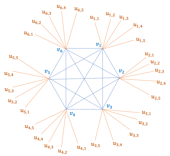
Set $n=t^{2}$ , and consider a clique of $t$ vertices $v_{1},...,v_{t}$ . Connect each $v_{i}$ to $t-1$ other vertices $u_{i,1},...,u_{i,t-1}$ , where all $u_{i,j}$ are distinct and so each a leaf in the resulting graph, see Figure 1. Consider the following sequence of $2$ -paths: $((v_{i+j},v_{i},u_{i,j}))_{i\in[t],j\in[t-1]}$ in the lexicographical order of $(i,j)$ , with the indices of $v_{i}$ considered modulo $t$ .

By construction, each new path introduces a fresh leaf, ensuring it will be kept by the greedy algorithm, forcing all clique edges into the output (see Figure 1). This shows that the greedy algorithm is forced to include every clique edge. The union of these paths contains the entire graph, and in particular, a $t$ -clique. $\hfill\vartriangleleft$

Refer to caption — Figure 1: A big clique in the output of the $2\to 2k$ greedy spanner.

The Clustered vs. Nearby Process

To bypass the lack of high girth we take a new approach, based on clustering see e.g [30, 6, 8, 17, 9]. A central definition we use is that of a clustered vertex in a graph: a vertex $v$ is $\ell$ clustered in a graph $G$ with $n$ nodes if for all $i\leq\ell$ , $|B_{G}(v,i)|\geq n^{i/k}$ ⁵⁵5Notice the definition of clusters depend on $n$ and $k$ , though we omit $k$ from the definition for simplicity, as it is fixed throughout the paper.. This definition is inspired by the new “local” viewpoint of the Baswana-Sen algorithm of [37]. We show that adding an edge between relatively far vertices in a graph helps them become more clustered, which is captured by the following key lemma:

Lemma 8 (Neighborhood exchange lemma).

Let $(u,v)$ be vertices in a graph $H$ , and assume that $\mathrm{dist}_{H}(u,v)>s$ . Let $H^{\prime}=H\cup\{u,v\}$ Then for every $\ell\leq\lceil\frac{s}{2}\rceil-1$ :

(a)

$B_{H}(u,\ell)\cap B_{H}(v,\ell+1)=\emptyset$ .
(b)

$B_{H^{\prime}}(u,\ell)\subseteq B_{H^{\prime}}(v,\ell+1)$ .

The merit of the lemma above is that it implies good bounds on the following algorithm we introduce, called the Clustered vs. Nearby Process: For an input graph $G$ , initialize an empty graph $H$ and iteratively consider an edge $e\in G$ , and add $e$ to $H$ if: (1) The endpoints of $e$ are at mutual distance $>s$ in $H$ , and (2) one of $e$ ’s endpoints is not $\lceil\frac{s}{2}\rceil$ clustered in $H$ . Using the lemma we show that this process adds only $O(sn^{1+\frac{1}{k}})$ edges where $k$ is the parameter of clustering. In particular if one inserts to this process the edges of a graph $G$ , one obtains a graph $H$ as output, together with the following invariant which is often critical in clustering methods⁶⁶6See e.g. the local analysis of the Baswana-Sen algorithm in [37].: for every $\{u,v\}=e\in E(G)-E(H)$ either (1) $u, v$ are both $\lceil\frac{s}{2}\rceil$ clustered or (2) $\mathrm{dist}_{H}(u,v)\leq s$ ⁷⁷7One can also extend this process naturally to weighted graphs, which we use in the main result of Section 4. We then apply this lemma to an analogous parallel clustered vs. nearby process – to obtain essentially tight bounds for parallel greedy spanners. The size bound of $O(sn^{1+\frac{1}{k}})$ on the number of edges added by the process has a factor $s$ which is present because the analysis of clustering using Lemma 8 goes in $s$ rounds. It turns out that sequential algorithms enjoy a better upper bound than the one achieved by this round-by-round clustering. In Section 2 we prove that when edges in the nearby vs clustered process are added sequentially, the number of edges added by this process is $O(n^{1+\frac{1}{k}})$ . We view the process as a greedy way to achieve clustering, and believe it will find applications in future work.

Obtaining Tight Bounds for the $2\to 2k$ Greedy Spanner

Our approach is based on combining the clustering ideas formerly described with a “path-buying” inspired algorithm, describing how distances shrink throughout the algorithm, together with an extra step we call lateral clustering. We consider the paths $P_{1},\ldots,P_{t}$ , with $P_{i}=(x_{i},m_{i},y_{i})$ added by the $2\to 2k$ greedy algorithm, in their order. For each $P_{i}$ we consider the pair $(x_{i},m_{i})$ which was at distance $>k$ before adding $P_{i}$ to the graph (such a pair must exist by the triangle inequality), we assume without loss of generality this pair is $(x_{i},m_{i})$ (otherwise reverse the path) and call it the $i^{th}$ distant pair. Concretely if $x_{i}$ or $m_{i}$ is not $\lceil\frac{k}{2}\rceil$ -clustered, we can “charge” adding $P_{i}$ as the addition of an edge to the clustered vs nearby process with distance parameter $k$ – as the sequential process adds $O(n^{1+\frac{1}{k}})$ edges, there are only $O(n^{1+\frac{1}{k}})$ paths with a distant pair with both endpoints not $\lceil\frac{k}{2}\rceil$ -clustered.⁸⁸8In other words, we use a moderate girth $>k+1$ subgraph for the analysis of the clustering that occur during the greedy $2\to 2k$ algorithm. E.g. in Figure 1 the orange edges are distant and contribute to the clustering of their endpoints, while the blue edges of the clique are typically not distant and do not contribute to clustering via the clustered vs nearby process, nevertheless we can still use such paths for clustering in a more intentional way, we describe now.

The rest of the paths have distant pairs which are both already $\lceil\frac{k}{2}\rceil$ -clustered, let $P_{i}$ be such path. If $y_{i}$ was also $\lceil\frac{k}{2}\rceil$ -clustered we will be done by a “path-buying” like argument (Originally appearing in [6]) – we can show that the $\Omega(n^{\frac{k-1}{k}})$ pairs of vertices in $B_{H}(x_{i},\lfloor\frac{k}{2}\rfloor)\times B_{H}(y_{i},\lceil\frac{k}{2}\rceil)$ are at distance $>k$ before adding $P_{i}$ but $\leq k$ after adding $P_{i}$ , as this can happens at most once for a pair of vertices, and as there are $O(n^{2})$ pairs of vertices this will apply the desired upper bound for such paths. While on a high level, the approach above describes well the main ideas that go into the proof, unfortunately it does not work as stated – there is no guarantee that $y_{i}$ is $\lceil\frac{k}{2}\rceil$ or even $1$ -clustered! To handle this, the analysis requires an additional technical step which we call “lateral” clustering. In the lateral clustering step we analyze the effect of adding $P_{i}$ on the size of the $\lceil\frac{k}{2}\rceil$ -ball around $y_{i}$ and divide into the following cases: (1) Most vertices of the $(\lceil\frac{k}{2}\rceil-1)$ -ball around $m_{i}$ were initially (before adding $P_{i}$ ) at distance $>\lceil\frac{k}{2}\rceil$ from $y_{i}$ – in this case we still get a significant increase for the size of $B_{H}(y_{i},\lceil\frac{k}{2}\rceil)$ by adding $P_{i}$ , hence the number of steps for which such paths can increase the size of a $\lceil\frac{k}{2}\rceil$ around $y_{i}$ until it has a ball of size $\geq n^{\frac{\lceil k/2\rceil}{k}}$ is $O(n^{1+1/k})$ getting us back to the path-buying type argument, as if $y_{i}$ is clustered. (2) Most vertices of the $(\lceil\frac{k}{2}\rceil-1)$ -ball around $m_{i}$ were initially (before adding $P_{i}$ ) at distance $\leq\lceil\frac{k}{2}\rceil$ from $y_{i}$ . In this case we apply a similar “path-buying” type argument for balls around $x_{i}$ and $m_{i}$ , which concludes the proof.

In the full version of the paper, we show that the greedy algorithm can also be used for other values of $d$ . We reprove a result of Ben-Levy and Parter ([9], Thm 1.2) of the existence of $\lceil\sqrt{k}\rceil\to O(k)$ spanners with $\tilde{O}(n^{1+\frac{1}{k}})$ edges, by showing the greedy algorithm with the same parameters achieves the same size bound.

1.2 Handling Faults

To handle faults, we analyze a FT-greedy algorithm, originally due to [10], adapted to the $d\to r$ spanner definition:

Definition 9 (EFT $(d\to r)$ spanners).

Let $G=(V,E)$ be a (multi)graph and $f\in\mathbb{N}$ . A subgraph $H\subseteq G$ is an $f$ -edge-fault tolerant ( $f$ -EFT) $(d\to r)$ spanner if for every $F\subseteq E$ with $|F|\leq f$ and all $x,y\in V$ :

\mathrm{dist}_{G-F}(x,y)=d\implies\mathrm{dist}_{H-F}(x,y)\leq r

We then study the FT-greedy spanner, which works as follows: For all $x, y$ go over all paths $P$ with $d$ edges between $x$ and $y$ , and add $P$ to $H$ whenever there exist a fault set $F$ of $\leq f$ edges, disjoint from $P$ , such that $\mathrm{dist}_{H-F}(x,y)>r$ . We show that the algorithm above achieves the size bounds appearing in Theorem 3.

The Blocking Set Method for $d\to r$ Spanners

In [14], Bodwin and Patel studied VFT-spanners, and prove that the $f$ -VFT $1\to 2k-1$ greedy algorithm achieves optimal size bound. To do so, define a blocking set as a collection of edge-vertex pairs, such that each short ( $\leq 2k$ ) cycle in $H$ contains one of the pairs. The FT greedy $1\to 2k-1$ algorithm naturally induces a blocking set of size $f|E(H)|$ . They then show that a graph with such blocking set has $O(f^{1-\frac{1}{k}})$ edges for the vertex fault model. On an intuitive level, a graph that admits a small blocking set is often thought of as being close to having high girth, forcing it to be sparse.

In contrast we view the output of the greedy $d\to r$ as producing graphs such that many vertices have cuts of size $f$ that substantially separate them. A spark of this viewpoint appears in [38], where a tight analysis for a FT-greedy algorithm was given by applying a “cut-based” view instead of the cycle-based view of [13]. By defining the $d\to r$ blocking set for the $d\to r$ FT-greedy algorithm, we show that the output size produced isn’t too large when compared to the standard $d\to r$ greedy spanner. We show that if $b(n)$ is a bound on the maximal number of paths added by the greedy $2\to 2k$ spanner⁹⁹9We actually need a bound for a slightly different algorithm then Algorithm 1, nevertheless this is done for technical reason elaborated in Section 5. on an $n$ -vertex graph. Then the $f$ -FT $2\to 2k$ greedy spanner adds at most $O(f\cdot b(n)+fn^{1+\frac{1}{k}})$ paths. This concludes the proof using the bounds obtained for the $2\to 2k$ spanner described previously.

The proof of the theorem above is short, and has two steps: (1) Showing that it is enough to prove the theorem when the FT algorithm adds edge-disjoint paths at each step, and (2) Showing that if the FT-greedy algorithm adds disjoint paths, then they may be thought of as “long edges” – which reduces the dependence on the fault parameter to be linear similarly to [14, 42].

In the full version of the paper we implement the modified FT-greedy approach of Dinitz and Robelle [24] to give a polynomial time construction as stated in Theorem 3.

1.3 Improving Upon Multiplicative $2k-1$ Spanners for Weighted Graphs

It is not hard to see that Theorem 4 would follow if we could show that any weighted graph $G$ has a subgraph $H$ with $O(n^{1+\frac{1}{k}})$ edges and the following property: any $2$ -path $P$ in $G$ has a replacement path $P^{\prime}$ in $H$ of weight $w(P)+(2k-2)w_{max}(P)$ which is what we achieve in Section 4. We also highlight that the section begins with a simple lower bound, Claim 32, showing that the stretch $w(P)+(2k-2)w_{max}(P)$ is the best possible stretch that can be achieved by a subgraph with $O(n^{1+\frac{1}{k}})$ edges, assuming the girth conjecture.

Following the theme presented in the paper, one may guess the following generalization of the greedy $2\to 2k$ algorithm in the spirit of [5] – go over the paths $P$ in order of weight and add each path which does not have good approximation in the current subgraph. The main difficulty in this approach stems from the following question: According to which order should $P$ be processed? The multiplicative greedy spanner scans edges, and in such case there is a natural order – order of weight. On the other hand the greedy $d\to r$ spanner for $d>1$ scans paths of length $d$ – if those were composed of weighted edges it is unclear which order to choose: maybe order the paths by maximum edge weight on the path? another natural options are the total edge weight/ a linear combination of the weights along the path. We didn’t find a single order for which the analysis goes through.

A different attempt is to use what is called $d$ -light initialization, appearing in [4, 2, 29] in the context of weighted additive spanners. $d$ -light initialization describes an initialization phase prior to running an algorithm, in which every vertex adds its $d$ lightest adjacent edges – in our case $O_{k}(n^{\frac{1}{k}})$ edges. This approach is effective in handling $k\leq 4$ but doesn’t seem to generalize to higher $k$ – the main reason is that it allows to compare weights in a very local way (around a vertex), which does not propagate to something meaningful for long enough paths. Even if one replaces the initialization phase by a clustering phase, it seems that additional structure is needed to design the algorithm.

In light of the above, we took a different approach – instead of running a greedy algorithm in some unique order, such that an analysis similar to Theorem 19 follows, we break the algorithm according to the steps in the analysis of Theorem 19, by introducing weighted notions of clustering, lateral clustering, a greedy phase, and a new “distance-reduction” phase, each with it’s own novel order. We believe that this approach can be fruitful for other constructions of spanners for weighted graphs.

We now briefly describe the phases of the algorithm, their corresponding order, and what they informally try to achieve. The spanner will be the union of all edges added in the various phases. Assume for now $k$ is even, and $R=k/2$ . The other parity of $k$ is handled similarly in Section 4.

Phase 1: Adding a Multiplicative Spanner

We begin by adding to the spanner a $(2k-1)$ multiplicative spanner with $O(n^{1+1/k})$ edges. The main reason for this phase is the following observation: every $2$ -path $P$ (in $G$ ) with an edge in the final spanner (the second edge may not be present in the final spanner) has the right stretch in the final spanner. Hence it’s enough to obtain a good stretch for $2$ -paths in $G$ with both edges not in the final spanner.

Phase 2: Greedy Clustering

We go over all edges $e$ by increasing order of weight and will run the clustered vs nearby process on all edges by order of weight and add those added by the process, which is $O(n^{1+1/k})$ edges. By the end of this phase we ensure that any edge $e=\{u,v\}$ not in the final spanner has either (1) $\mathrm{dist}_{H}(u,v)\leq kw(e)$ , or (2) that $u, v$ are clustered at the time of considering $e$ – which implies that $B_{H_{\leq w(e)}}(u,i)$ , and $B_{H_{\leq w(e)}}(v,i)$ are of size $\geq n^{\frac{i}{k}}$ , for $i\leq R$ ¹⁰¹⁰10 $H_{\leq w(e)}$ is the underlying of all edges of weight at most $w(e)$ .. In case an edge wasn’t added due to condition (2) we call this edge saturated.

It now follows that paths $P$ with two edges that weren’t included because $\mathrm{dist}_{H}(u,v)\leq kw(e)$ have good stretch already by the end of this phase. For the rest of the paths $P=(x,m,y)$ which do not meet the desired stretch by the end of phase $2$ we have (w.l.o.g) that both $x, m$ were clustered at the time (aka weight) for which the edge $\{x,m\}$ was considered in phase $2$ . This allows to add edges that improve distances between vertices, while still adding only $O(n^{1+1/k})$ edges.

Phase 3: Lateral Clustering

The lateral clustering phase is an algorithm where each vertex $y$ (independently) adds $O(n^{1/k})$ edges. For every vertex $v$ denote by $w_{v}$ to be the smallest weight of a saturated edge (see description of phase 2) incident to $v$ . Each vertex $y$ goes over it’s neighbors $u$ by order of weight $\phi=w(y,u)+(R-1)w_{u}$ and checks wether adding the edge $\{y,u\}$ substantially increases the size of the ball of radius $\phi$ around $y$ . The reason for choosing this particular order is that this way we order $y$ ’s neighbors in a monotone way according to the implied distance (to $y$ ) guarantee we can get on the vertices from $u$ ’s ball, after the edge addition.

After phase 3 the neighbors of $y$ that were not added divide into two: (type 1 neighbors) neighbors $u$ of $y$ such that at time of considering $u$ the $\phi$ -ball around $y$ was already of size $\Omega(n^{R/k})=\Omega(n^{1/2})$ , and (type 2 neighbors) neighbors $u$ such that when considering $u$ , the ball of radius $(R-1)w_{u}$ in the spanner, shares many neighbors with the ball of radius $\phi$ around $y$ .

Phase 4: Global Distance Reduction by Edges

In this phase we go over all saturated edges $e=\{u,v\}$ , that is edges that weren’t added by phase $2$ due to both endpoints being clustered (according to the corresponding weight) and reconsider adding them to the spanner – as they may create useful shortcuts for vertex pairs between their clusters. More concretely, we go over $e=(u,v)$ by order of weight and for each $e$ we check how many pairs of $B(u,Rw_{u})\times B(v,(R-1)w_{v})$ will be of distance $\leq kw(e)$ due to adding $e$ – if this quantity is $\Omega(n^{1-1/k})$ we will add $e$ to the spanner. Again this phase adds the right number of edges. The key property of this phase (together with phase 4) is that by the end of it, we have successfully handled all paths $P=(x,m,y)$ such that: (1) $(x,m)$ was saturated in phase 2, and wasn’t added during phase 4 (2) when $y$ considered $m$ in phase 3, $m$ was a type 2 neighbor when considered by $y$ .

Phase 5: Greedy Phase

The fifth and last phase is greedy, we will go over all paths $P$ that do not have the right stretch in the spanner, and if a path doesn’t satisfy the right stretch we add it. It is not hard to check that the only path $P=(x,m,y)$ that may have a bad stretch have: (1) $(x,m)$ is saturated and wasn’t added in phase 4, and (2) $m$ was a type 2 neighbor of $y$ (meaning that $y$ already has a sufficiently large ball around it). In such case, we show that many distances ( $\Omega(n^{1-1/k})$ in the set $B_{H}(x,(R-1)w(x,m))\times B_{H}(y,w(y,m)+(R-1)w_{m})$ must improve by adding the path. Still we need to make sure that every pair of vertices improve at most once. For this we choose the last order to be $2w(m,y)+(k-1)w(x,m)$ – which correspond to the distance bound of the short paths created by the greedy fixes.

1.4 Organization of the Paper

In Section 2 we set the stage and develop the key definitions and tools we need through the paper, and warm up by showing how to apply these tools to analyze the parallel greedy spanner. In Section 3 we analyze the $2\to 2k$ greedy algorithm. In Section 4 we describe and analyze the weighted spanner in Theorem 4. Section 5 concludes the construction of the $f$ -FT $(k,k-1)$ -spanner with size $O(fn^{1+\frac{1}{k}})$ .

1.5 Notations

For an unweighted graph $G$ we denote for $x,y\in V(G)$ the length of their shortest $x$ to $y$ path $P$ by $\mathrm{dist}_{G}(x,y)$ . For a path $P=(v_{1},\ldots v_{\ell+1})$ we use $x(P)$ to denote the first vertex of the path $v_{1}$ and similarly $y(P)$ denotes the last vertex on the path, and $\ell$ is the length of the path. We denote by $B_{G}(v,\ell)$ the set of vertices $u\in V(G)$ that has a path of length $\leq\ell$ to $v$ .

A weighted graph $G$ is a triple $(V,E,w)$ with $w:E\to\mathbb{R}_{>0}$ . For a path $P$ in a weighted graph we denote by $w(P)$ the sum of weights of $E(P)$ , by $w_{\max}(P)$ (resp. $w_{\min}(P)$ ) the maximum (resp. minimum) edge weight along $P$ . For a weighted graph $G$ , $\mathrm{dist}_{G}(x,y)$ denotes the minimum of $w(P)$ over all $x$ to $y$ paths in $G$ . For a weighted graph $G$ we write $G^{\circ}$ for the underlying unweighted graph of $G$ . For a threshold $\omega>0$ , let $G_{\leq\omega}$ be the subgraph of $G$ induced by edges of weight at most $\omega$ , and let $G^{\circ}_{\leq\omega}$ be its underlying unweighted graph. For two sets $A, B$ we denote $A-B$ and $A/B$ the corresponding difference set. For a set $F\subseteq E$ and graph $G=(V,E)$ we denote $G-F$ the graph $(V,E-F)$ .

2 Clustering in Changing Graphs

We now introduce tools that would be useful throughout the paper, and in particular, describe the clustered vs distant process, and prove Proposition 16.

We begin with a definition of a clustered vertex. The definition above depends on $k$ , and throughout the paper all clusters will appear with the same $k$ which will be clear from context.

Definition 10 (Clusters).

A vertex $v$ has an $\ell$ -cluster in a graph $H$ if for all $r\leq\ell$ we have $\lvert B_{H}(v,r)\rvert\geq n^{r/k}.$ If $\ell$ is maximal with this property, we say $v$ is $\ell$ -clustered.

Intuitively, being $\ell$ -clustered means that the neighborhood of a vertex grows at least polynomially fast in radius, with growth $n^{\frac{1}{k}}$ per step.

Notice that any vertex is $0$ -clustered in every graph. We also have the following observation.

Observation 11.

If a vertex $v$ is $k$ -clustered in a graph $G$ , then $\forall y\in V:\mathrm{dist}_{G}(v,y)\leq k$ .

Proof.

By definition a $k$ -clustered vertex $v$ has $|B_{G}(v,k)|\geq n^{\frac{k}{k}}=n$ . Hence $B_{G}(v,k)=V$ and the claim follows. $\hfill\blacktriangleleft$

We next restate and prove the neighborhood exchange lemma. This lemma is crucial as it shows how clustering properties propagate when adding a new edge between distant vertices.

Lemma 12 (Neighborhood exchange lemma).

Let $(u,v)$ be vertices in a graph $H$ , and assume that $\mathrm{dist}_{H}(u,v)>s$ . Let $H^{\prime}=H\cup\{u,v\}$ Then for every $\ell\leq\lceil\frac{s}{2}\rceil-1$ :

(a)

$B_{H}(u,\ell)\cap B_{H}(v,\ell+1)=\emptyset$ and $B_{H}(u,\ell+1)\cap B_{H}(v,\ell)=\emptyset$ .
(b)

$B_{H^{\prime}}(u,\ell)\subseteq B_{H^{\prime}}(v,\ell+1)$ , and $B_{H^{\prime}}(v,\ell)\subseteq B_{H^{\prime}}(u,\ell+1)$ .

Proof.

For (a), suppose $w\in B_{H}(u,\ell)\cap B_{H}(v,\ell+1)$ . Then $\mathrm{dist}_{H}(u,w)\leq\ell$ and $\mathrm{dist}_{H}(w,v)\leq\ell+1$ , so by the triangle inequality, $\mathrm{dist}_{H}(u,v)\leq 2\ell+1\leq s,$ contradicting that $\mathrm{dist}_{H}(u,v)>s$ . For (b), since $(u,v)\in H^{\prime}$ , for every $w\in B_{H^{\prime}}(u,\ell)$ we have

\mathrm{dist}_{H^{\prime}}(v,w)\leq\mathrm{dist}_{H^{\prime}}(v,u)+\mathrm{% dist}_{H^{\prime}}(u,w)\leq 1+\ell,

which implies the claim. $\hfill\blacktriangleleft$

2.1 The Clustered vs. Nearby Process

For a fixed integer $s$ (that is different in different contexts) and a subgraph $H$ of $G$ we shall call a vertex which has an $\lceil{\frac{s}{2}}\rceil$ -cluster in $H$ fully clustered in $H$ and call a pair of vertices $(u,v)$ distant if $\mathrm{dist}_{H}(u,v)>s$ . When $s$ is clear from context we simply say a vertex is fully-clustered, and that a pair of vertices is distant, according to the above.
Consider the following algorithm:

Algorithm 2 clustered-vs-nearby

(G,s,(e_{i})_{i=1}^{t})

.

We call an edge $e=\{u,v\}$ boosting if $(u,v)$ is a distant pair and either $u$ or $v$ is not fully clustered at the time of consideration. Algorithm 2 appears throughout this paper both explicitly as a step of an algorithm (also for weighted graphs, as it appears in Section 4) and implicitly as a subsequence of actions performed by the greedy algorithm that can be coupled with execution of Algorithm 2. We now state and prove an upper bound on the number of edges that can be actually added by Algorithm 2.

Proposition 13.

The number of edges added by Algorithm 2 is $O(n^{1+\frac{1}{k}})$ for any $s$ .

For the proof we will need the following:

Lemma 14.

Let $G=(V,E)$ be a graph with $n$ vertices, and $E=\{e_{1},\ldots,e_{t}\}$ with $e_{i}=\{u_{i},v_{i}\}$ . Let $G_{i}$ be the graph $(V,\{e_{1},\ldots,e_{i-1}\})$ . Assume moreover the following holds:

1.

$G$ has girth $>s+1$ .
2.

For every $i$ , either $u_{i}$ or $v_{i}$ does not have $\lceil\frac{s}{2}\rceil$ -cluster in $G_{i}$ .

Then $t=O(n^{1+\frac{1}{k}})$ .

Proof.

Let $D$ be the average degree of $G$ . Recall that we can always find an induced subgraph $G^{\prime}=(V^{\prime},E^{\prime})$ of $G$ of minimum degree $D^{\prime}$ with $\frac{D}{2}\leq D^{\prime}$ , by iteratively removing low degree vertices. We claim $D^{\prime}<n^{\frac{1}{k}}+2$ . Assume towards contradiction that $D^{\prime}\geq n^{\frac{1}{k}}+2$ . Let $e$ be the last edge from $E(G)$ appearing in $G^{\prime}$ , and $G^{\prime\prime}=(V^{\prime},E^{\prime}-e)$ , and observe that clearly we have that the minimum degree of $G^{\prime\prime}$ is at least $n^{\frac{1}{k}}+1$ . Since $G$ has girth $>s+1$ the same holds for the subgraph $G^{\prime\prime}$ . Moreover since $G^{\prime}$ has girth $>s+1$ , the BFS tree around every vertex has no collisions up to radius $\lceil\frac{s}{2}\rceil$ . We obtain that for any vertex $v\in V^{\prime},\ell\leq\lceil\frac{s}{2}\rceil$ we have

|B_{G^{\prime\prime}}(v,\ell)|\geq 1+\sum_{i=0}^{\ell-1}D^{\prime\prime}\cdot(% D^{\prime\prime}-1)^{i}\geq 1+n^{\frac{1}{k}}\sum_{i=1}^{\ell-1}n^{i/k}\geq n^% {\ell/k}.

In particular this means every vertex in $G^{\prime\prime}$ is $\lceil\frac{s}{2}\rceil$ -clustered including the endpoints of $e$ – contradiction to assumption 2 of the lemma. Hence we conclude that $\frac{D}{2}\leq D^{\prime}\leq n^{\frac{1}{k}}+2$ . As $D=\frac{2|E|}{|V|}$ we obtain $|E|=O(n^{1+\frac{1}{k}})$ . $\hfill\blacktriangleleft$

Proof of Proposition 13.

Consider the graph on vertex set $V(G)$ induced by all the edges added by Algorithm 2. We claim that this graph has girth $>s+1$ .

Assume the contrary: there is a cycle of length $\leq s+1$ . Consider the edge $e_{i}=\{u_{i},v_{i}\}$ , the last edge added by the algorithm along the cycle. All other edges of the cycle were present in $H$ at the moment when the algorithm considered $e_{i}$ and they formed a path between $u_{i}$ and $v_{i}$ , hence $\mathrm{dist}_{H}(u_{i},v_{i})\leq s$ , which contradicts condition (1) of adding $e_{i}$ .

Now we see that the sequence of edges added by Algorithm 2 satisfies the conditions of Lemma 14: the high girth condition is just shown and the non-clustered condition is implied by condition (2) of adding an edge. So the desired bound follows. $\hfill\blacktriangleleft$

Now we will state and prove a result for the parallel greedy spanner. The parallel greedy spanner is defined algorithmically as follows.

Algorithm 3 Greedy parallel

1

\to

2k-1

Spanner

(G,k,\{\mathcal{M}_{i}\}_{i=1}^{t})

.

Definition 15 (Parallel greedy $1\to 2k-1$ spanner).

In a graph $G$ on $n$ vertices fix some (ordered) sequence of matchings $\mathcal{M}_{1},...,\mathcal{M}_{t}$ . We call the output $H$ of the Algorithm 3 on input $(G,k,\{\mathcal{M}_{i}\}_{i=1}^{t})$ a parallel greedy $1\to 2k-1$ spanner of $G$ .

We shall prove the following:

Proposition 16.

Any parallel greedy $1\to 2k-1$ spanner of an $n$ -vertex graph $G$ has at most $O(kn^{1+\frac{1}{k}})$ edges.

Proof.

We first note that by Observation 11, Algorithm 3 never adds an edge that contains a $k$ -clustered vertex. This shows that the parallel spanner is the same as the result of the following procedure. Take Algorithm 2 with $s=2k-1$ and modify it as follows: instead of a sequence of edges use a sequence of matchings in $G$ and on each step add all the edges from the current matching that are boosting. Since now we add many edges simultaneously, the previous girth argument doesn’t work and we use the neighborhood exchange lemma.

Suppose on the step $i$ we add an edge $u v$ , where $u$ is $\ell_{u}$ -clustered and $v$ is $\ell_{v}$ -clustered and $\ell_{u}\leq\ell_{v}$ , in such case say a boost occur at the vertex $u$ . By definition of being $\ell_{u}$ -clustered, $\lvert B_{H_{i}}(u,\ell_{u}+1)\rvert<n^{\frac{\ell_{u}+1}{k}}$ , where $H_{i}$ is the current $H$ before the $i$ -th step. On the other hand, recall that by Claim 11, $\ell_{u}\leq k-1$ , and so by Lemma 12 with $s=2k-1$ , $B_{H_{i}}(v,\ell_{u})\subseteq B_{H_{i+1}}(u,\ell_{u}+1)\backslash B_{H_{i}}(u% ,\ell_{u}+1)$ , hence $\lvert B_{H_{i+1}}(u,\ell_{u}+1)\rvert-\lvert B_{H_{i}}(u,\ell_{u})\rvert\geq% \lvert B_{H_{i}}(v,\ell_{u})\rvert\geq n^{\frac{\ell_{u}}{k}}$ , where the last inequality follows from $v$ being $\ell_{v}\geq\ell_{u}$ -clustered.

Such a thing can clearly occur to each vertex $u$ for fixed $\ell_{u}<k$ on at most $n^{\frac{1}{k}}$ many iterations of Algorithm 3 until $u$ gets $(\ell_{u}+1)$ -clustered, so there are $O(kn^{\frac{1}{k}})$ iterations for which $u$ is boosted in total (a vertex can’t be $>k$ clustered). Since the edges added on each iteration are vertex disjoint, the number of boosts on each step is at least the number of added edges, and so the number of added edges is bounded by $n\cdot O(kn^{\frac{1}{k}})$ as required. $\hfill\blacktriangleleft$

$\blacktriangleright$ Remark 17.

We note that the proof above also shows that the arboricity¹¹¹¹11The arboricity of a graph $G$ is the minimum integer $a$ , such that $G$ is a union of $a$ forests. It is well known to be equivalent (up to a constant factor), to the minimum $b$ such that the edges of $G$ can be oriented s.t. every vertex has $\leq b$ ingoing edges. of the output of the parallel greedy spanner is $O(kn^{1/k})$ . This follows from the previous proof, by orienting the edge $e=uv$ from the non-boosted vertex to the boosted one (ties broken arbitrarily).

A Limitation for Removing the $𝒌$ Factor Above

We note that in general the $k$ factor can’t be removed (in contrast to the standard greedy algorithm). Consider $n=2^{k}$ , and the $n$ vertex graph of the $k$ -hypercube $Q_{k}$ and $\mathcal{M}_{i}$ to be the edges parallel to $e_{i}$ . Then the endpoints of each edge in the new matching are disconnected in the current spanner, and so the algorithm adds all $k\cdot 2^{k-1}=\Omega(kn^{1+\frac{1}{k}})$ edges.

Spanner for Path Collections

Let $\mathcal{P}$ be a collection of paths of length $d$ on the vertex set $V$ . For a sub-collection $\mathcal{P}^{\prime}$ denote by $G^{\prime}=(V,\cup_{P^{\prime}\in\mathcal{P}^{\prime}}E(P^{\prime}))$ . A subcollection $\mathcal{P}^{\prime}$ is $d\to r$ -spanner for $\mathcal{P}$ if $\forall P\in\mathcal{P}$ : $\mathrm{dist}_{G^{\prime}}(x(P),y(P))\leq r$ . The size of the spanner is just $|\mathcal{P}^{\prime}|$ .
We now describe the corresponding greedy construction of spanners for path collections.

Algorithm 4 Greedy

d

\to

r

Spanner for path collections

(V,\mathcal{P},r)

.

Observation 18.

If an algorithm returns for any path collection $\mathcal{P}$ on $n$ vertices a $d\to r$ spanner of size $\leq b(n)$ , then there is an algorithm that given a graph $G$ outputs a $d\to r$ spanner with $\leq db(n)$ many edges.

Proof.

Given a graph $G$ apply the let $\mathcal{P}_{d}(G)$ be all length $d$ paths in $G$ . Let $\mathcal{P}^{\prime}$ be a $d\to r$ spanner of $\mathcal{P}_{d}(G)$ , then $(V,\cup_{P^{\prime}\in\mathcal{P}^{\prime}}E(P^{\prime}))$ is a $d\to r$ spanner of $G$ of the required size. $\hfill\blacktriangleleft$ In light of this, it is enough to obtain bounds for spanner for path collections. The main distinction is that paths in $\mathcal{P}$ do not have to be shortest in any form in the definition above.

3 Analysis of the Greedy $2\to 2k$ algorithm

The main goal of this section is to prove the following:

Theorem 19.

The greedy $2\to 2k$ algorithm for path collections, Algorithm 4, Outputs a $2\to 2k$ spanner with $O\!\left(n^{1+\frac{1}{k}}\right)$ $2$ -paths, and runs in polynomial time.

By Observation 18 this would also prove that any graph with $n$ vertices has a $2\to 2k$ spanner of size $O(n^{1+\frac{1}{k}})$ .

On a high level, the proof is based on showing that whenever a $2$ -path is added, distances in the current $H$ shrink in a structured way. Initially a path addition affects local geometry, but over time each addition produces a larger global effect.

Let $P_{i}=(x_{i},m_{i},y_{i})$ denote the $i$ -th $2$ -path added by the algorithm, and let

H_{i}\;=\;\bigl(V,\;\bigcup_{j<i}P_{j}\bigr)

be the subgraph consisting of all edges that were added before adding the current path $P_{i}$ .

Claim 20.

If $P_{i}=(x_{i},m_{i},y_{i})$ is added, then either $\mathrm{dist}_{H_{i}}(x_{i},m_{i})>k$ or $\mathrm{dist}_{H_{i}}(m_{i},y_{i})>k$ .

Proof.

Since $P_{i}$ was added, $\mathrm{dist}_{H_{i}}(x_{i},y_{i})>2k$ . By the triangle inequality,

\mathrm{dist}_{H_{i}}(x_{i},m_{i})+\mathrm{dist}_{H_{i}}(m_{i},y_{i})\;\geq\;% \mathrm{dist}_{H_{i}}(x_{i},y_{i})\;>\;2k,

so at least one of the two summands exceeds $k$ . $\hfill\vartriangleleft$

We call $(x_{i},m_{i})$ an $i$ -distant pair if $\mathrm{dist}_{H_{i}}(x_{i},m_{i})>k$ . Thus every added path yields at least one distant pair. We assume wlog $(x_{i},m_{i})$ is the distant pair, otherwise – reverse the order of the path. For the analysis, set

R=\begin{cases}\dfrac{k+1}{2},&\text{if $k$ is odd},\\[2.0pt] \dfrac{k}{2},&\text{if $k$ is even}.\end{cases}\qquad I_{\mathrm{odd}}=\begin{% cases}1,&k\text{ is odd},\\ 0,&k\text{ is even},\end{cases}

Think of $R$ as the radius up to which we bound the local effect of path additions. When $R$ -balls become sufficiently large, we switch to a different, global counting argument. The notation of $I_{\mathrm{odd}}$ is mostly to unify the analysis of both $k$ even and $k$ odd – the main property we will use about $I_{\mathrm{odd}}$ is that $2R-I_{\mathrm{odd}}=k$ always.

Clusters

We use the definition of clusters from Section 2, see Definition 10, and we need the following addition to it to simplify the terminology.

Definition 21 (Fully clustered vertices).

If $v$ has an $R$ -cluster, we say $v$ is fully clustered.

This coincides with the definition given in Section 2 with $s=k$ .

Boosting Steps

An $i$ -distant pair $(u,v)$ is boosting if at least one of $\{u,v\}$ is not fully clustered in $H_{i}$ . We call the step $i$ of the algorithm boosting if at least one $i$ -distant pair is boosting. This coincides with the definition of boosting from Section 2 with $s=k$ .

Lemma 22.

The total number of boosting steps over all vertices is $O\!\left(n^{1+\frac{1}{k}}\right)$ .

Proof.

In full version. $\hfill\blacktriangleleft$

$\blacktriangleright$ Remark 23.

Cluster sizes are (weakly) monotone: since $H_{i}\subseteq H_{i+1}$ , we have $B_{H_{i}}(v,r)\subseteq B_{H_{i+1}}(v,r)$ for all $v, i, r$ . Thus once $v$ has an $\ell$ -cluster, it keeps it thereafter.

3.1 Lateral Clustering

The discussion above accounts for boosting steps, which imply that the distant edge of each remaining path has clustered endpoints. In particular, for the argument to go through we would like to show that even the vertex on $P_{i}$ which doesn’t participate in the distant pair will have a big ball around it. To handle this we introduce:

$\blacksquare$

Lateral clusters: formed around the not-necessarily-distant endpoint of the newly added $2$ -path.
$\blacksquare$

A global counting argument, once clusters are full which resembles the path-buying technique.

Definition 24 (Lateral clusters).

A vertex $v$ has an $\ell$ lateral cluster in $H_{i}$ if $\lvert B_{H_{i}}(v,\ell)\rvert\geq n^{\ell/k}$ .

From now on, when $P_{i}=(x_{i},m_{i},y_{i})$ is not boosting and $(x_{i},m_{i})$ is the $i$ -distant pair, we examine lateral clusters around $y_{i}$ .

Definition 25 (Lateral boosting).

We say a lateral boost occurs at step $i$ (for the non-distant endpoint $y_{i}$ ) if:

(i)

$y_{i}$ is not $R$ -laterally clustered in $H_{i}$ ; and
(ii)

$\bigl|\{\,u\in B_{H_{i}}(m_{i},R-1):\ \mathrm{dist}_{H_{i}}(y_{i},u)>R\,\}% \bigr|\ \geq\ \tfrac{1}{2}\,n^{(R-1)/k}$ .

In this case, we say $y_{i}$ is laterally boosted.

Claim 26.

If $y_{i}$ is laterally boosted at step $i$ , then

\bigl|B_{H_{i+1}}(y_{i},R)\setminus B_{H_{i}}(y_{i},R)\bigr|\ \geq\ \tfrac{1}{% 2}\,n^{(R-1)/k}.

Proof.

All vertices in $\{u\in B_{H_{i}}(m_{i},R-1):\ \mathrm{dist}_{H_{i}}(y_{i},u)>R\}$ lie outside $B_{H_{i}}(y_{i},R)$ but lie inside $B_{H_{i+1}}(y_{i},R)$ after adding $P_{i}$ , by concatenating $y_{i}\!\to\!m_{i}$ and a shortest path in $H_{i}$ from $m_{i}$ to $u\in B_{H_{i}}(m_{i},R-1)$ . $\hfill\vartriangleleft$

Therefore we have:

Claim 27.

Every vertex $y$ can be laterally boosted at most $2n^{1/k}$ times.

Proof.

If $y_{i}$ is laterally boosted then

\big|B_{H_{i+1}}(y_{i},R)\setminus B_{H_{i}}(y_{i},R)\big|\;\geq\;\tfrac{1}{2}% \,n^{(R-1)/k},

hence any vertex has an $R$ -ball of size $n^{R/k}$ after $2n^{1/k}$ lateral boosts. $\hfill\vartriangleleft$

Corollary 28 (Non-boosting steps that are laterally boosted).

The number of indices $i$ for which the $i$ -distant pair is not boosting and a lateral boost occurs is $O\!\left(n^{1+1/k}\right)$ .

We now bound all remaining non-boosting steps (steps that do not have a boosting distant pair, and do not trigger a lateral boost).

Lemma 29.

Let $P_{i}=(x_{i},m_{i},y_{i})$ be a step whose $i$ -distant pair is not boosting, and assume no lateral boost occurs because condition (i) fails (i.e., $y_{i}$ already has an $R$ -lateral cluster in $H_{i}$ ). Then the number of such steps is $O\!\left(n^{1+1/k}\right)$ .

Proof.

In full version. $\hfill\blacktriangleleft$

Lemma 30.

Let $P_{i}=(x_{i},m_{i},y_{i})$ be a step whose $i$ -distant pair is not boosting, and assume no lateral boost occurs because condition (ii) fails, i.e.,

\big|\{u\in B_{H_{i}}(m_{i},R-1):\mathrm{dist}_{H_{i}}(y_{i},u)>R\}\big|\;\leq% \;\tfrac{1}{2}\,n^{(R-1)/k}.

Then the number of such steps is $O\!\left(n^{1+1/k}\right)$ .

Proof.

In full version. $\hfill\blacktriangleleft$

Proof of Theorem 19.

In full version. $\hfill\blacktriangleleft$

We need the following formulation of Theorem 19 for the construction of FT-spanners.

Theorem 31 (Equivalent combinatorial formulation).

Let $G$ be an unweighted graph and let $P_{1},\dots,P_{t}$ be 2-paths with $P_{i}=(x_{i},m_{i},y_{i})$ such that $\mathrm{dist}_{\bigcup_{j<i}P_{j}}(x_{i},y_{i})>2k$ for all $i$ . Then $t=O\!\left(n^{1+1/k}\right)$ .

Proof.

Processing the paths $P_{1},\dots,P_{t}$ in order, each $P_{i}$ is added by the greedy rule by assumption, so the number of additions equals $t$ . Apply Theorem 19. $\hfill\blacktriangleleft$

4 Improved Stretch for Weighted Graphs

We refer the reader to Section 1.5 to recall notations used for weighted graphs. We remind the reader the objective of this section.

Goal.

Construct, in polynomial time, a weighted subgraph $H\subseteq G$ of size $O\!\left(n^{1+1/k}\right)$ such that for every $2$ -edge path $P=(x,m,y)$ in $G$ there is an $x\!-\!y$ path in $H$ of weight at most

w(P)+(2k-2)\,w_{\max}(P).

We note that the stretch bound above is optimal assuming the Erdős girth conjecture as we now elaborate.

Claim 32.

Assuming the Erdős girth conjecture holds, for each $n$ there is a weighed graph $G$ on $n>1$ vertices with $\Omega(n^{1+\frac{1}{k-1}})$ edges such that for all proper subgraphs $H$ there is a $2$ -path $P=(x,m,y)$ in $G$ such that $\mathrm{dist}_{H}(x,y)\geq w(P)+(2k-2)w_{\max}(P)$ .

Proof.

Take a graph $G^{\prime}$ on $\frac{n}{2}$ vertices with $c^{\prime}(\frac{n}{2})^{1+\frac{1}{k-1}}>\frac{c^{\prime}}{4}n^{1+\frac{1}{k-% 1}}$ edges and of girth $>2(k-1)+1$ , promised by the Erdős girth conjecture. We can assume that $G^{\prime}$ is connected (otherwise connect components by a tree). Let all weights of the edges of $G^{\prime}$ be $1$ . Then for each vertex $x\in G^{\prime}$ add a new vertex $x^{\prime}$ and an edge $xx^{\prime}$ of weight $0<\varepsilon<1$ . Let $G$ be the resulting graph. Let $H$ be a proper subgraph of $G$ . Suppose that for some $x\in G^{\prime}$ we have $xx^{\prime}\notin E(H)$ . Then take a neighbor $y$ of $x$ in $G^{\prime}$ (such exists because $G^{\prime}$ is connected.) Then $\mathrm{dist}_{G^{\circ}}(x^{\prime},y)=2$ , but $\mathrm{dist}_{H}(x^{\prime},y)=\infty$ , since $x^{\prime}$ is a leaf in $G$ . Thus we can assume that all leaf edges $xx^{\prime}$ are in $E(H)$ , and since $H$ is proper, there is some $e=xy\in E(G^{\prime})\backslash E(H)$ . Take $P=(x^{\prime},x,y)$ , then $\mathrm{dist}_{H}(x^{\prime},y)\geq\varepsilon+\mathrm{dist}_{G^{\prime}-e}(x,% y)\geq\varepsilon+(2k-1)=w(P)+(2k-2)w_{\max}(P)$ , where the second inequality follows from the high girth assumption. $\hfill\vartriangleleft$

We keep the same notation for $R,I_{odd}$ as appears in Section 3. Also for the unweighted graphs that appear in this section we us the same terminology related to distances, balls and being (laterally) clustered as in the previous sections.

The algorithm

We now proceed with describing an algorithm that produces a spanner as promised in Theorem 41. We now define each of the five phases of the algorithm formally, and refer the reader to the technical overview a description on a higher level.

Phase 1: Initialization

Initialize $H$ to contain any $(2k\!-\!1)$ -spanner of $G$ with $O(n^{1+1/k})$ edges (e.g., by the standard greedy construction). This guarantees that any $2$ -path having at least one edge already in $H$ attains the target stretch.

Observation 33.

For any $2$ -path $P=(x,m,y)$ , if either $\{x,m\}\in H$ or $\{m,y\}\in H$ , then $\mathrm{dist}_{H}(x,y)\leq w(P)+(2k-2)w_{\max}(P)$ .

Phase 2: Clustering

Process edges $e=\{u,v\}\in E$ in nondecreasing order of weight $\omega=w(e)$ . Let $H_{\leq}^{\circ}:=H^{\circ}_{\leq\omega}$ be the underlying unweighted graph of the current $H$ restricted to edges of weight at most $\omega$ . If

(i)

$\mathrm{dist}_{H_{\leq}^{\circ}}(u,v)>k$ , and
(ii)

at least one of $u, v$ is not fully clustered in $H_{\leq}^{\circ}$ ,

add $e$ to $H$ . An edge that met (i) but was not added (because both endpoints were already fully clustered) is called saturated. We call edges added in this phase clustering edges.

Lemma 34 (Phase-2 size).

The number of clustering edges is $O\!\left(n^{1+1/k}\right)$ .

Proof.

In full version. $\hfill\blacktriangleleft$

Claim 35 (Saturated edges).

If an edge $e=\{u,v\}$ is saturated at threshold $\omega=w(e)$ , then both $u$ and $v$ are fully clustered already in the (unweighted) graph $H^{\circ}_{\leq\omega}$ formed by edges added before $e$ reached weight $\omega$ . Consequently, if $w_{u}$ (resp. $w_{v}$ ) denotes the minimum threshold at which $u$ (resp. $v$ ) becomes fully clustered, then $w_{u}\leq\omega$ and $w_{v}\leq\omega$ .

Phase 3: Lateral Clustering

For each $v\in V$ , process its neighbors $u\in N_{G}(v)$ with $u$ fully clustered, in increasing order of the key

\phi(v,u)\;=\;(R-1)\,w_{u}+w(v,u),

where $w_{u}$ is the threshold at which $u$ first became fully clustered. If $\left|B_{H}\!\bigl(v,\phi(v,u)\bigr)\right|\geq n^{R/k}$ , skip $u$ . In this case we say the candidate $u$ is saturated when cosidered by $v$ ; Otherwise let

T\;:=\;B_{H}\!\bigl(u,(R-1)w_{u}\bigr)\setminus B_{H}\!\bigl(v,\phi(v,u)\bigr).

and test if $\left|T\right|>0.1\,n^{(R-1)/k}$ ; if so, add the edge $\{v,u\}$ to $H$ . Such an added edge is called a lateral clustering edge. If the test fails because $\left|T\right|\leq 0.1\,n^{(R-1)/k}$ , we say the cluster of $u$ is roughly contained in the lateral cluster of $v$ .

Claim 36 (Phase-3 size).

Each vertex adds $O(n^{1/k})$ lateral clustering edges; hence Phase 3 contributes $O(n^{1+1/k})$ edges overall.

Proof.

In full version. $\hfill\vartriangleleft$

Phase 4: Global Distance Reduction by Edges

Process edges $e=(u,v)$ of $G$ in nondecreasing order of weight $\omega=w(e)$ . If $\mathrm{dist}_{H^{\circ}_{\leq\omega}}(u,v)>k$ , define

P\;=\;\Bigl\{(a,b)\in B_{H^{\circ}_{\leq\omega}}\!\bigl(v,R-I_{\mathrm{odd}}% \bigr)\times B_{H^{\circ}_{\leq\omega}}\!\bigl(u,R-1\bigr)\;:\;\mathrm{dist}_{% H^{\circ}_{\leq\omega}}(a,b)>k\Bigr\}.

If $\left|P\right|>0.1\,n^{(k-1)/k}$ , add $e$ to $H$ (and test symmetrically with $u, v$ swapped). Edges added here are distance-reduction edges. An edge that met $\mathrm{dist}_{H^{\circ}_{\leq\omega}}(u,v)>k$ but was not added has roughly close clusters.

Claim 37 (Phase-4 size).

Phase 4 adds $O(n^{1+1/k})$ edges.

Proof.

In full version. $\hfill\vartriangleleft$

A Key Combinatorial Lemma

We now capture a type of $2$ -paths that achieve the desired stretch of the spanner due to the application of phases 3 and 4. Such a $2$ -path, say $(x,m,y)$ has one edge $(x,m)$ with fully clustered ends which wasn’t added in phase 4, and one edge $(y,m)$ which wasn’t added in phase $3$ as $m$ ’s cluster was already roughly contained in $y$ ’s lateral cluster. We will show that in such a case the path $P$ has the desired stretch.

Lemma 38.

Let $P=(x,m,y)$ be a $2$ -path in $G$ . Assume that:

(a)

$\{x,m\}$ has roughly close clusters (so both $x$ and $m$ are fully clustered and Phase 4 did not add $\{x,m\}$ ), and
(b)

the cluster of $m$ is roughly contained in the lateral cluster of $y$ (so Phase 3, when considered from $y$ , did not add $\{y,m\}$ for failing the $T$ -test).

Let $H^{\prime}$ be the subgraph consisting of all edges added prior to the (latest) consideration of either $\{x,m\}$ in Phase 4 or $\{y,m\}$ in Phase 3. Then

\mathrm{dist}_{H^{\prime}}(x,y)\;\leq\;w(P)+(2k-2)\,w_{\max}(P).

Proof.

In full version. $\hfill\blacktriangleleft$

Phase 5: Greedy Path Additions (Final Repairs)

Let $\mathcal{P}$ be the set of $2$ -paths $P=(x,m,y)$ that still lack a replacement path in $H$ of weight at most $w(P)+(2k-2)w_{\max}(P)$ .

Lemma 39.

Every $P\in\mathcal{P}$ contains a saturated edge.

Proof.

In full version. $\hfill\blacktriangleleft$

By the above lemma, for each $P\in\mathcal{P}$ we can choose: (1) one saturated edge $e_{P,\mathrm{sat}}\in E(P)$ , and (2) the other edge $e_{P,\mathrm{lat}}$ (“lat” for lateral). For the greedy phase process the paths of $\mathcal{P}$ in increasing order of the key: $2\,w(e_{P,\mathrm{lat}})+(k-1)\,w(e_{P,\mathrm{sat}})$ When a path $P$ is encountered, if the desired replacement path is still absent, insert both edges of $P$ into $H$ .

Claim 40 (Phase-5 size).

Phase 5 adds $O(n^{1+1/k})$ paths (hence $O(n^{1+1/k})$ edges).

Proof.

In full version. $\hfill\vartriangleleft$

Correctness and Size

Recall that for a path $P$ , $w^{(1/2)}(P)$ denotes the sum of the $\lceil\frac{\ell}{2}\rceil$ highest weights along $P$ .

Theorem 41.

Given a graph $G$ the algorithm above outputs a subgraph $H$ s.t.:

1.

For any two vertices $x,y\in V(G)$ and a path $P$ between them we have $\mathrm{dist}_{H}(x,y)\leq w(P)+(2k-2)w^{(1/2)}(P)$ ;
2.

$|E(H)|=O\!\left(n^{1+1/k}\right)$ .

Proof.

In full version. $\hfill\blacktriangleleft$

5 Fault Tolerant Spanners

Definition 42 (EFT $(d\to r)$ spanner).

Let $G=(V,E)$ be a (multi)graph and $f\in\mathbb{N}$ . A subgraph $H\subseteq G$ is an $f$ -edge-fault tolerant ( $f$ -EFT) $(d\to r)$ spanner if for every $F\subseteq E$ with $|F|\leq f$ and all $x,y\in V$ ,

\mathrm{dist}_{H-F}(x,y)=d\;\Longrightarrow\;\mathrm{dist}_{H-F}(x,y)\leq r.

We next describe the greedy construction used throughout this section.

Algorithm 5 EFT-Greedy

d\to r

Spanner

(G,d,r,f)

.

By construction, the output of Algorithm 5 is an $f$ -EFT $(d\to r)$ spanner. To bound the size, we formalize the obstruction to adding a path via blocking sets.

Definition 43 ( $(f,d\to r)$ blocking set).

Let $P_{1},\ldots,P_{t}$ be paths of length $d$ on a common vertex set $V$ . We say they admit an $(f,d\to r)$ edge-blocking set if for every $i$ there exists a set $F_{i}\subseteq E$ with $|F_{i}|\leq f$ and $F_{i}\cap E(P_{i})=\emptyset$ such that

\mathrm{dist}_{\left(\bigcup_{j<i}P_{j}\right)-F_{i}}\!\big(x(P_{i}),y(P_{i})% \big)\;>\;r.

Every ordered pair $(P_{i},a)$ with $a\in F_{i}$ is called a block.

Claim 44.

Let $P_{1},...,P_{t}$ be the $d$ -paths added by Algorithm 5. Then they admit an $(f,d\to r)$ edge-blocking set.

Proof.

For each $i$ let $F_{i}$ be the set $F$ required by Algorithm 5 to add $P_{i}$ to the current spanner $H_{i}=\bigcup_{j<i}P_{i}$ . It means that $F_{i}\cap E(P_{i})=\emptyset$ , $|F_{i}|\leq f$ and $\mathrm{dist}_{H_{i}-F_{i}}(x(P_{i}),y(P_{i}))>r$ . This shows that the sets $F_{i}$ satisfy Definition 43. $\hfill\vartriangleleft$

In light of the above, it’s enough to obtain combinatorial bounds on the size of path collections with an $(f,d\to r)$ blocking set, to conclude size bounds on the output of the FT greedy algorithm. We first observe that one can reduce the size of FT greedy spanners and the corresponding standard greedy spanners by sub-sampling, as appears in [14]. Let $g(n,d\to r)$ denote the maximum number of length- $d$ paths that can be added by the non-FT greedy $(d\to r)$ process for path collections Algorithm 4 on an $n$ -vertex input (i.e., the standard greedy that adds a path whenever the current distance between its endpoints exceeds $r$ ).

Theorem 45.

Suppose $P_{1},\ldots,P_{t}$ admit an $(f,d\to r)$ edge-blocking set. Then

t\;=\;O\!\big(d\,f^{\,d}\,g(n,d\to r)\big).

Proof.

In full version. $\hfill\blacktriangleleft$

For paths of length 2 we can improve and get:

Theorem 46.

Let $P_{1},...,P_{t}$ be the collection of paths that has a $(f,2\to 2k)$ edge blocking set. Then $t=O(fn^{1+\frac{1}{k}})$ .

Proof.

In full version. $\hfill\blacktriangleleft$

Observation 47.

The union of an $f$ -EFT $2\to 2k$ spanner and an $f$ -EFT $1\to 2k-1$ spanner is a $(k,k-1)$ $f$ -EFT spanner. In particular, if we take the $2\to 2k$ spanner constructed above and an optimal $1\to 2k-1$ spanner, we get a $(k,k-1)$ $f$ -EFT spanner of size $O(fn^{1+\frac{1}{k}})$ .

Proof.

In full version. $\hfill\blacktriangleleft$

A Matching Lower Bound

The size of the $f$ -EFT $2\to 2k$ spanner we obtained here is the best possible assuming the girth conjecture of Erdős. Take an Erdős graph on $\frac{n}{2}$ vertices with $\Omega(n^{1+\frac{1}{k}})$ edges and girth strictly greater than $2k+1$ , replace each edge by $f$ parallel edges and then attach a leaf to each vertex. Such a graph has no proper $f$ -EFT $2\to 2k$ spanner. For $f$ -EFT $(k,k-1)$ -spanner the same construction without adding leaves has no proper $f$ -EFT $(k,k-1)$ -spanner.

6 Conclusions

In this work we suggested a simple greedy procedure to obtain a $d\to r$ spanner, and gave tight constructions of $f$ -EFT $2\to 2k$ for multigraphs, as well as a construction that takes a graph $G$ as input, and outputs a subgraph $H$ approximating weighted paths of hop-length $2$ in $G$ , with optimal size/stretch tradeoff.

In follow-up work together with Parter, we give an $O_{k}(fn^{1+\frac{1}{k}})$ bound for $2\to 2k$ spanners supporting vertex faults, nearly matching the lower bound of [10]. We also prove that the greedy $d\to r$ spanner has similar size guarantees to the $(k^{\varepsilon},O_{\varepsilon}(k))$ spanners of Ben-Levy and Parter [9], and analyze the corresponding FT-greedy spanner to obtain truly polynomial (in $f$ ) constructions achieving the stretch of the constructions of [9], for every fixed $\varepsilon>0$ .

References

[1] Amir Abboud and Greg Bodwin. The 4/3 additive spanner exponent is tight. J. ACM, 64(4):28:1–28:20, 2017. doi:10.1145/3088511.
[2] Abu Reyan Ahmed, Greg Bodwin, Keaton Hamm, Stephen G. Kobourov, and Richard Spence. On additive spanners in weighted graphs with local error. In Lukasz Kowalik, Michal Pilipczuk, and Pawel Rzazewski, editors, Graph-Theoretic Concepts in Computer Science - 47th International Workshop, WG 2021, Warsaw, Poland, June 23-25, 2021, Revised Selected Papers, volume 12911 of Lecture Notes in Computer Science, pages 361–373. Springer, 2021. doi:10.1007/978-3-030-86838-3_28.
[3] Abu Reyan Ahmed, Greg Bodwin, Faryad Darabi Sahneh, Keaton Hamm, Mohammad Javad Latifi Jebelli, Stephen G. Kobourov, and Richard Spence. Graph spanners: A tutorial review. Comput. Sci. Rev., 37:100253, 2020. doi:10.1016/J.COSREV.2020.100253.
[4] Abu Reyan Ahmed, Greg Bodwin, Faryad Darabi Sahneh, Stephen G. Kobourov, and Richard Spence. Weighted additive spanners. In Isolde Adler and Haiko Müller, editors, Graph-Theoretic Concepts in Computer Science - 46th International Workshop, WG 2020, Leeds, UK, June 24-26, 2020, Revised Selected Papers, volume 12301 of Lecture Notes in Computer Science, pages 401–413. Springer, 2020. doi:10.1007/978-3-030-60440-0_32.
[5] Ingo Althöfer, Gautam Das, David P. Dobkin, Deborah Joseph, and José Soares. On sparse spanners of weighted graphs. Discret. Comput. Geom., 9:81–100, 1993. doi:10.1007/BF02189308.
[6] Surender Baswana, Telikepalli Kavitha, Kurt Mehlhorn, and Seth Pettie. Additive spanners and (alpha, beta)-spanners. ACM Trans. Algorithms, 7(1):5:1–5:26, 2010. doi:10.1145/1868237.1868242.
[7] Surender Baswana and Sandeep Sen. Approximate distance oracles for unweighted graphs in $\tilde{O}(n^{2})$ time. In Proceedings of the Fifteenth Annual ACM-SIAM Symposium on Discrete Algorithms, SODA, pages 271–280, 2004. URL: http://dl.acm.org/citation.cfm?id=982792.982830.
[8] Surender Baswana and Sandeep Sen. A simple and linear time randomized algorithm for computing sparse spanners in weighted graphs. Random Struct. Algorithms, 30(4):532–563, 2007. doi:10.1002/rsa.20130.
[9] Uri Ben-Levy and Merav Parter. New ( $\alpha$ , $\beta$ ) spanners and hopsets. In Shuchi Chawla, editor, Proceedings of the 2020 ACM-SIAM Symposium on Discrete Algorithms, SODA 2020, Salt Lake City, UT, USA, January 5-8, 2020, pages 1695–1714. SIAM, 2020. doi:10.1137/1.9781611975994.104.
[10] Greg Bodwin, Michael Dinitz, Merav Parter, and Virginia Vassilevska Williams. Optimal vertex fault tolerant spanners (for fixed stretch). In Proceedings of the Twenty-Ninth Annual ACM-SIAM Symposium on Discrete Algorithms, SODA, pages 1884–1900, 2018. doi:10.1137/1.9781611975031.123.
[11] Greg Bodwin, Michael Dinitz, and Caleb Robelle. Optimal vertex fault-tolerant spanners in polynomial time. In Proceedings of the 2021 ACM-SIAM Symposium on Discrete Algorithms, SODA, pages 2924–2938, 2021. doi:10.1137/1.9781611976465.174.
[12] Greg Bodwin, Michael Dinitz, and Caleb Robelle. Partially optimal edge fault-tolerant spanners. In Proceedings of the 2022 ACM-SIAM Symposium on Discrete Algorithms, SODA, pages 3272–3286, 2022. doi:10.1137/1.9781611977073.129.
[13] Greg Bodwin, Bernhard Haeupler, and Merav Parter. Fault-tolerant spanners against bounded-degree edge failures: Linearly more faults, almost for free. In David P. Woodruff, editor, Proceedings of the 2024 ACM-SIAM Symposium on Discrete Algorithms, SODA 2024, Alexandria, VA, USA, January 7-10, 2024, pages 2609–2642. SIAM, 2024. doi:10.1137/1.9781611977912.93.
[14] Greg Bodwin and Shyamal Patel. A trivial yet optimal solution to vertex fault tolerant spanners. In Proceedings of the 2019 ACM Symposium on Principles of Distributed Computing, PODC, pages 541–543, 2019. doi:10.1145/3293611.3331588.
[15] Gilad Braunschvig, Shiri Chechik, David Peleg, and Adam Sealfon. Fault tolerant additive and ( $\mu$ , $\alpha$ )-spanners. Theor. Comput. Sci., 580:94–100, 2015. doi:10.1016/J.TCS.2015.02.036.
[16] Leizhen Cai and J. Mark Keil. Computing visibility information in an inaccurate simple polygon. Int. J. Comput. Geom. Appl., 7(6):515–538, 1997. doi:10.1142/S0218195997000326.
[17] Shiri Chechik. New additive spanners. In Sanjeev Khanna, editor, Proceedings of the Twenty-Fourth Annual ACM-SIAM Symposium on Discrete Algorithms, SODA 2013, New Orleans, Louisiana, USA, January 6-8, 2013, pages 498–512. SIAM, 2013. doi:10.1137/1.9781611973105.36.
[18] Shiri Chechik, Michael Langberg, David Peleg, and Liam Roditty. Fault tolerant spanners for general graphs. SIAM J. Comput., 39(7):3403–3423, 2010. doi:10.1137/090758039.
[19] Julia Chuzhoy and Merav Parter. Fully dynamic algorithms for graph spanners via low-diameter router decomposition. In Yossi Azar and Debmalya Panigrahi, editors, Proceedings of the 2025 Annual ACM-SIAM Symposium on Discrete Algorithms, SODA 2025, New Orleans, LA, USA, January 12-15, 2025, pages 785–823. SIAM, 2025. doi:10.1137/1.9781611978322.23.
[20] Edith Cohen. Polylog-time and near-linear work approximation scheme for undirected shortest paths. J. ACM, 47(1):132–166, 2000. doi:10.1145/331605.331610.
[21] Lenore Cowen. Compact routing with minimum stretch. J. Algorithms, 38(1):170–183, 2001. doi:10.1006/jagm.2000.1134.
[22] Lenore Cowen and Christopher G. Wagner. Compact roundtrip routing in directed networks. J. Algorithms, 50(1):79–95, 2004. doi:10.1016/j.jalgor.2003.08.001.
[23] Michael Dinitz and Robert Krauthgamer. Fault-tolerant spanners: better and simpler. In Proceedings of the 30th Annual ACM Symposium on Principles of Distributed Computing, PODC, pages 169–178, 2011. doi:10.1145/1993806.1993830.
[24] Michael Dinitz and Caleb Robelle. Efficient and simple algorithms for fault-tolerant spanners. In PODC ’20: ACM Symposium on Principles of Distributed Computing, pages 493–500, 2020. doi:10.1145/3382734.3405735.
[25] Andrew Dobson and Kostas E. Bekris. Sparse roadmap spanners for asymptotically near-optimal motion planning. Int. J. Robotics Res., 33(1):18–47, 2014. doi:10.1177/0278364913498292.
[26] Michael Elkin. Computing almost shortest paths. In Ajay D. Kshemkalyani and Nir Shavit, editors, Proceedings of the Twentieth Annual ACM Symposium on Principles of Distributed Computing, PODC 2001, Newport, Rhode Island, USA, August 26-29, 2001, pages 53–62. ACM, 2001. doi:10.1145/383962.383983.
[27] Michael Elkin, Yuval Emek, Daniel A. Spielman, and Shang-Hua Teng. Lower-stretch spanning trees. SIAM J. Comput., 38(2):608–628, 2008. doi:10.1137/050641661.
[28] Michael Elkin, Yuval Gitlitz, and Ofer Neiman. Almost shortest paths with near-additive error in weighted graphs. In Artur Czumaj and Qin Xin, editors, 18th Scandinavian Symposium and Workshops on Algorithm Theory, SWAT 2022, June 27-29, 2022, Tórshavn, Faroe Islands, volume 227 of LIPIcs, pages 23:1–23:22. Schloss Dagstuhl – Leibniz-Zentrum für Informatik, 2022. doi:10.4230/LIPIcs.SWAT.2022.23.
[29] Michael Elkin, Yuval Gitlitz, and Ofer Neiman. Improved weighted additive spanners. Distributed Comput., 36(3):385–394, 2023. doi:10.1007/S00446-022-00433-X.
[30] Michael Elkin and David Peleg. (1+epsilon, beta)-spanner constructions for general graphs. SIAM J. Comput., 33(3):608–631, 2004. doi:10.1137/S0097539701393384.
[31] Bernhard Haeupler, D. Ellis Hershkowitz, and Zihan Tan. Parallel greedy spanners. CoRR, abs/2304.08892, 2023. doi:10.48550/arXiv.2304.08892.
[32] Bernhard Haeupler, Jonas Hübotter, and Mohsen Ghaffari. A cut-matching game for constant-hop expanders. In Yossi Azar and Debmalya Panigrahi, editors, Proceedings of the 2025 Annual ACM-SIAM Symposium on Discrete Algorithms, SODA 2025, New Orleans, LA, USA, January 12-15, 2025, pages 1651–1678. SIAM, 2025. doi:10.1137/1.9781611978322.51.
[33] An La and Hung Le. New weighted additive spanners. CoRR, abs/2408.14638, 2024. doi:10.48550/arXiv.2408.14638.
[34] James D. Marble and Kostas E. Bekris. Asymptotically near-optimal planning with probabilistic roadmap spanners. IEEE Trans. Robotics, 29(2):432–444, 2013. doi:10.1109/TRO.2012.2234312.
[35] Merav Parter. Bypassing erdős’ girth conjecture: Hybrid stretch and sourcewise spanners. In Javier Esparza, Pierre Fraigniaud, Thore Husfeldt, and Elias Koutsoupias, editors, Automata, Languages, and Programming - 41st International Colloquium, ICALP 2014, Copenhagen, Denmark, July 8-11, 2014, Proceedings, Part II, volume 8573 of Lecture Notes in Computer Science, pages 608–619. Springer, 2014. doi:10.1007/978-3-662-43951-7_49.
[36] Merav Parter. Nearly optimal vertex fault-tolerant spanners in optimal time: sequential, distributed, and parallel. In STOC ’22: 54th Annual ACM SIGACT Symposium on Theory of Computing, pages 1080–1092, 2022. doi:10.1145/3519935.3520047.
[37] Merav Parter, Asaf Petruschka, Shay Sapir, and Elad Tzalik. Parks and recreation: Color fault-tolerant spanners made local. In Yossi Azar and Debmalya Panigrahi, editors, Proceedings of the 2025 Annual ACM-SIAM Symposium on Discrete Algorithms, SODA 2025, New Orleans, LA, USA, January 12-15, 2025, pages 4061–4094. SIAM, 2025. doi:10.1137/1.9781611978322.139.
[38] Merav Parter and Elad Tzalik. Connectivity certificate against bounded-degree faults: Simpler, better and supporting vertex faults. In Ioana Oriana Bercea and Rasmus Pagh, editors, 2025 Symposium on Simplicity in Algorithms, SOSA 2025, New Orleans, LA, USA, January 13-15, 2025, pages 369–377. SIAM, 2025. doi:10.1137/1.9781611978315.28.
[39] David Peleg and Alejandro A. Schäffer. Graph spanners. J. Graph Theory, 13(1):99–116, 1989. doi:10.1002/jgt.3190130114.
[40] David Peleg and Jeffrey D. Ullman. An optimal synchronizer for the hypercube. SIAM J. Comput., 18(4):740–747, 1989. doi:10.1137/0218050.
[41] David Peleg and Eli Upfal. A tradeoff between space and efficiency for routing tables. In Proceedings of the 20th Annual ACM Symposium on Theory of Computing, STOC, pages 43–52, 1988. doi:10.1145/62212.62217.
[42] Asaf Petruschka, Shay Sapir, and Elad Tzalik. Color fault-tolerant spanners. In 15th Innovations in Theoretical Computer Science Conference, ITCS, volume 287 of LIPIcs, pages 88:1–88:17. Schloss Dagstuhl – Leibniz-Zentrum für Informatik, 2024. doi:10.4230/LIPIcs.ITCS.2024.88.
[43] Oren Salzman, Doron Shaharabani, Pankaj K. Agarwal, and Dan Halperin. Sparsification of motion-planning roadmaps by edge contraction. Int. J. Robotics Res., 33(14):1711–1725, 2014. doi:10.1177/0278364914556517.
[44] Mikkel Thorup and Uri Zwick. Compact routing schemes. In Proceedings of the Thirteenth Annual ACM Symposium on Parallel Algorithms and Architectures, SPAA, pages 1–10, 2001. doi:10.1145/378580.378581.
[45] Mikkel Thorup and Uri Zwick. Approximate distance oracles. J. ACM, 52(1):1–24, 2005. doi:10.1145/1044731.1044732.
[46] Mikkel Thorup and Uri Zwick. Spanners and emulators with sublinear distance errors. In Proceedings of the Seventeenth Annual ACM-SIAM Symposium on Discrete Algorithms, SODA 2006, Miami, Florida, USA, January 22-26, 2006, pages 802–809. ACM Press, 2006. URL: http://dl.acm.org/citation.cfm?id=1109557.1109645.

[bib.bib1] [1] Amir Abboud and Greg Bodwin. The 4/3 additive spanner exponent is tight. J. ACM, 64(4):28:1–28:20, 2017. doi:10.1145/3088511.

[bib.bib2] [2] Abu Reyan Ahmed, Greg Bodwin, Keaton Hamm, Stephen G. Kobourov, and Richard Spence. On additive spanners in weighted graphs with local error. In Lukasz Kowalik, Michal Pilipczuk, and Pawel Rzazewski, editors, Graph-Theoretic Concepts in Computer Science - 47th International Workshop, WG 2021, Warsaw, Poland, June 23-25, 2021, Revised Selected Papers, volume 12911 of Lecture Notes in Computer Science, pages 361–373. Springer, 2021. doi:10.1007/978-3-030-86838-3_28.

[bib.bib3] [3] Abu Reyan Ahmed, Greg Bodwin, Faryad Darabi Sahneh, Keaton Hamm, Mohammad Javad Latifi Jebelli, Stephen G. Kobourov, and Richard Spence. Graph spanners: A tutorial review. Comput. Sci. Rev., 37:100253, 2020. doi:10.1016/J.COSREV.2020.100253.

[bib.bib4] [4] Abu Reyan Ahmed, Greg Bodwin, Faryad Darabi Sahneh, Stephen G. Kobourov, and Richard Spence. Weighted additive spanners. In Isolde Adler and Haiko Müller, editors, Graph-Theoretic Concepts in Computer Science - 46th International Workshop, WG 2020, Leeds, UK, June 24-26, 2020, Revised Selected Papers, volume 12301 of Lecture Notes in Computer Science, pages 401–413. Springer, 2020. doi:10.1007/978-3-030-60440-0_32.

[bib.bib5] [5] Ingo Althöfer, Gautam Das, David P. Dobkin, Deborah Joseph, and José Soares. On sparse spanners of weighted graphs. Discret. Comput. Geom., 9:81–100, 1993. doi:10.1007/BF02189308.

[bib.bib6] [6] Surender Baswana, Telikepalli Kavitha, Kurt Mehlhorn, and Seth Pettie. Additive spanners and (alpha, beta)-spanners. ACM Trans. Algorithms, 7(1):5:1–5:26, 2010. doi:10.1145/1868237.1868242.

[bib.bib7] [7] Surender Baswana and Sandeep Sen. Approximate distance oracles for unweighted graphs in $\tilde{O}(n^{2})$ time. In Proceedings of the Fifteenth Annual ACM-SIAM Symposium on Discrete Algorithms, SODA, pages 271–280, 2004. URL: http://dl.acm.org/citation.cfm?id=982792.982830.

[bib.bib8] [8] Surender Baswana and Sandeep Sen. A simple and linear time randomized algorithm for computing sparse spanners in weighted graphs. Random Struct. Algorithms, 30(4):532–563, 2007. doi:10.1002/rsa.20130.

[bib.bib9] [9] Uri Ben-Levy and Merav Parter. New ( $\alpha$ , $\beta$ ) spanners and hopsets. In Shuchi Chawla, editor, Proceedings of the 2020 ACM-SIAM Symposium on Discrete Algorithms, SODA 2020, Salt Lake City, UT, USA, January 5-8, 2020, pages 1695–1714. SIAM, 2020. doi:10.1137/1.9781611975994.104.

[bib.bib10] [10] Greg Bodwin, Michael Dinitz, Merav Parter, and Virginia Vassilevska Williams. Optimal vertex fault tolerant spanners (for fixed stretch). In Proceedings of the Twenty-Ninth Annual ACM-SIAM Symposium on Discrete Algorithms, SODA, pages 1884–1900, 2018. doi:10.1137/1.9781611975031.123.

[bib.bib11] [11] Greg Bodwin, Michael Dinitz, and Caleb Robelle. Optimal vertex fault-tolerant spanners in polynomial time. In Proceedings of the 2021 ACM-SIAM Symposium on Discrete Algorithms, SODA, pages 2924–2938, 2021. doi:10.1137/1.9781611976465.174.

[bib.bib12] [12] Greg Bodwin, Michael Dinitz, and Caleb Robelle. Partially optimal edge fault-tolerant spanners. In Proceedings of the 2022 ACM-SIAM Symposium on Discrete Algorithms, SODA, pages 3272–3286, 2022. doi:10.1137/1.9781611977073.129.

[bib.bib13] [13] Greg Bodwin, Bernhard Haeupler, and Merav Parter. Fault-tolerant spanners against bounded-degree edge failures: Linearly more faults, almost for free. In David P. Woodruff, editor, Proceedings of the 2024 ACM-SIAM Symposium on Discrete Algorithms, SODA 2024, Alexandria, VA, USA, January 7-10, 2024, pages 2609–2642. SIAM, 2024. doi:10.1137/1.9781611977912.93.

[bib.bib14] [14] Greg Bodwin and Shyamal Patel. A trivial yet optimal solution to vertex fault tolerant spanners. In Proceedings of the 2019 ACM Symposium on Principles of Distributed Computing, PODC, pages 541–543, 2019. doi:10.1145/3293611.3331588.

[bib.bib15] [15] Gilad Braunschvig, Shiri Chechik, David Peleg, and Adam Sealfon. Fault tolerant additive and ( $\mu$ , $\alpha$ )-spanners. Theor. Comput. Sci., 580:94–100, 2015. doi:10.1016/J.TCS.2015.02.036.

[bib.bib16] [16] Leizhen Cai and J. Mark Keil. Computing visibility information in an inaccurate simple polygon. Int. J. Comput. Geom. Appl., 7(6):515–538, 1997. doi:10.1142/S0218195997000326.

[bib.bib17] [17] Shiri Chechik. New additive spanners. In Sanjeev Khanna, editor, Proceedings of the Twenty-Fourth Annual ACM-SIAM Symposium on Discrete Algorithms, SODA 2013, New Orleans, Louisiana, USA, January 6-8, 2013, pages 498–512. SIAM, 2013. doi:10.1137/1.9781611973105.36.

[bib.bib18] [18] Shiri Chechik, Michael Langberg, David Peleg, and Liam Roditty. Fault tolerant spanners for general graphs. SIAM J. Comput., 39(7):3403–3423, 2010. doi:10.1137/090758039.

[bib.bib19] [19] Julia Chuzhoy and Merav Parter. Fully dynamic algorithms for graph spanners via low-diameter router decomposition. In Yossi Azar and Debmalya Panigrahi, editors, Proceedings of the 2025 Annual ACM-SIAM Symposium on Discrete Algorithms, SODA 2025, New Orleans, LA, USA, January 12-15, 2025, pages 785–823. SIAM, 2025. doi:10.1137/1.9781611978322.23.

[bib.bib20] [20] Edith Cohen. Polylog-time and near-linear work approximation scheme for undirected shortest paths. J. ACM, 47(1):132–166, 2000. doi:10.1145/331605.331610.

[bib.bib21] [21] Lenore Cowen. Compact routing with minimum stretch. J. Algorithms, 38(1):170–183, 2001. doi:10.1006/jagm.2000.1134.

[bib.bib22] [22] Lenore Cowen and Christopher G. Wagner. Compact roundtrip routing in directed networks. J. Algorithms, 50(1):79–95, 2004. doi:10.1016/j.jalgor.2003.08.001.

[bib.bib23] [23] Michael Dinitz and Robert Krauthgamer. Fault-tolerant spanners: better and simpler. In Proceedings of the 30th Annual ACM Symposium on Principles of Distributed Computing, PODC, pages 169–178, 2011. doi:10.1145/1993806.1993830.

[bib.bib24] [24] Michael Dinitz and Caleb Robelle. Efficient and simple algorithms for fault-tolerant spanners. In PODC ’20: ACM Symposium on Principles of Distributed Computing, pages 493–500, 2020. doi:10.1145/3382734.3405735.

[bib.bib25] [25] Andrew Dobson and Kostas E. Bekris. Sparse roadmap spanners for asymptotically near-optimal motion planning. Int. J. Robotics Res., 33(1):18–47, 2014. doi:10.1177/0278364913498292.

[bib.bib26] [26] Michael Elkin. Computing almost shortest paths. In Ajay D. Kshemkalyani and Nir Shavit, editors, Proceedings of the Twentieth Annual ACM Symposium on Principles of Distributed Computing, PODC 2001, Newport, Rhode Island, USA, August 26-29, 2001, pages 53–62. ACM, 2001. doi:10.1145/383962.383983.

[bib.bib27] [27] Michael Elkin, Yuval Emek, Daniel A. Spielman, and Shang-Hua Teng. Lower-stretch spanning trees. SIAM J. Comput., 38(2):608–628, 2008. doi:10.1137/050641661.

[bib.bib28] [28] Michael Elkin, Yuval Gitlitz, and Ofer Neiman. Almost shortest paths with near-additive error in weighted graphs. In Artur Czumaj and Qin Xin, editors, 18th Scandinavian Symposium and Workshops on Algorithm Theory, SWAT 2022, June 27-29, 2022, Tórshavn, Faroe Islands, volume 227 of LIPIcs, pages 23:1–23:22. Schloss Dagstuhl – Leibniz-Zentrum für Informatik, 2022. doi:10.4230/LIPIcs.SWAT.2022.23.

[bib.bib29] [29] Michael Elkin, Yuval Gitlitz, and Ofer Neiman. Improved weighted additive spanners. Distributed Comput., 36(3):385–394, 2023. doi:10.1007/S00446-022-00433-X.

[bib.bib30] [30] Michael Elkin and David Peleg. (1+epsilon, beta)-spanner constructions for general graphs. SIAM J. Comput., 33(3):608–631, 2004. doi:10.1137/S0097539701393384.

[bib.bib31] [31] Bernhard Haeupler, D. Ellis Hershkowitz, and Zihan Tan. Parallel greedy spanners. CoRR, abs/2304.08892, 2023. doi:10.48550/arXiv.2304.08892.

[bib.bib32] [32] Bernhard Haeupler, Jonas Hübotter, and Mohsen Ghaffari. A cut-matching game for constant-hop expanders. In Yossi Azar and Debmalya Panigrahi, editors, Proceedings of the 2025 Annual ACM-SIAM Symposium on Discrete Algorithms, SODA 2025, New Orleans, LA, USA, January 12-15, 2025, pages 1651–1678. SIAM, 2025. doi:10.1137/1.9781611978322.51.

[bib.bib33] [33] An La and Hung Le. New weighted additive spanners. CoRR, abs/2408.14638, 2024. doi:10.48550/arXiv.2408.14638.

[bib.bib34] [34] James D. Marble and Kostas E. Bekris. Asymptotically near-optimal planning with probabilistic roadmap spanners. IEEE Trans. Robotics, 29(2):432–444, 2013. doi:10.1109/TRO.2012.2234312.

[bib.bib35] [35] Merav Parter. Bypassing erdős’ girth conjecture: Hybrid stretch and sourcewise spanners. In Javier Esparza, Pierre Fraigniaud, Thore Husfeldt, and Elias Koutsoupias, editors, Automata, Languages, and Programming - 41st International Colloquium, ICALP 2014, Copenhagen, Denmark, July 8-11, 2014, Proceedings, Part II, volume 8573 of Lecture Notes in Computer Science, pages 608–619. Springer, 2014. doi:10.1007/978-3-662-43951-7_49.

[bib.bib36] [36] Merav Parter. Nearly optimal vertex fault-tolerant spanners in optimal time: sequential, distributed, and parallel. In STOC ’22: 54th Annual ACM SIGACT Symposium on Theory of Computing, pages 1080–1092, 2022. doi:10.1145/3519935.3520047.

[bib.bib37] [37] Merav Parter, Asaf Petruschka, Shay Sapir, and Elad Tzalik. Parks and recreation: Color fault-tolerant spanners made local. In Yossi Azar and Debmalya Panigrahi, editors, Proceedings of the 2025 Annual ACM-SIAM Symposium on Discrete Algorithms, SODA 2025, New Orleans, LA, USA, January 12-15, 2025, pages 4061–4094. SIAM, 2025. doi:10.1137/1.9781611978322.139.

[bib.bib38] [38] Merav Parter and Elad Tzalik. Connectivity certificate against bounded-degree faults: Simpler, better and supporting vertex faults. In Ioana Oriana Bercea and Rasmus Pagh, editors, 2025 Symposium on Simplicity in Algorithms, SOSA 2025, New Orleans, LA, USA, January 13-15, 2025, pages 369–377. SIAM, 2025. doi:10.1137/1.9781611978315.28.

[bib.bib39] [39] David Peleg and Alejandro A. Schäffer. Graph spanners. J. Graph Theory, 13(1):99–116, 1989. doi:10.1002/jgt.3190130114.

[bib.bib40] [40] David Peleg and Jeffrey D. Ullman. An optimal synchronizer for the hypercube. SIAM J. Comput., 18(4):740–747, 1989. doi:10.1137/0218050.

[bib.bib41] [41] David Peleg and Eli Upfal. A tradeoff between space and efficiency for routing tables. In Proceedings of the 20th Annual ACM Symposium on Theory of Computing, STOC, pages 43–52, 1988. doi:10.1145/62212.62217.

[bib.bib42] [42] Asaf Petruschka, Shay Sapir, and Elad Tzalik. Color fault-tolerant spanners. In 15th Innovations in Theoretical Computer Science Conference, ITCS, volume 287 of LIPIcs, pages 88:1–88:17. Schloss Dagstuhl – Leibniz-Zentrum für Informatik, 2024. doi:10.4230/LIPIcs.ITCS.2024.88.

[bib.bib43] [43] Oren Salzman, Doron Shaharabani, Pankaj K. Agarwal, and Dan Halperin. Sparsification of motion-planning roadmaps by edge contraction. Int. J. Robotics Res., 33(14):1711–1725, 2014. doi:10.1177/0278364914556517.

[bib.bib44] [44] Mikkel Thorup and Uri Zwick. Compact routing schemes. In Proceedings of the Thirteenth Annual ACM Symposium on Parallel Algorithms and Architectures, SPAA, pages 1–10, 2001. doi:10.1145/378580.378581.

[bib.bib45] [45] Mikkel Thorup and Uri Zwick. Approximate distance oracles. J. ACM, 52(1):1–24, 2005. doi:10.1145/1044731.1044732.

[bib.bib46] [46] Mikkel Thorup and Uri Zwick. Spanners and emulators with sublinear distance errors. In Proceedings of the Seventeenth Annual ACM-SIAM Symposium on Discrete Algorithms, SODA 2006, Miami, Florida, USA, January 22-26, 2006, pages 802–809. ACM Press, 2006. URL: http://dl.acm.org/citation.cfm?id=1109557.1109645.

New Greedy Spanners and Applications

Abstract

Keywords and phrases:

Funding:

Copyright and License:

2012 ACM Subject Classification:

Acknowledgements:

DOI:

Event:

Editor:

Series and Publisher:

1 Introduction

Definition 1 ((α,β)-spanner).

Definition 2 (E/VFT Spanner).

Theorem 3.

Theorem 4.

Proposition 5.

1.1 Technical Overview

The Greedy 𝒅→𝒓 Spanner Algorithm

Definition 6 (d→r spanner).

Large Cliques in the Output of the 𝒅→𝒓 Greedy Algorithm

Claim 7.

Proof.

The Clustered vs. Nearby Process

Lemma 8 (Neighborhood exchange lemma).

Obtaining Tight Bounds for the 𝟐→𝟐⁢𝒌 Greedy Spanner

1.2 Handling Faults

Definition 9 (EFT (d→r) spanners).

The Blocking Set Method for 𝒅→𝒓 Spanners

1.3 Improving Upon Multiplicative 𝟐⁢𝒌−𝟏 Spanners for Weighted Graphs

Phase 1: Adding a Multiplicative Spanner

Phase 2: Greedy Clustering

Phase 3: Lateral Clustering

Phase 4: Global Distance Reduction by Edges

Phase 5: Greedy Phase

1.4 Organization of the Paper

1.5 Notations

2 Clustering in Changing Graphs

Definition 10 (Clusters).

Observation 11.

Proof.

Lemma 12 (Neighborhood exchange lemma).

Proof.

2.1 The Clustered vs. Nearby Process

Proposition 13.

Lemma 14.

Proof.

Proof of Proposition 13.

Definition 15 (Parallel greedy 1→2⁢k−1 spanner).

Proposition 16.

Proof.

▶ Remark 17.

A Limitation for Removing the 𝒌 Factor Above

Spanner for Path Collections

Observation 18.

Proof.

3 Analysis of the Greedy 𝟐→𝟐⁢𝒌 algorithm

Theorem 19.

Claim 20.

Proof.

Clusters

Definition 21 (Fully clustered vertices).

Boosting Steps

Lemma 22.

Proof.

▶ Remark 23.

3.1 Lateral Clustering

Definition 24 (Lateral clusters).

Definition 25 (Lateral boosting).

Claim 26.

Proof.

Claim 27.

Proof.

Corollary 28 (Non-boosting steps that are laterally boosted).

Lemma 29.

Proof.

Lemma 30.

Proof.

Proof of Theorem 19.

Theorem 31 (Equivalent combinatorial formulation).

Definition 1 (( $\alpha,\beta$ )-spanner).

The Greedy $d\to r$ Spanner Algorithm

Definition 6 ( $d\to r$ spanner).

Large Cliques in the Output of the $d\to r$ Greedy Algorithm

Obtaining Tight Bounds for the $2\to 2k$ Greedy Spanner

Definition 9 (EFT $(d\to r)$ spanners).

The Blocking Set Method for $d\to r$ Spanners

1.3 Improving Upon Multiplicative $2k-1$ Spanners for Weighted Graphs

Definition 15 (Parallel greedy $1\to 2k-1$ spanner).

$\blacktriangleright$ Remark 17.

A Limitation for Removing the $𝒌$ Factor Above

3 Analysis of the Greedy $2\to 2k$ algorithm

$\blacktriangleright$ Remark 23.

Definition 42 (EFT $(d\to r)$ spanner).

Definition 43 ( $(f,d\to r)$ blocking set).