Prior-Independent and Subgame Optimal Online Algorithms

Hartline, Jason; Johnsen, Aleck; Shah, Anant

doi:10.4230/LIPIcs.ITCS.2026.75

Prior-Independent and Subgame Optimal Online Algorithms

Jason Hartline

Northwestern University, Evanston, IL, USA Aleck Johnsen

Geminus Research, Cambridge, MA, USA Anant Shah¹¹1Corresponding author

Northwestern University, Evanston, IL, USA

Abstract

This paper develops two game-theoretic notions of beyond worst-case analysis that give better than worst-case guarantees on natural inputs. We illustrate them through the finite-horizon ski-rental problem. First, we consider prior-independent design and analysis of online algorithms where, rather than choosing a worst-case input, the adversary chooses a worst-case independent and identical distribution over inputs. Prior-independent online algorithms are generally analytically intractable; instead we give a fully polynomial-time approximation scheme to compute them. Second, we consider the worst-case design of algorithms. We define “subgame optimality” which is stronger than worst-case optimality in that it requires the algorithm to take advantage of an adversary not playing a worst-case input. Algorithms that focus only on the worst case can be far from subgame optimal. Highlighting the potential improvement from these paradigms for the finite-horizon ski-rental problem, we empirically compare worst-case, subgame optimal, and prior-independent algorithms in the prior-independent framework. Finally, we analyze the structure of their decisions across input sequences: the prior-independent algorithm exhibits more extreme adaptations to observed data, in contrast with the more conservative behavior of worst-case and subgame optimal algorithms.

Keywords and phrases:

online algorithms, prior-independent algorithm design, zero-sum games

Copyright and License:

2012 ACM Subject Classification:

Theory of computation

\rightarrow

Online algorithms

Editor:

Shubhangi Saraf

Series and Publisher:

Leibniz International Proceedings in Informatics, Schloss Dagstuhl – Leibniz-Zentrum für Informatik

1 Introduction

We study the design of online algorithms, which must process inputs sequentially without knowledge of the future. Classical analysis evaluates such algorithms using the competitive ratio: the worst-case comparison between the performance of the online algorithm and that of an offline benchmark that knows the input sequence in advance. While this worst-case perspective has yielded important insights, it often underestimates performance on the kinds of inputs that arise in practice. Motivated by this gap, we introduce two notions of beyond worst-case analysis that provide stronger guarantees on more realistic inputs (cf. Roughgarden [27]).

We begin with prior-independent optimality for online algorithms, a refinement of competitive analysis that incorporates stronger informational assumptions. In this framework, the algorithm is evaluated in the worst case over a class of input distributions and compared against the optimal algorithm that knows the distribution. As in much of the literature, we focus on product distributions where the input coordinates are drawn independently and identically. The objective is to minimize the ratio of the cost of an online algorithm, which does not know the input distribution, to that of the optimal online algorithm that does. Hartline and Roughgarden [17] initiated the prior-independent setting within mechanism design. Recent papers have adapted the framework to other domains such as online learning (discussed with related work), but not classical online algorithms.

In general, prior-independent analysis does not yield closed-form characterizations of optimal algorithms. Our approach is to identify structural conditions under which one can efficiently compute a near-optimal prior-independent algorithm. This perspective highlights how computational methods can uncover properties of robust algorithms, and it directs attention to understanding which prior-independent design problems are computationally tractable.

Our second contribution is to define subgame optimality for online algorithms, a stronger requirement than traditional competitive analysis. The motivation is simple: worst-case optimal algorithms, tuned to adversarial instances, may perform poorly on more realistic inputs. Subgame optimality addresses this by requiring an algorithm to be optimal in every subgame induced by the history of past decisions and adversary inputs.

As in competitive analysis, the benchmark is the ratio of an algorithm’s cost to the optimal offline cost. The key strengthening is that this ratio must be optimized in every subgame. ²²2We focus on the case of a non-adaptive adversary. A non-adaptive adversary fixes the entire input sequence in advance, independent of the algorithm’s choices. This requirement prevents algorithms from “overfitting” to the worst-case; in subgames that are less adversarial, a subgame-optimal algorithm must deliver strictly better guarantees. Consequently, every subgame-optimal algorithm is also worst-case optimal, but the reverse need not hold – indeed, worst-case optimal algorithms can perform substantially worse than subgame-optimal ones on non-worst-case inputs.

Our analysis views a robust online algorithm design problem generally as a two-player zero-sum game between an algorithm designer and an adversary. This perspective enables the application of the following known tools from game theory in the context of online algorithms:

$\blacksquare$

Efficient computability. Equilibria in two-player zero-sum games are efficiently computable via online learning or the ellipsoid method even when one player has a very large action space (Hellerstein et al. [18]).
$\blacksquare$

Sequential structure. Online optimization is naturally a sequential game and the sequential equilibrium concept of subgame optimality requires the algorithm to play perfectly even on non-worst-case inputs.³³3In the literature “subgame perfect equilibria” are ones where all players play subgame optimal strategies.
$\blacksquare$

Value of the game. All equilibria of a two-player zero-sum game have the same value (payoff to one player), and this value is guaranteed even if the opponent deviates to suboptimal strategies. In mixed equilibria, the payoff of any action taken with positive probability is the same. Equilibria under restricted action spaces can be lifted to equilibria with unrestricted action spaces when general actions offer no benefit to either player.

We illustrate our framework by applying the concepts of prior-independence and subgame optimality to the finite-horizon ski-rental problem. The algorithm faces a sequence of days, each with either good or bad weather. After observing the weather on a given day, it must decide to continue or stop (a.k.a., rent or buy). Stopping incurs a one-time cost of $B$ , while continuing incurs a cost of $1$ on a good-weather day and $0$ on a bad-weather day. The optimal offline strategy is simple: either buy immediately for cost $B$ , or rent throughout and pay $1$ per good-weather day, whichever is cheaper. The difficulty for the online algorithm arises from uncertainty – it must decide without knowing in advance how many good-weather days will occur.

The ski-rental problem has long served as a canonical testbed in the online algorithms literature, frequently used to showcase new techniques and concepts (see, e.g., Purohit et al. [26] and Dinitz et al. [9]). The problem is rich enough to capture both computational aspects of the prior-independent framework and the behavior of algorithms on non-worst-case inputs under the subgame optimal framework. This makes it a natural setting for comparing the two notions of robust optimality – by highlighting the performance gap between the algorithms. We provide a brief overview of our results and contributions below.

1.1 Results and Technical Contributions

Prior-Independent Online Algorithms

We provide a general framework to compute near-optimal prior-independent online algorithms for settings that satisfy certain properties (listed below). In general, the class of algorithms and distributions has infinite cardinality. We reduce the problem of computing such an algorithm to the problem of computing an approximate Nash equilibrium in a finite zero-sum game (Khachiyan [21] and Freund and Schapire [11]).

A novelty of our technique is that it takes the point of view of the adversary. The framework computes an optimal algorithm by learning a worst-case distribution over inputs. The framework relies on four properties, as follows:

$\blacksquare$

(Small-Cover) There exists an $\epsilon$ -cover of the class of distributions with small size such that for every fixed algorithm, the elements of the cover approximate the adversary’s objective.
$\blacksquare$

(Efficient Best Response) For any distribution over the cover of distributions, the algorithm’s problem of minimizing the ratio between an algorithm’s cost and the Bayesian optimal cost can be solved efficiently.
$\blacksquare$

(Efficient Utility Computation) For the computed optimal algorithm; for each distribution in the cover, the ratio of its expected performance to the Bayesian optimal cost can be computed efficiently.
$\blacksquare$

(Bounded Best Response Utility) For the computed optimal algorithm; for each distribution in the cover of distributions, the value computed by Efficient Utility Computation is bounded and is polynomial in the input size.

Our prior-independent result states that if these properties are satisfied, then a near-optimal prior-independent algorithm can be computed efficiently. We apply the above computational framework to the finite-horizon ski-rental problem. In this problem, each day is good with probability $p\in[0,1]$ , independently across days. Further discussion appears in Section 3.

Subgame Optimal Online Algorithms

We characterize an optimal worst-case algorithm in the finite-horizon ski-rental problem. The time horizon plays a crucial role in the decisions taken. For a large time horizon, specifically $T\gtrsim 2B$ , the algorithm coincides with the optimal strategy for the infinite-horizon ski-rental problem (Karlin et al. [20]).

We characterize the subgame optimal algorithm via a reduction to the worst-case algorithm problem. Finally, we compare these algorithms, showing that on non-worst-case inputs their performance gap can be as large as the worst-case approximation ratio. Further discussion appears in Section 4.

Comparisons Across Models

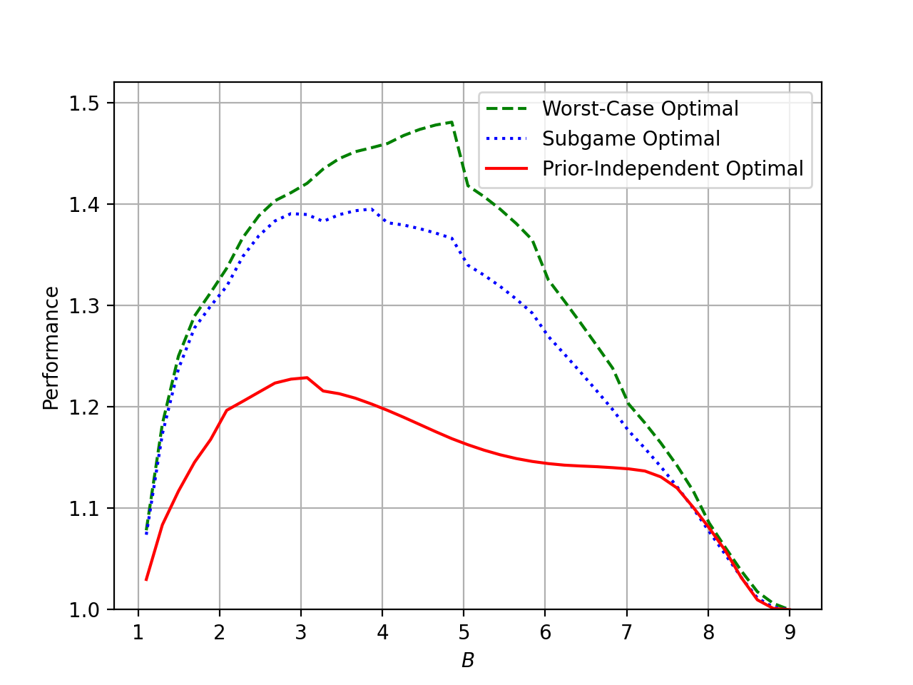
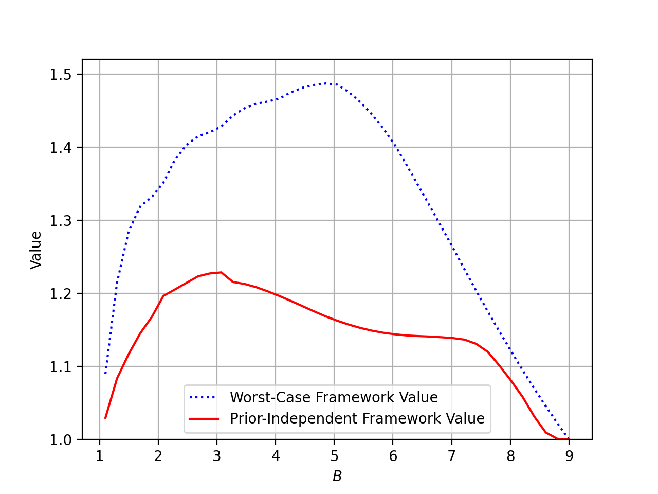
We empirically compare the algorithms in the prior-independent framework. Figure 1 plots the approximation ratio of each algorithm against the worst-case distribution over distributions. The subgame optimal algorithm outperforms the worst-case optimal algorithm. The near-optimal prior-independent algorithm has the best performance out of the three.

We compare the structural behavior of the algorithms. The optimal prior-independent algorithm exhibits more extreme choices than the worst-case and subgame optimal algorithms: it stops more aggressively after observing a good day, and less aggressively after observing a bad day.

Refer to caption — Figure 1: The time horizon is fixed at $T=9$ . The stopping cost $B$ is varied continuously over $[1,T]$ . The figure plots the approximation ratio of each algorithm against the worst-case distribution of the adversary in the prior-independent framework.

Together, these frameworks offer complementary approaches to robust algorithm design, giving practitioners principled options based on the reliability of their knowledge about the input distribution. When the input exhibits some distributional structure, it is natural to optimize for the prior-independent objective. In contrast, when no such structure can be assumed, one may instead aim for a subgame optimal algorithm.

1.2 Limitations Of Our Analysis

We note some of the assumptions and limitations of our analysis. First, the prior-independent framework assumes that input coordinates are drawn independently and identically. Although standard in the prior-independent literature, real-world inputs often exhibit correlation. Developing a meaningful intermediate model of correlation remains an important direction for capturing a more realistic setting. Second, our analysis does not yield an analytical characterization of the optimal prior-independent algorithm, even for a simple and canonical setting such as ski-rental. One way forward may be to identify simple approximations of the prior-independent optimal.

1.3 Related Work

A central theme in beyond worst-case analysis is the study of online algorithms with distributional information. Koutsoupias and Papadimitriou [22] introduce a diffuse adversary model, in which performance is measured by the worst-case ratio – taken over input distributions – between the algorithm’s expected cost and that of the optimal offline benchmark. In contrast to their setting, the benchmark in the prior-independent framework is the optimal online algorithm with full knowledge of the input distribution. Dehghani et al. [7] study the $k$ -server problem with distributional advice, in which each request is sampled from a known independent distribution specific to that period. They aim to design algorithms that approximate the Bayesian optimal benchmark, but the approach is not prior-independent since the algorithm depends on the request distribution. Mahdian et al. [24] study online algorithms in a stochastic setting and propose a general framework for resource allocation that combines two types of guarantees: one from an algorithm tailored to specific distributional assumptions and another from a classical worst-case algorithm, thereby achieving a best-of-both-worlds guarantee.

There is a substantial body of work in the Bayesian online selection literature that designs online policies competing against the Bayesian optimal benchmark. A canonical problem in this area considers a seller with multiple items facing buyers who arrive online and submit (typically random) bids; the seller must allocate items without knowledge of future arrivals. Some variations of this online auction and pricing problem include Huang et al. [19], Anari et al. [1], Papadimitriou et al. [25], Braverman et al. [5] and Fu et al. [12]. Algorithms in these papers generally assume knowledge of the input distribution, or, alternatively, provide constant-factor approximations to the Bayesian optimum. In a prior-independent setting, Babaioff et al. [3] achieve constant-factor guarantees. By contrast, our work identifies conditions under which an FPTAS exists, enabling a direct comparison between robust algorithms in the prior-independent and worst-case frameworks.

Two recent works establish prior-independent results in the context of online algorithm design. Hartline and Johnsen [15] develop a general method for proving lower bounds on the performance of prior-independent algorithms. Hartline et al. [16] link prior-independent design to worst-case benchmark problems and, in their application to no-regret expert learning, establish that the follow-the-leader algorithm is prior-independent optimal.

The ski-rental problem has also been studied from a distributional perspective. Madry and Panigrahi [23] analyze a two-stage game formulation of the problem under distributional assumptions. Diakonikolas et al. [8] study a setting closely related to ours, where the good days are drawn from a log-concave distribution. A key distinction, however, is that their algorithm relies on access to samples from the distribution. By contrast, our problem can be viewed as the sample-free analogue of their framework.

Beyond this, our notions of subgame optimality and prior-independence can be interpreted as providing robustness and consistency guarantees – two performance criteria that are central in the literature on online algorithms with advice (see Purohit et al. [26] and Gollapudi and Panigrahi [13]). In our setting, the “advice” available to the algorithm is the specification of a class of i.i.d. input distributions. While this connection is conceptually useful, we do not pursue the algorithms-with-advice perspective further in this paper.

Our analysis of prior-independent online algorithms can be interpreted as a reduction from computing a near-optimal prior-independent algorithm to computing an approximate Nash equilibrium in an infinite-dimensional two-player zero-sum game. Following Khachiyan [21], equilibria in zero-sum games can be computed in time polynomial in the size of the payoff matrix. A large body of work has since developed online-learning methods for approximating Nash equilibria. When both players adopt no-regret learning strategies (e.g., Freund and Schapire [10], their average play converges to a Nash equilibrium at a rate of $O(1/\sqrt{T})$ . Daskalakis et al. [6] present a no-regret learning algorithm that, when used by both players simultaneously, guarantees convergence to an approximate equilibrium at a faster rate of $O(\log T/T)$ , while retaining the $O(1/\sqrt{T})$ guarantee in adversarial environments. These algorithms, however, are not applicable in our setting since the space of algorithms is exponentially large. Assos et al. [2] study equilibrium computation in two-player zero-sum games with general payoffs and infinite action spaces assuming access to a best-response oracle. Their approximation bounds are exponential in the desired accuracy and thus not directly applicable in our setting.

2 Robust Algorithm Design

Let $T$ denote the input length of the online algorithm. The input space is $\mathcal{X}^{T}$ , and a particular input is denoted by $\textbf{X}=(X_{1},\dots,X_{T})$ , where each element $X_{i}\in\mathcal{X}$ . Let $\mathcal{F}\subseteq\Delta(\mathcal{X}^{T})$ denote the class of distributions over inputs, where a distribution is denoted by $F$ . The class of feasible deterministic algorithms is denoted by $\mathcal{A}$ , with a representative algorithm $A\in\mathcal{A}$ . The expected performance of $A$ under $F$ is

A(F)=\mathbf{E}_{\textbf{X}\sim F}[A(\textbf{X})].

A randomized algorithm $A^{\prime}\in\Delta(\mathcal{A})$ is a distribution over deterministic algorithms, with expected performance

A^{\prime}(F)=\mathbf{E}_{A\sim A^{\prime}}[A(F)].

We now turn to the Bayesian optimal framework and the robust algorithm design framework.

Definition 1.

The Bayesian optimal algorithm design problem is given by a distribution $F$ and a family of algorithms $\mathcal{A}$ and asks for the algorithm $\text{OPT}_{F}$ with the minimum expected cost

\text{OPT}_{F}(F)=\operatorname*{arg\,min}_{A\in\mathcal{A}}A(F).

It is without loss of generality to restrict the Bayesian optimal algorithm design problem to deterministic algorithms. For any randomized algorithm, one can identify a deterministic algorithm in its support that incurs weakly lower cost. We now turn to the definition of the robust algorithm design framework.

Definition 2.

The robust algorithm design problem is given by a family of distributions $\mathcal{F}$ , a family of algorithms $\mathcal{A}$ and solves the minimization problem

\beta=\min_{A^{\prime}\in\Delta(\mathcal{A})}\max_{F\in\mathcal{F}}\frac{A^{% \prime}(F)}{\text{OPT}_{F}(F)}.

The algorithm which solves it is denoted as $\text{OPT}_{\mathcal{F}}$ .

Solving this optimization problem guarantees a multiplicative approximation factor of $\beta$ relative to the Bayesian optimal performance for all distributions in the feasible class.

The robust algorithm design problem can be formulated as a two-player zero-sum game between an algorithm player, with strategy set $\mathcal{A}$ , and an adversary, with strategy set $\mathcal{F}$ . The optimization problem corresponds to computing a mixed min-max strategy profile in this game, which guarantees a $\beta$ -approximation to the Bayesian optimal performance.

Our focus will be on two special cases of the robust algorithm design problem: prior-independent algorithm design and worst-case algorithm design, each distinguished by different distributional assumptions over the input space.

Prior-Independent Algorithm Design

A distribution in $\mathcal{F}$ is such that, for $D\in\Delta(\mathcal{X})$ , $X_{i}\sim D$ , i.i.d. across all $i\in[T]$ , that is,

\mathcal{F}:=\{X_{i}\sim D,\text{ i.i.d. }\forall i\in[T]:D\in\Delta(\mathcal{% X})\}.

Worst-Case Algorithm Design

The class of distributions is degenerate distributions over the input space, that is,

\mathcal{F}:=\{\text{Pr}[\mathbf{X}]=1:\mathbf{X}\in\mathcal{X}^{T}\}.

We formalize the above ideas using the finite-horizon ski-rental problem, which serves as our primary application of beyond worst-case analysis in this paper.

2.1 Finite-Horizon Ski-Rental Problem

An agent observes an online sequence of days, each having either good or bad weather. The agent has knowledge about the length of the sequence, denoted by $T$ , but observes the weather of each day in an online fashion. We represent the sequence as $\textbf{X}\in\{0,1\}^{T}$ where the $i^{th}$ component of X, represented by $X_{i}$ , is the weather on the $i^{th}$ day. A good weather day corresponds to $X_{i}=1$ while a bad weather day corresponds to $X_{i}=0$ . Upon observing the weather, the agent needs to decide whether to stop, incurring a fixed known cost $B\in\mathbb{R}^{+}$ , or continue, incurring a normalized cost of $1$ on good days and $0$ on bad days. This decision must be made without knowledge of the future sequence. Once the agent decides to stop, no further costs are incurred.

A deterministic algorithm is specified as a tuple of functions mapping observed sequences of days to the actions stop or continue.

Definition 3.

A deterministic algorithm is a tuple of functions $(A_{1},A_{2},\dots,A_{T})$ where

A_{i}:\left(X_{1},\dots,X_{i}\right)\to\{S,C\}\quad\forall\left(X_{1},\dots,X_% {i}\right)\in\{0,1\}^{i}\quad\forall i\in[T]

where $S$ is a decision to stop and $C$ is a decision to continue.

Prior-Independent Algorithm Design

Each day the weather is good with some probability $p$ , i.i.d. over $T$ days. The class of distributions is $\mathcal{P}=[\delta,1]$ , with $\delta>0$ . ⁴⁴4We consider the range of feasible distributions to be $[\delta,1]$ , for $\delta>0$ as $p=0$ is a null instance for which the Bayesian optimal performance is zero. This would lead to an undefined payoff in the prior-independent framework. We do not make any assumptions on the magnitude of $\delta$ . It can be arbitrarily small, but must be positive. An optimal prior-independent algorithm solves

\min_{A^{\prime}\in\Delta(\mathcal{A})}\left[\max_{p\in[\delta,1]}\frac{% \mathbf{E}_{A\sim A^{\prime}}[A(p)]}{\text{OPT}_{p}(p)}\right].

Worst-Case Algorithm Design

An optimal worst-case algorithm is given by

\min_{A^{\prime}\in\Delta(\mathcal{A})}\max_{\textbf{X}\in\{0,1\}^{T}}\frac{% \mathbf{E}_{A\sim A^{\prime}}[A(\textbf{X})]}{\text{OPT}_{\textbf{X}}(\textbf{% X})},

where $\text{OPT}_{\textbf{X}}(\textbf{X})$ denotes the optimal hindsight cost for the sequence X. If a sequence contains $k=\sum_{i=1}^{T}X_{i}$ good weather days, then $\text{OPT}_{\textbf{X}}(\textbf{X})=\min\{k,B\}$ .

To solve the robust algorithm design problem, we draw on standard equilibrium concepts from game theory. For completeness, we review these preliminaries in the full version of the paper.

3 Efficient Computation Of Robust Algorithms

This section adopts a computational perspective on robust algorithm design. Although a full analytical characterization is generally intractable, a game-theoretic formulation offers a tractable pathway for computing optimal algorithms.

In particular, the problem reduces to computing a mixed Nash equilibrium in the zero-sum game between algorithm and adversary. The difficulty lies in the fact that the algorithm’s pure strategy space is exponentially large, while the adversary has infinitely many pure strategies. As a result, traditional methods for equilibrium computation – such as no-regret learning (Freund and Schapire [11]) or the Ellipsoid algorithm (Khachiyan [21]) – cannot be applied directly.

We identify structural properties that reduce the problem to a half-infinite action game in which one player has access to a best response oracle. This oracle computes a best response to any mixed strategy of the opposing player in time polynomial in the size of the support of that strategy. In such settings, equilibrium computation is known to be efficient.

Lemma 4 (Freund and Schapire [10] and Hellerstein et al. [18]).

There exists an algorithm which computes an $\epsilon$ -approximate Nash equilibrium in a two-player zero-sum game, where one player has a finite set of actions and the other player has access to a best response oracle, in time which is polynomial in the number of actions of the first player, $1/{\epsilon}$ and the upper bound on the payoffs of the game.

We now state the properties required by our framework.

Property 1 (Small-Cover).

Given $\epsilon>0$ , there exists a set $\mathcal{F}_{\epsilon}$ of size $\operatorname{poly}\left(T,\frac{1}{\epsilon}\right)$ , where $T$ is the size of the input, such that for every $F\in\mathcal{F}$ , there exists a corresponding $F_{\epsilon}\in\mathcal{F}_{\epsilon}$ , such that

\left|\frac{A(F)}{\text{OPT}_{F}(F)}-\frac{A(F_{\epsilon})}{\text{OPT}_{F_{% \epsilon}}(F_{\epsilon})}\right|\leq\frac{\epsilon}{4},

for all algorithms $A\in\mathcal{A}$ .

Property 2 (Efficient Best Response).

There exists an algorithm which solves the optimization problem

A_{F^{\prime}}=\operatorname*{arg\,min}_{A\in\mathcal{A}}\mathbf{E}_{F\sim F^{% \prime}}\left[\frac{A(F)}{\text{OPT}_{F}(F)}\right]

for any $F^{\prime}\in\Delta(\mathcal{F}_{\epsilon})$ , efficiently in the size of the representation of $F^{\prime}$ and length of the input $T$ .

Property 3 (Efficient Utility Computation).

For any $F^{\prime}\in\Delta(\mathcal{F}_{\epsilon})$ , for the optimal algorithm $A_{F^{\prime}}$ obtained by 2, there exists an algorithm which computes, for any $F\in\mathcal{F}_{\epsilon}$ , the utility $\frac{A_{F^{\prime}}(F)}{\text{OPT}_{F}(F)}$ in run-time $\text{poly}(T)$ .

Property 4 (Bounded Best Response Utility).

For any $F^{\prime}\in\Delta(\mathcal{F}_{\epsilon})$ , any best response $A_{F^{\prime}}$ is such that, for any $F\in\mathcal{F}_{\epsilon}$ , the utility $\frac{A_{F^{\prime}}(F)}{\text{OPT}_{F}(F)}$ is at most $\text{poly}(T)$ .

Remarks on the sufficient conditions

Any problem instance that admits an efficient dynamic program satisfies Efficient Best Response. Moreover, the existence of such a dynamic program typically ensures that Efficient Utility Computation and Bounded Best Response Utility hold. Although the property formally requires computing an optimal algorithm, an approximately optimal algorithm is sufficient; in this case, performance degrades linearly with the approximation error in the best response.

Small-Cover intuitively says that the class of distributions $\mathcal{F}$ can be approximated by a finite subclass $\mathcal{F}_{\epsilon}$ . This property depends on the specific distributions and algorithms under consideration. Although it may appear to be a strong requirement – since it must hold for all $A\in\mathcal{A}$ – in practice the algorithm class can often be restricted to a subclass with the property that, for any distribution chosen by the adversary, an optimal best response of the algorithm lies within it. The four properties can then be applied to this restricted subclass.

Further concerning Small-Cover, it is relatively straightforward to show that a fixed algorithm performs similarly on two nearby distributions. The difficulty lies in bounding the ratio of the algorithm’s performance to that of the Bayesian optimal. Since the Bayesian optimal cost can be arbitrarily small, naive bounds on this ratio can become very loose, necessitating an excessively fine cover and leading to longer running times. In Section 3.1, we establish a non-trivial bound on this objective, despite the possibility of vanishing Bayesian optimal costs.

The primary application in this paper is the finite-horizon ski-rental problem. Beyond this setting, the properties we develop have proved useful in other areas of algorithm design. For instance, Guo et al. [14] build on our framework to compute a near-optimal prior-independent information aggregator, overcoming the key technical challenge of constructing a small cover of the space of information structures. We now state our main result.

Theorem 5.

If the class of algorithms $\mathcal{A}$ and the class of distributions $\mathcal{F}$ satisfy Small-Cover, Efficient Best Response, Efficient Utility Computation and Bounded Best Response Utility, an approximate robust optimal algorithm can be computed in time $\operatorname{poly}\left(T,\frac{1}{\epsilon}\right)$ for inputs of length $T$ .

We now turn to the proof of Theorem 5. A challenge in computing an optimal algorithm is the size of the players’ strategy spaces. A natural direction leads to the question of computing a near-optimal robust algorithm which reduces to computing an approximate Nash equilibrium. The key idea is to adopt the adversary’s perspective and learn a worst-case distribution over inputs. The four properties then ensure the existence of a reduced strategy game in which any approximate equilibrium also serves as an approximate equilibrium of the original game.

Original Game:: Pure strategy set of the algorithm player is $\mathcal{A}$ . Pure strategy set of the adversary is $\mathcal{F}$ .
Reduced Game:: Pure strategy set of the algorithm player is $\mathcal{A}$ . Pure strategy set of the adversary is $\mathcal{F}_{\epsilon}$ .

We begin by establishing two facts that relate equilibria in the original and reduced games. For any algorithm and any adversary strategy in the original game, one can identify a corresponding adversary strategy in the reduced game whose payoff is $\epsilon$ -close.

Lemma 6.

Assuming Small-Cover, for a fixed algorithm strategy, for every adversary strategy in the original game, there exists an adversary strategy in the reduced game such that their payoffs are $\frac{\epsilon}{4}$ -close to each other.

Utilizing Lemma 6, we next establish that approximate equilibria in the reduced game transfer to the original game.

Lemma 7.

Assuming Small-Cover, an $\frac{\epsilon}{4}$ -approximate Nash equilibrium in the reduced game is an $\frac{\epsilon}{2}$ -approximate Nash equilibrium in the original game.

An application of Lemma 4 to the reduced game implies the existence of a FPTAS to compute an optimal robust algorithm. The learning algorithm takes the point of view of the adversary by learning a worst-case distribution over inputs. A complete proof is provided below.

Proof of Theorem 5.

Applying the algorithm in Lemma 4, we compute an $\frac{\epsilon}{4}$ -approximate Nash equilibrium. By Efficient Best Response, Efficient Utility Computation, Bounded Best Response Utility and Small-Cover, the run-time of the algorithm in Lemma 4 to compute an $\frac{\epsilon}{4}$ -approximate Nash equilibrium will be $\text{poly}\left(T,\frac{1}{\epsilon}\right)$ . By Lemma 7, an $\frac{\epsilon}{4}$ -approximate Nash equilibrium in the reduced game will be an $\frac{\epsilon}{2}$ -approximate Nash equilibrium in the original game. It follows that the mixed strategy of the algorithm player will be an $\epsilon$ -approximate prior-independent optimal algorithm. $\hfill\blacktriangleleft$

Before applying the framework to the ski-rental problem, we establish a preliminary result that restricts the class of algorithms to be considered when computing a robust algorithm. Specifically, it suffices to reduce the algorithm player’s strategy space to best-response algorithms.

Lemma 8.

In a two-player game between player $1$ , with pure strategy set $\mathcal{A}$ , and player $2$ , with pure strategy set $\mathcal{F}$ , if for any mixed strategy that player $2$ chooses, a best response of player $1$ lies in a subset of strategies $\mathcal{A}^{*}\subset\mathcal{A}$ , then an $\epsilon$ -approximate Nash equilibrium in the reduced game between player $1$ and player $2$ with pure strategy sets $\mathcal{A}^{*}$ and $\mathcal{F}$ respectively is an $\epsilon$ -approximate Nash equilibrium in the original game.

3.1 Prior-Independent Finite-Horizon Ski-Rental Problem

This section establishes that the prior-independent ski-rental problem satisfies the Small-Cover, Efficient Best Response, Efficient Utility Computation and Bounded Best Response Utility properties. By Theorem 5, it follows that there exists an FPTAS for computing a near-optimal prior-independent algorithm.

Definition 9.

The prior-independent problem is given by the class of distributions $\mathcal{P}=[\delta,1]$ , for $\delta>0$ , the class of algorithms $\mathcal{A}$ and solves for the randomized algorithm that optimizes for the worst-case ratio

\beta=\min_{A^{\prime}\in\Delta(\mathcal{A})}\left[\max_{p\in[\delta,1]}\frac{% \mathbf{E}_{A\sim A^{\prime}}[A(p)]}{\text{OPT}_{p}(p)}\right]

In general, the prior-independent ratio will depend on the stopping cost $B$ and time horizon $T$ . For illustration, Figure 2 plots the prior-independent ratio of the ski-rental problem for various instances of $B$ and $T$ . The approximation parameter is set to $\epsilon=0.01$ , and the underlying zero-sum game is approximately solved using an online learning reduction with the Multiplicative Weights Update algorithm (Freund and Schapire [11]). ⁵⁵5We state the run-time guarantee of the Multiplicative Weights Algorithm in Freund and Schapire [11] as established in. Consider a two-player zero-sum game in which the first-player has a strategy space of size $d$ , the second player has access to a best-response oracle with run-time $\mathcal{L}$ , and payoffs are uniformly bounded by $\bar{u}$ . Then an $\epsilon$ -approximate equilibrium can be computed via Multiplicative Weights in time $O\left(\frac{\bar{u}^{2}\mathcal{L}\log d}{\epsilon^{2}}\right)$ .

The plots show that the prior-independent ratios achieved are strictly better than the corresponding worst-case ratios. A structural comparison between optimal algorithms under the two frameworks is provided in Section 5.

3.1.1 Characterization of the Bayesian Optimal Algorithm

We begin by characterizing the Bayesian optimal algorithm for a given horizon $T$ , stop cost $B\in(1,T)$ , ⁶⁶6The prior-independent problem is trivial when $B\geq T$ . This is because no matter what the distribution $p$ is, the Bayesian optimal is to always continue and thus the agent strategy of continuing for all days achieves the best possible prior-independent ratio of one. From now on we only consider $B<T$ . and distribution $p\in[\delta,1]$ . This characterization admits a closed-form expression for the Bayesian optimal cost $\text{OPT}_{p}(p)$ .

Theorem 10.

For a given time horizon $T$ and stop cost $B$ , the Bayesian optimal algorithm, for a distribution $p\in\left[\frac{B-1}{T-1},1\right]$ , is to stop on a good day at time index $k$ if $p\geq\frac{B-1}{T-k}$ , otherwise continue, where $k\in[\min\{\left\lceil T-B\right\rceil,T-1\}]$ . For $p\in[\delta,\frac{B-1}{T-1}]$ , the Bayesian optimal algorithm always continues.

For $p\in\left[\frac{B-1}{T-1},1\right]$ , let $k$ denote the last day on which algorithm $\text{OPT}_{p}$ stops. The Bayesian optimal cost is then

\text{OPT}_{p}(p)=B[1-(1-p)^{k}]+(1-p)^{k}p(T-k).

When $p\in\left[\delta,\frac{B-1}{T-1}\right]$ , since the algorithm always continues, the cost is simply

\text{OPT}_{p}(p)=Tp.

Analyzing the expected cost of a general algorithm $A$ will be important both for understanding utility behavior in the associated game and for establishing the Small-Cover property.

3.1.2 Properties of the Prior-Independent Ski-Rental Problem

In this section, we verify that the properties required by the framework are satisfied. To this end, we establish that it is without loss of generality to restrict attention to algorithms that are information-symmetric and that never stop on a bad-weather day.

Backwards Induction is an algorithm that, for any randomization over distributions $P$ , solves the optimization problem

\min_{A\in\mathcal{A}}\mathbf{E}_{p\sim P}\left[\frac{A(p)}{\text{OPT}_{p}(p)}% \right].

It is useful to note that for any distribution over distributions, a best response never stops on a bad-weather day. Indeed, any strategy that does so is strictly dominated by one that instead waits to stop at the next good day. Hence, it is without loss of generality to restrict attention to such algorithms.

Moreover, an optimal algorithm bases its decisions on the number of good days observed in a given prefix of the sequence. We refer to such strategies as information-symmetric. Formally, in Definition 11, the first argument of $A_{i}$ represents the number of good weather days observed in the first $(i-1)$ days, while the second argument specifies the weather on the $i^{\text{th}}$ day.

Definition 11.

An information-symmetric deterministic algorithm $A=(A_{1},A_{2},\dots,A_{T})$ is such that

A_{i}:\{0,1,\dots,i-1\}\times\{0,1\}\to\{S,C\}\quad\forall\quad i\in[T]

where $S$ is a decision to stop and $C$ is a decision to continue.

We show that for any fixed distribution that the adversary plays, an optimal algorithm obtained by backwards induction is information-symmetric.

Lemma 12.

For any distribution over distributions, $P\in\Delta([\delta,1])$ , that the adversary plays, an optimal algorithm for that distribution obtained by Backwards Induction is information-symmetric.

A direct application of Lemma 8 and Lemma 12 shows that it is without loss of generality to restrict attention to algorithms that are information-symmetric and never stop on a bad weather day:

\mathcal{A}=\{A:A\quad\text{is information-symmetric; does not stop on % observing bad weather}\}.

From this point onward, we restrict attention to algorithms from the class defined above. Under this restriction to information-symmetric algorithms, we can show that, for any discrete distribution chosen by the adversary, an optimal algorithm can be computed efficiently via Backwards Induction, thereby satisfying the Efficient Best Response property.

Theorem 13.

For a discrete distribution with support size $|\operatorname{supp}(P)|$ , Backwards Induction finds an optimal solution to the optimization problem

\min_{A\in\mathcal{A}}\mathbf{E}_{p\sim P}\left[\frac{A(p)}{\text{OPT}_{p}(p)}% \right],

in time $O(|\operatorname{supp}(P)|T^{3})$ .

A similar argument establishes the Efficient Utility Computation property as well.

Lemma 14.

For any information-symmetric algorithm $A$ , and any $p\in[\delta,1]$ , the utility $u(A,p)=\frac{A(p)}{\text{OPT}_{p}(p)}$ can be computed in time $\operatorname{poly}(T)$ .

We now show that the Small-Cover property is satisfied. Specifically, we construct an $\epsilon$ -cover of the probability space that preserves the Lipschitz property in utility space. Recall that the utility is expressed as a ratio, with a denominator that can become arbitrarily small. To ensure utilities remain close, we discretize the interval $[\delta,1]$ into a suitable grid. The intuition is that the expected performance of an algorithm changes only slightly when evaluated at two probabilities that are close to each other, making such a discretization sufficient.

Lemma 15.

For a fixed algorithm $A$ , for any two probabilities $p_{\alpha},p_{\beta}$ such that

|p_{\alpha}-p_{\beta}|\leq\frac{\epsilon}{T^{2}},

the expected costs of the algorithm are such that

|A(p_{\alpha})-A(p_{\beta})|\leq\frac{\epsilon(B+T)}{T}.

While the result above establishes a notion of performance closeness, our main interest lies in utility closeness: for probabilities that are close, the utility $A(p)/\text{OPT}_{p}(p)$ should also be close for any algorithm. A trivial lower bound of $T\delta$ on the Bayesian optimal cost yields a bound that depends on $1/\delta$ , which is undesirable since $\delta$ may be arbitrarily small. We instead establish a tighter utility-closeness bound that is independent of $\delta$ . Proving that the ratio of utilities remains close requires an additional decomposition property of the algorithmic cost.

Lemma 16.

For any $k\in[\min\{\left\lceil T-B\right\rceil,T-1\}]$ , consider two probabilities $p_{\alpha},p_{\beta}$ in the interval $\left(\frac{B-1}{T-k},\min\left\{\frac{B-1}{T-k-1},1\right\}\right]$ such that

|p_{\alpha}-p_{\beta}|\leq\frac{\epsilon}{8(B+1)^{2}(T+1)^{2}T}.

Then for any algorithm $A$ , we have

|u(A,p_{\alpha})-u(A,p_{\beta})|\leq\frac{\epsilon}{4}.

This utility-closeness property also holds when $p_{\alpha},p_{\beta}$ are in the interval $\left[\delta,\frac{B-1}{T-1}\right]$ .

Our focus has been on establishing the Small-Cover property, during which we also show the Bounded Best Response Utility property.

A key point is that the discretization must be performed separately within each interval where the Bayesian optimal algorithm remains unchanged. As formalized in Lemma 16, the utility of an algorithm is close only for probabilities lying in the same such interval. When two nearby probabilities fall into different intervals, the Lipshitz bound no longer applies.

Theorem 17.

The class of algorithms $\mathcal{A}$ and the class of distributions $\mathcal{P}$ in the prior-independent ski-rental problem satisfy Small-Cover.

Having shown that all four properties in the framework are satisfied, we give a bound on the running time to compute an approximate-optimal prior-independent ski-rental algorithm.

Theorem 18.

There exists an algorithm to find an $\epsilon$ -approximate prior-independent optimal algorithm in time $\tilde{O}(T^{12}\epsilon^{-3})$ .

Remarks on the computational perspective

An alternative approach is to learn the distribution $p$ . This would involve continuing on an initial set of days to form an empirical estimate of the probability. We do not pursue this direction for the following reason: such algorithms typically approximate the Bayesian optimal, with the approximation factor improving as $T$ grows. Our focus is on (near) optimality, as it distills and allows a clear comparison of features of each framework. Moreover, our simulations (see Section 5) reveal that optimal prior-independent algorithms are structurally aggressive on moderate input lengths, tending to buy as soon as a good day is observed rather than delaying to collect data for estimation.

Finally, we note that our computational framework is not tied to the online nature of the problem; it applies more broadly to any robust environment that admits a suitable discretization.

4 Subgame Optimal Algorithms

This section examines the worst-case paradigm of online algorithm design and introduces the notion of subgame optimal algorithms. These algorithms are worst-case optimal but can also exploit mistakes made by the adversary. In Section 4.1, we formally define subgame optimality and contrast it with standard worst-case optimality. In Section 4.2, we apply these ideas to the finite-horizon ski-rental problem.

4.1 Strategic Form and Extensive Form Representation

The worst-case algorithm design paradigm solves

\beta=\min_{A^{\prime}\in\Delta(\mathcal{A})}\max_{\mathbf{X}}\frac{A^{\prime}% (\mathbf{X})}{\text{OPT}_{\mathbf{X}}(\mathbf{X})},

where $\text{OPT}_{\mathbf{X}}(\mathbf{X})$ denotes the cost of the optimal offline algorithm with full knowledge of the sequence $\mathbf{X}$ .

As noted earlier, this problem reduces to solving for a mixed Nash equilibrium in a zero-sum game between the algorithm player, whose strategy set consists of algorithms, and the adversary, whose strategy set consists of input sequences. Our analysis focuses on a non-adaptive adversary, one that commits to an input sequence in advance without observing the algorithm’s decisions.

A worst-case algorithm can be found by solving for equilibrium in the strategic form representation of the game. In this framework, the adversary selects a worst-case input sequence, referred to as on-path; any input on which the algorithm performs strictly better is off-path. A consequence of the framework’s assumptions is that the resulting algorithm need not perform optimally off-path and may fail to exploit adversarial mistakes. This motivates the consideration of stronger equilibrium concepts.

A natural representation of an online problem is through its extensive form representation (see Chapter 6 in the textbook by Borodin and El-Yaniv [4] for an introduction to the different representations of a game). An algorithm obtained through the strategic form game need not take optimal decisions at each decision node in the extensive form game. A subgame optimal strategy captures the notion of off-path optimality. Such a strategy takes an optimal decision at every node in the decision tree.

It is useful to clarify what we mean by a subgame in the setting of an oblivious adversary. By definition, an oblivious adversary commits to an input sequence in advance, without observing the algorithm’s decisions as they unfold. The sequence is then revealed incrementally to the algorithm over time. In game-theoretic terms, all decision nodes of the adversary lie in the same information set.

A subgame in our setting is defined with respect to each partially revealed input sequence $\mathbf{X}\in\{0,1\}^{t-1}$ , for every time index $t\in[T]$ . Conditioned on continuing for $(t-1)$ days, the subgame reduces to a finite-horizon ski-rental problem with horizon $T-t+1$ , played against an oblivious adversary and with utilities specified as follows. The algorithm’s cost consists of the rental cost incurred during the initial $(t-1)$ days of continuation, while the benchmark hindsight cost is evaluated with respect to the full input sequence $\mathbf{X}$ .

Definition 19 (Subgame Optimal Algorithm).

Consider an online algorithm design problem and its extensive form representation. An algorithm is said to be subgame optimal if it is optimal in every subgame. Such an algorithm is denoted by SG-OPT.

With this notion, we can define a new benchmark for the algorithm design problem.

Definition 20 (Subgame Optimal Benchmark).

The performance of an algorithm $A$ , against the subgame optimal benchmark is

\max_{\mathbf{X}}\frac{A(\mathbf{X})}{\text{SG-OPT}(\mathbf{X})}.

In general, solving for a subgame optimal algorithm may be computationally and analytically intractable. The benchmark allows for a comparison across different worst-case algorithms, with the approximation ratio capturing their performance on off-path inputs.

4.2 Finite-Horizon Ski-Rental Problem

This section applies the concept of subgame optimality and compares its performance to an optimal worst-case algorithm.

4.2.1 Optimal Randomized Algorithm

We begin by solving for an optimal randomized algorithm, thereby determining the competitive ratio of the finite-horizon ski-rental problem. As noted earlier, this algorithm can be obtained by solving for equilibrium in the strategic-form representation of the game, denoted by SRP.

We show that it is without loss of generality to restrict the adversary to providing a contiguous block of good weather days followed by bad weather days. To formalize this simplification, we define a reduced two-player zero-sum game, denoted by SRP-R.

In SRP-R, the adversary’s pure strategies are indexed by the number of initial good days. Formally,

\mathcal{F}_{g}:=\{F^{k}:k\in\{1,2,\dots,T\}\},

where $F^{k}$ denotes the input with $k$ consecutive good days followed by bad days. The algorithm’s pure strategies are indexed by the number of good weather days for which they continue after which they stop. Formally,

\mathcal{A}_{g}:=\{A^{l}:l\in\{0,1,\dots,T\}\},

where $A^{l}$ denotes the algorithm which continues for the first $l$ good days after which it stops on the $(l+1)^{\text{st}}$ good weather day. A deterministic algorithm in $\mathcal{A}_{g}$ implicitly defines the decision it takes on all possible input sequences; the algorithm ignores any bad day by continuing, only keeping a track of the number of good days. The pure strategy $A_{T}$ continues for all days.

The utility to the adversary player for algorithm strategy $A^{l}$ and adversary strategy $F^{k}$ is

u(A^{l},F^{k})=\left\{\begin{array}[]{ll}\frac{l+B}{\min\{k,B\}}&\mbox{if }k>l% \\ \frac{k}{\min\{k,B\}}&\mbox{if }k\leq l\end{array}\right..

We establish that any mixed Nash equilibrium in SRP-R is also a mixed Nash equilibrium in SRP. Consequently, the algorithm player’s mixed strategy in SRP-R constitutes an optimal worst-case algorithm.

Lemma 21.

Any mixed Nash equilibrium in SRP-R is a mixed Nash equilibrium in SRP.

A sketch of the proof is as follows. Given a mixed-equilibrium in SRP-R, we must verify that no player has an incentive to deviate in SRP. For the algorithm player, this is immediate, as its strategy remains optimal. For the adversary, the off-path actions of deterministic algorithms in $\mathcal{A}_{g}$ ensure that deviations yield no improvement.

We now solve for an equilibrium in SRP-R. The strategy space of each player can be further reduced as follows. The set of pure strategies $\{F^{k}:k\in\{\left\lceil B\right\rceil,\dots,T-1\}\}$ is weakly dominated by $F_{T}$ . To see this, note that the optimal hindsight cost for any strategy $F^{k}$ where $k\in\{\left\lceil B\right\rceil,\dots,T\}\}$ is $B$ . Among these, $F^{T}$ yields a weakly higher cost for every algorithm strategy by providing more good-weather days. For the algorithm player, the set of pure strategies $\{A^{l}:l\in\{T-\left\lfloor B\right\rfloor,\dots,T-1\}\}$ is weakly dominated by $A^{T}$ . The algorithm will never choose to stop within the last $\left\lfloor B\right\rfloor$ time steps for any input sequence, since it incurs a smaller cost by continuing.

Thus, in solving for an equilibrium in SRP-R, it is without loss to restrict attention to the zero-sum game where the algorithm’s strategy set is

\mathcal{A}^{\prime}_{g}=\{A^{l}:l\in\{0,\dots,T-\left\lfloor B\right\rfloor-1% \}\cup\{T\}\},

and the adversary’s strategy set is

\mathcal{F}^{\prime}_{g}=\{F^{k}:k\in\{1,\dots,\left\lceil B\right\rceil-1\}% \cup\{T\}\}.

Theorem 22 characterizes the algorithm player’s strategy in a mixed Nash equilibrium of SRP-R. A sketch of the computation is as follows. A property of game theory is that in any mixed equilibria, the expected payoff of any pure strategy that has positive probability is the same (this payoff may differ across players). Depending on the value of $T$ relative to $B$ , we eliminate a set of strategies that are dominated in both $\mathcal{A}_{g}^{\prime}$ and $\mathcal{F}_{g}^{\prime}$ . The result follows by solving the system of equations obtained by equating the expected payoffs of strategies for each player in the resulting game.

Theorem 22.

A mixed strategy for the algorithm player in SRP-R:

$\blacksquare$

If $\left\lceil B\right\rceil+\left\lfloor B\right\rfloor\geq T+1$ , is,

$\text{Pr}^{T}[A^{l}]=\left(\frac{B}{B-1}\right)^{l}\times Pr[A^{0}]\quad% \forall l\in\{0,1,\dots,T-\left\lfloor B\right\rfloor-1\}$

$\text{Pr}^{T}[A^{T}]=\left(\frac{B}{T-B}\right)\left(\frac{B}{B-1}\right)^{T-% \left\lfloor B\right\rfloor-1}\left(B+\left\lfloor B\right\rfloor-T\right)% \times Pr[A^{0}].$
$\blacksquare$

If $\left\lceil B\right\rceil+\left\lfloor B\right\rfloor<T+1$ , is the same as the infinite-horizon ski-rental problem.

The worst-case competitive ratio is given by the value of SRP. This value is obtained by evaluating the expected utility of the adversary when the algorithm plays the mixed strategy described in Theorem 22. At equilibrium, the adversary is indifferent among all pure strategies in its support, so the expected utility coincides with the utility on the input sequence consisting of one good weather day followed by bad weather days.

If $\left\lceil B\right\rceil+\left\lfloor B\right\rfloor\geq T+1$ , the competitive ratio of the finite horizon ski-rental problem is

B\text{Pr}[A^{0}]+\sum_{l=1}^{T-\left\lfloor B\right\rfloor-1}\text{Pr}[A^{l}]% +\text{Pr}[A^{T}]=\frac{1}{1-\frac{(T-B)(B-1)}{B\left\lfloor B\right\rfloor% \left(\frac{B}{B-1}\right)^{T-\left\lfloor B\right\rfloor-1}}}.

If $\left\lceil B\right\rceil+\left\lfloor B\right\rfloor<T+1$ , the competitive ratio is

B\text{Pr}[A^{0}]+\sum_{l=1}^{\left\lceil B\right\rceil-1}\text{Pr}[A^{l}]=% \frac{1}{1-\frac{(\left\lceil B\right\rceil-1)}{B}\left(\frac{B-1}{B}\right)^{% \left\lceil B\right\rceil-1}}.

The ratios derived above can be compared to the competitive ratio of the classical ski-rental problem. Recall that in the classical setting the buy cost $B$ is a fixed integer and $T\rightarrow\infty$ . In this case, the ratio simplifies to

\frac{1}{1-\left(1-\frac{1}{B}\right)^{B}}

which recovers the classical result.

The randomized algorithm obtained in Theorem 22 is an optimal worst-case algorithm. However, it performs sub-optimally if the adversary does not provide the worst-case input sequence. In the next section, we solve for a subgame optimal algorithm. We show that the problem of characterizing a subgame optimal algorithm reduces to that of the optimal worst-case algorithm.

4.2.2 Subgame Optimal Algorithm

Consider an instance of the finite-horizon ski-rental problem with time horizon $T$ . It will be helpful to write the worst-case algorithm as a probability of stopping, conditional on observing and continuing on a sequence of contiguous good days. On observing $k$ contiguous good weather days, let $\eta_{k}^{T}$ denote the probability of stopping, conditional on continuing for these days. An immediate application of Theorem 22 gives us the following probabilities.

Corollary 23.

Consider an instance of the finite-horizon ski-rental problem with time horizon $T$ . Conditional on continuing for the first $(k-1)$ contiguous good weather days, the probability of stopping on the $k^{th}$ contiguous good weather day for an optimal randomized algorithm:

$\blacksquare$

If $\left\lceil B\right\rceil+\left\lfloor B\right\rfloor\geq T+1$ , for $k\in\{1,\dots,T-\left\lfloor B\right\rfloor\}$ , $\eta_{k}^{T}$ , is,

$\eta^{T}_{k}=\frac{1}{\frac{B\left\lfloor B\right\rfloor}{T-B}\left(\frac{B}{B% -1}\right)^{T-\left\lfloor B\right\rfloor-k}-(B-1)}.$
$\blacksquare$

If $\left\lceil B\right\rceil+\left\lfloor B\right\rfloor<T+1$ , for $k\in\{1,\dots,\left\lceil B\right\rceil-1\}$ ,

$\eta^{T}_{k}=\frac{1}{\left(B-1\right)\left(\frac{B}{B-1}\right)^{\left\lceil B% \right\rceil-k}\frac{B}{\left\lceil B\right\rceil-1}-(B-1)}.$

Additionally, $\eta^{T}_{\left\lceil B\right\rceil}=1$ .

To obtain a characterization for a subgame optimal algorithm, an optimal choice must be made at each decision node. Let us first observe the optimal strategy of the algorithm player on observing an initial contiguous sequence of bad weather days.

Lemma 24.

If the adversary initially provides a contiguous sequence of $l$ bad weather days, the optimal strategy of the algorithm player implements the optimal randomized algorithm for time horizon $(T-l)$ .

By Lemma 24, the probability of stopping on the sequence

\left(\underbrace{0,\dots,0,}_{l}\underbrace{1,\dots,1}_{k}\right),

conditional on continuing to time index $l+k-1$ , for the subgame optimal algorithm, is $\eta^{T-l}_{k}$ .

It remains to characterize the subgame optimal decisions on input sequences that start with a good weather day. We show that the conditional probability of stopping is the same as that of stopping had all the bad weather days been provided contiguously before providing the good weather days.

Lemma 25.

Consider a sub-sequence $(X_{1},\dots,X_{i},1)$ such that the total number of good weather days in $(X_{1},\dots,X_{i})$ is $k-1$ . The probability of stopping at $(X_{1},\dots,X_{i},1)$ , conditional on continuing up until this point, is $\eta_{k}^{T-i+k-1}$ .

This completes the reduction from subgame optimal algorithms to worst-case optimal algorithms. We can compare the worst-case algorithm in Theorem 22 to the subgame optimal algorithm. The objective we use is the worst-case ratio of their performances. Let WC-OPT denote a worst-case optimal algorithm and SG-OPT denote a subgame optimal algorithm. The competitive ratio according to the benchmark defined in Definition 20 is then

\max_{\mathbf{X}}\frac{\text{WC-OPT}(\mathbf{X})}{\text{SG-OPT}(\mathbf{X})}.

Theorem 26.

The competitive ratio against the subgame optimal benchmark for WC-OPT is the value of the game.

The result above tells us that the difference in the performance of worst-case optimal and subgame optimal can be as bad as the worst-case approximation ratio. If one expects to not see worst-case inputs, as has been argued for real-world applications Roughgarden [27], a subgame optimal algorithm gives better guarantees while maintaining the same worst-case approximation ratio.

5 Empirical Comparison of Frameworks

This section presents simulations evaluating the performance of the three robust algorithms: prior-independent optimal, subgame optimal and worst-case optimal. We begin by empirically comparing their performance within the prior-independent framework, and then examine the structural differences across the three algorithms.

5.1 Comparison of Algorithmic Performance

Our simulation setting is as follows. We fix the time horizon at $T=9$ and vary the stopping cost $B$ continuously over the interval $[1.1,T]$ . Figure 3 compares the algorithms in the prior-independent framework by plotting their approximation ratio against the worst-case adversary distribution for the near-optimal prior-independent algorithm.

Recall that in the prior-independent setting, the adversary chooses a distribution over probabilities. The plot illustrates the advantage a subgame optimal algorithm has over a worst-case algorithm. Because of the statistical assumptions in the prior-independent framework, every input sequence occurs with non-zero probability (except when $p=1$ ). The subgame optimal algorithm is designed to perform optimally on subgames that are not worst-case, thereby achieving strictly better performance.

We choose the worst-case adversary distribution for the near-optimal prior-independent algorithm as the common basis for comparison. An alternative would be to compare each algorithm against its own worst-case distribution, that is, the adversary best responding separately to the worst-case and subgame optimal algorithms. However, such a comparison would obscure the advantages that a subgame optimal algorithm enjoys over a worst-case algorithm. To see why, the worst-case distribution for both these algorithms is $p=1$ and on this distribution both these distributions perform the same.

5.2 Comparison of Algorithmic Structure

We next compare the decisions of each algorithm and highlight key structural differences. Fixing the time horizon at $T=11$ , we empirically analyze the probability an algorithm chooses to stop under two representative input sequences:

1.

Continuous sequence of good days: $\mathbf{X}^{g}=\{1,1,\dots,1\}$ .
2.

Bad days followed by continuous good weather days: $\mathbf{X}^{b}=\{0,0,0,1,1,\dots,1\}$ .

These sequences are chosen to illustrate how algorithms adapt to different patterns of information.

(a) stop cost

B=4

.

(b) stop cost

B=7

.

Figure 4: This figure plots the probability of stopping at each time index along

\mathbf{X}^{g}

for a near-optimal prior-independent algorithm and a subgame optimal algorithm. Figure 4(a) considers stop cost

B=4

. Figure 4(b) considers stop cost

B=7

.

Figure 4 compares the stopping probability on a continuous sequence of good days, $\mathbf{X}^{g}$ . Each point $\left(t,p_{b}\right)$ on the plot indicates that, when observing $\mathbf{X}^{g}$ online, the algorithm continues until time $t$ and then stops with probability $p_{b}$ . The $x$ -axis is restricted to days on which the subgame optimal algorithm assigns a positive probability of stopping (see Section 4.2 for a characterization). Notably, the optimal prior-independent algorithm also stops only on these days.

The figure highlights a key structural difference between prior-independent and worst-case algorithms. On sequences of good days, the optimal prior-independent algorithm is more aggressive, stopping earlier and with higher probability than the worst-case algorithm (subgame optimal and worst-case optimal are identical on a sequence of good days). In particular, the prior-independent algorithm stops by the second day with significantly larger probability – even when the stop cost is large, a case where the worst-case algorithm assigns significant probability to continuing through all days.

Moreover, in the low-cost regime, the two algorithms differ in the monotonicity of their stopping probabilities (see Figure 4(a)). The worst-case algorithm increases its probability of stopping over days, hedging against the risk of purchasing early and then encountering a worst-case sequence of bad days. By contrast, the prior-independent algorithm decreases its stopping probability over time, placing the highest probability on stopping immediately if the first day is good. Although illustrated for $B=4$ , this behavior persists for stop costs below roughly $T/2$ .

This behavior arises from two factors: the algorithm’s belief that the input follows a distributional structure, and the low stop cost. After observing a good first day, the algorithm anticipates that most subsequent days will also be good. Coupled with the low cost of stopping, this makes it optimal to stop most aggressively on the first day. In the high-cost regime however, the monotonicity reverses: the algorithm initially waits to confirm the likelihood of good days, and once sufficient evidence is observed, it stops with high probability.

(a) stop cost

B=2

.

(b) stop cost

B=3

.

Figure 5: This figure plots the probability of stopping at each time index along

\mathbf{X}^{b}

for a near-optimal prior-independent algorithm and a subgame optimal algorithm. Figure 5(a) considers stop cost

B=2

. Figure 5(b) considers stop cost

B=3

.

Figure 5 shows the stopping probability on input $\mathbf{X}^{b}$ : three bad days followed by a sequence of good days. Although one could compare performance on inputs with longer initial stretch of bad days, even this case yields a structurally revealing contrast.

On the first good day, the prior-independent algorithm is more cautious than the subgame optimal algorithm – because of its distributional assumptions, it anticipates that most subsequent days will also be bad. However, after observing a second good day, the algorithm becomes confident of observing a more balanced mix of good and bad days ahead. Combined with the low stop cost, this leads it to stop more aggressively than the subgame optimal algorithm. The plot illustrates this for $B=2$ and $B=3$ . This contrast highlights a key distinction: distributional assumptions allow the prior-independent algorithm to take more extreme actions, while worst-case optimality compels the subgame optimal algorithm to hedge and remain structured.

6 Conclusion

In this paper, we studied the design and analysis of online algorithms through the lens of beyond worst-case analysis, adopting a game-theoretic approach to their evaluation.

First, we considered prior-independent optimality for online algorithms. This is a weaker requirement than traditional competitive analysis. We provided sufficient conditions on the design problem which imply the existence of an FPTAS and demonstrate that these conditions are satisfied in the prior-independent finite-horizon ski-rental problem.

Second, we introduced the concept of subgame optimal online algorithms, a stronger solution concept than worst-case optimality. Subgame optimal algorithms are required to be optimal at every stage of the input revelation process. We solved for the subgame optimal algorithm in the finite-horizon ski-rental problem and showed that the gap between its performance and that of a worst-case algorithm can be as large as the worst-case competitive ratio itself.

Finally, we conducted an empirical comparison of the different solution concepts within the prior-independent framework. We also examined the structural differences between the algorithms, finding that prior-independent algorithms exhibit more extreme adaptations to observed data, whereas worst-case algorithms behave more conservatively.

The primary concern of this paper is the (near) optimality of the prior-independent and worst-case framework. This guides the computational perspective and choice of the ski-rental problem as a motivating application. An interesting direction for future work is to explore the applicability of this computational framework in other settings. It would also be valuable to study approximation guarantees of worst-case algorithms under the subgame optimal benchmark, as well as to further investigate the structural differences between them.

References

[1] Nima Anari, Rad Niazadeh, Amin Saberi, and Ali Shameli. Nearly optimal pricing algorithms for production constrained and laminar bayesian selection. In Proceedings of the 2019 ACM Conference on Economics and Computation, EC ’19, pages 91–92, New York, NY, USA, 2019. Association for Computing Machinery. doi:10.1145/3328526.3329652.
[2] Angelos Assos, Idan Attias, Yuval Dagan, Constantinos Daskalakis, and Maxwell Fishelson. Online Learning and Solving Infinite Games with an ERM oracle. Proceedings of the Thirty-Sixth Annual Conference on Learning Theory., 2023.
[3] Moshe Babaioff, Liad Blumrosen, Shaddin Dughmi, and Yaron Singer. Posting prices with unknown distributions. ACM Trans. Econ. Comput., 5(2), March 2017. doi:10.1145/3037382.
[4] Allan Borodin and Ran El-Yaniv. Online Computation and Competitive Analysis. Cambridge University Press, USA, 1998.
[5] Mark Braverman, Mahsa Derakhshan, and Antonio Molina Lovett. Max-weight online stochastic matching: Improved approximations against the online benchmark. In Proceedings of the 23rd ACM Conference on Economics and Computation, EC ’22, pages 967–985, New York, NY, USA, 2022. Association for Computing Machinery. doi:10.1145/3490486.3538315.
[6] Constantinos Daskalakis, Alan Deckelbaum, and Anthony Kim. Near-optimal no-regret algorithms for zero-sum games. In Proceedings of the Twenty-Second Annual ACM-SIAM Symposium on Discrete Algorithms, SODA ’11, pages 235–254, USA, 2011. Society for Industrial and Applied Mathematics. doi:10.1137/1.9781611973082.21.
[7] Sina Dehghani, Soheil Ehsani, Mohammad Hajiaghayi, Vahid Liaghat, and Saeed Seddighin. Stochastic k-server : How should uber work. 44th International Colloquium on Automata, Languages, and Programming (ICALP 2017). Editors: Ioannis Chatzigiannakis, Piotr Indyk, Fabian Kuhn, and Anca Muscholl; Article No. 126; pp. 126:1–126:14, 2017.
[8] Ilias Diakonikolas, Vasilis Kontonis, Christos Tzamos, Ali Vakilian, and Nikos Zarifis. Learning online algorithms with distributional advice. ICML, 2021.
[9] Michael Dinitz, Sungjin Im, Thomas Lavastida, Benjamin Moseley, and Sergei Vassilvitskii. Controlling tail risk in online ski-rental. In Proceedings of the 2024 Annual ACM-SIAM Symposium on Discrete Algorithms (SODA), pages 4247–4263. SIAM, 2024. doi:10.1137/1.9781611977912.147.
[10] Yoav Freund and Robert E. Schapire. A decision-theoretic generalization of online-learning and an application to boosting. J. Comput. Syst. Sci., 55:119–139, 1997.
[11] Yoav Freund and Robert E. Schapire. Adaptive game playing using multiplicative weights. 29(1-2):79–103, 1999.
[12] Hao Fu, Jian Li, and Pan Xu. A PTAS for a Class of Stochastic Dynamic Programs. In Ioannis Chatzigiannakis, Christos Kaklamanis, Dániel Marx, and Donald Sannella, editors, 45th International Colloquium on Automata, Languages, and Programming (ICALP 2018), volume 107 of Leibniz International Proceedings in Informatics (LIPIcs), pages 56:1–56:14, Dagstuhl, Germany, 2018. Schloss Dagstuhl – Leibniz-Zentrum für Informatik. doi:10.4230/LIPIcs.ICALP.2018.56.
[13] Sreenivas Gollapudi and Debmalya Panigrahi. Online algorithms for rent-or-buy with expert advice. In International Conference on Machine Learning, 2019. URL: https://api.semanticscholar.org/CorpusID:174800680.
[14] Yongkang Guo, Jason D. Hartline, Zhihuan Huang, Yuqing Kong, Anant Shah, and Fang-Yi Yu. Algorithmic robust forecast aggregation. In Proceedings of the 26th ACM Conference on Economics and Computation, pages 1110–1129, New York, NY, USA, 2025. Association for Computing Machinery. doi:10.1145/3736252.3742674.
[15] Jason Hartline and Aleck Johnsen. Equivocal Blends: Prior Independent Lower Bounds. In Venkatesan Guruswami, editor, 15th Innovations in Theoretical Computer Science Conference (ITCS 2024), volume 287 of Leibniz International Proceedings in Informatics (LIPIcs), pages 59:1–59:21, Dagstuhl, Germany, 2024. Schloss Dagstuhl – Leibniz-Zentrum für Informatik. doi:10.4230/LIPIcs.ITCS.2024.59.
[16] Jason D. Hartline, Aleck Johnsen, and Yingkai Li. Benchmark design and prior-independent optimization. 2020 IEEE 61st Annual Symposium on Foundations of Computer Science (FOCS). IEEE, 294-305, 2020.
[17] Jason D Hartline and Tim Roughgarden. Optimal mechanism design and money burning. In Proceedings of the fortieth annual ACM symposium on Theory of computing, pages 75–84, 2008. doi:10.1145/1374376.1374390.
[18] Lisa Hellerstein, Thomas Lidbetter, and Daniel Pirutinsky. Solving zero-sum games using best-response oracles with applications to search games. 2019.
[19] Zhiyi Huang, Zhihao Gavin Tang, and David Wajc. Online matching: A brief survey. SIGecom Exch., 22(1):135–158, October 2024. doi:10.1145/3699824.3699837.
[20] Anna R. Karlin, Mark S. Manasse, Lyle A. McGeogh, and Susan Owicki. Competitive randomized algorithms for non-uniform problems. Algorithmica, 11(6):542–571, 1994.
[21] G. Leonid Khachiyan. A polynomial time algorithm in linear programming. Soviet Mathematics Doklady, 20(1):191194, 1979.
[22] E. Koutsoupias and C.H. Papadimitriou. Beyond competitive analysis. Proceedings of the Conference on Foundations of Computer Science (FOCS). IEEE, 394–400, 1994.
[23] Aleksander Madry and Debmalya Panigrahi. The semi-stochastic ski-rental problem. IARCS Annual Conference on Foundations of Software Technology and Theoretical Computer Science (FSTTCS 2011), 13:300–311, 2011. doi:10.4230/LIPIcs.FSTTCS.2011.300.
[24] Mohammad Mahdian, Hamid Nazerzadeh, and Amin Saberi. Online optimization with uncertain information. ACM Trans. Algorithms, 8(1), January 2012. doi:10.1145/2071379.2071381.
[25] Christos Papadimitriou, Tristan Pollner, Amin Saberi, and David Wajc. Online stochastic max-weight bipartite matching: Beyond prophet inequalities. In Proceedings of the 22nd ACM Conference on Economics and Computation, EC ’21, pages 763–764, New York, NY, USA, 2021. Association for Computing Machinery. doi:10.1145/3465456.3467613.
[26] Manish Purohit, Zoya Svitkina, and Ravi Kumar. Improving online algorithms via ml predictions. Advances in Neural Information Processing Systems, pages 9661–9670, 2018.
[27] T. Roughgarden. Beyond the worst-case analysis of algorithms(introduction). arXiv preprint arXiv:2007.13241, 2020, 2020.

[bib.bib1] [1] Nima Anari, Rad Niazadeh, Amin Saberi, and Ali Shameli. Nearly optimal pricing algorithms for production constrained and laminar bayesian selection. In Proceedings of the 2019 ACM Conference on Economics and Computation, EC ’19, pages 91–92, New York, NY, USA, 2019. Association for Computing Machinery. doi:10.1145/3328526.3329652.

[bib.bib2] [2] Angelos Assos, Idan Attias, Yuval Dagan, Constantinos Daskalakis, and Maxwell Fishelson. Online Learning and Solving Infinite Games with an ERM oracle. Proceedings of the Thirty-Sixth Annual Conference on Learning Theory., 2023.

[bib.bib3] [3] Moshe Babaioff, Liad Blumrosen, Shaddin Dughmi, and Yaron Singer. Posting prices with unknown distributions. ACM Trans. Econ. Comput., 5(2), March 2017. doi:10.1145/3037382.

[bib.bib4] [4] Allan Borodin and Ran El-Yaniv. Online Computation and Competitive Analysis. Cambridge University Press, USA, 1998.

[bib.bib5] [5] Mark Braverman, Mahsa Derakhshan, and Antonio Molina Lovett. Max-weight online stochastic matching: Improved approximations against the online benchmark. In Proceedings of the 23rd ACM Conference on Economics and Computation, EC ’22, pages 967–985, New York, NY, USA, 2022. Association for Computing Machinery. doi:10.1145/3490486.3538315.

[bib.bib6] [6] Constantinos Daskalakis, Alan Deckelbaum, and Anthony Kim. Near-optimal no-regret algorithms for zero-sum games. In Proceedings of the Twenty-Second Annual ACM-SIAM Symposium on Discrete Algorithms, SODA ’11, pages 235–254, USA, 2011. Society for Industrial and Applied Mathematics. doi:10.1137/1.9781611973082.21.

[bib.bib7] [7] Sina Dehghani, Soheil Ehsani, Mohammad Hajiaghayi, Vahid Liaghat, and Saeed Seddighin. Stochastic k-server : How should uber work. 44th International Colloquium on Automata, Languages, and Programming (ICALP 2017). Editors: Ioannis Chatzigiannakis, Piotr Indyk, Fabian Kuhn, and Anca Muscholl; Article No. 126; pp. 126:1–126:14, 2017.

[bib.bib8] [8] Ilias Diakonikolas, Vasilis Kontonis, Christos Tzamos, Ali Vakilian, and Nikos Zarifis. Learning online algorithms with distributional advice. ICML, 2021.

[bib.bib9] [9] Michael Dinitz, Sungjin Im, Thomas Lavastida, Benjamin Moseley, and Sergei Vassilvitskii. Controlling tail risk in online ski-rental. In Proceedings of the 2024 Annual ACM-SIAM Symposium on Discrete Algorithms (SODA), pages 4247–4263. SIAM, 2024. doi:10.1137/1.9781611977912.147.

[bib.bib10] [10] Yoav Freund and Robert E. Schapire. A decision-theoretic generalization of online-learning and an application to boosting. J. Comput. Syst. Sci., 55:119–139, 1997.

[bib.bib11] [11] Yoav Freund and Robert E. Schapire. Adaptive game playing using multiplicative weights. 29(1-2):79–103, 1999.

[bib.bib12] [12] Hao Fu, Jian Li, and Pan Xu. A PTAS for a Class of Stochastic Dynamic Programs. In Ioannis Chatzigiannakis, Christos Kaklamanis, Dániel Marx, and Donald Sannella, editors, 45th International Colloquium on Automata, Languages, and Programming (ICALP 2018), volume 107 of Leibniz International Proceedings in Informatics (LIPIcs), pages 56:1–56:14, Dagstuhl, Germany, 2018. Schloss Dagstuhl – Leibniz-Zentrum für Informatik. doi:10.4230/LIPIcs.ICALP.2018.56.

[bib.bib13] [13] Sreenivas Gollapudi and Debmalya Panigrahi. Online algorithms for rent-or-buy with expert advice. In International Conference on Machine Learning, 2019. URL: https://api.semanticscholar.org/CorpusID:174800680.

[bib.bib14] [14] Yongkang Guo, Jason D. Hartline, Zhihuan Huang, Yuqing Kong, Anant Shah, and Fang-Yi Yu. Algorithmic robust forecast aggregation. In Proceedings of the 26th ACM Conference on Economics and Computation, pages 1110–1129, New York, NY, USA, 2025. Association for Computing Machinery. doi:10.1145/3736252.3742674.

[bib.bib15] [15] Jason Hartline and Aleck Johnsen. Equivocal Blends: Prior Independent Lower Bounds. In Venkatesan Guruswami, editor, 15th Innovations in Theoretical Computer Science Conference (ITCS 2024), volume 287 of Leibniz International Proceedings in Informatics (LIPIcs), pages 59:1–59:21, Dagstuhl, Germany, 2024. Schloss Dagstuhl – Leibniz-Zentrum für Informatik. doi:10.4230/LIPIcs.ITCS.2024.59.

[bib.bib16] [16] Jason D. Hartline, Aleck Johnsen, and Yingkai Li. Benchmark design and prior-independent optimization. 2020 IEEE 61st Annual Symposium on Foundations of Computer Science (FOCS). IEEE, 294-305, 2020.

[bib.bib17] [17] Jason D Hartline and Tim Roughgarden. Optimal mechanism design and money burning. In Proceedings of the fortieth annual ACM symposium on Theory of computing, pages 75–84, 2008. doi:10.1145/1374376.1374390.

[bib.bib18] [18] Lisa Hellerstein, Thomas Lidbetter, and Daniel Pirutinsky. Solving zero-sum games using best-response oracles with applications to search games. 2019.

[bib.bib19] [19] Zhiyi Huang, Zhihao Gavin Tang, and David Wajc. Online matching: A brief survey. SIGecom Exch., 22(1):135–158, October 2024. doi:10.1145/3699824.3699837.

[bib.bib20] [20] Anna R. Karlin, Mark S. Manasse, Lyle A. McGeogh, and Susan Owicki. Competitive randomized algorithms for non-uniform problems. Algorithmica, 11(6):542–571, 1994.

[bib.bib21] [21] G. Leonid Khachiyan. A polynomial time algorithm in linear programming. Soviet Mathematics Doklady, 20(1):191194, 1979.

[bib.bib22] [22] E. Koutsoupias and C.H. Papadimitriou. Beyond competitive analysis. Proceedings of the Conference on Foundations of Computer Science (FOCS). IEEE, 394–400, 1994.

[bib.bib23] [23] Aleksander Madry and Debmalya Panigrahi. The semi-stochastic ski-rental problem. IARCS Annual Conference on Foundations of Software Technology and Theoretical Computer Science (FSTTCS 2011), 13:300–311, 2011. doi:10.4230/LIPIcs.FSTTCS.2011.300.

[bib.bib24] [24] Mohammad Mahdian, Hamid Nazerzadeh, and Amin Saberi. Online optimization with uncertain information. ACM Trans. Algorithms, 8(1), January 2012. doi:10.1145/2071379.2071381.

[bib.bib25] [25] Christos Papadimitriou, Tristan Pollner, Amin Saberi, and David Wajc. Online stochastic max-weight bipartite matching: Beyond prophet inequalities. In Proceedings of the 22nd ACM Conference on Economics and Computation, EC ’21, pages 763–764, New York, NY, USA, 2021. Association for Computing Machinery. doi:10.1145/3465456.3467613.

[bib.bib26] [26] Manish Purohit, Zoya Svitkina, and Ravi Kumar. Improving online algorithms via ml predictions. Advances in Neural Information Processing Systems, pages 9661–9670, 2018.

[bib.bib27] [27] T. Roughgarden. Beyond the worst-case analysis of algorithms(introduction). arXiv preprint arXiv:2007.13241, 2020, 2020.

Prior-Independent and Subgame Optimal Online Algorithms

Abstract

Keywords and phrases:

Copyright and License:

2012 ACM Subject Classification:

Related Version:

DOI:

Event:

Editor:

Series and Publisher:

1 Introduction

1.1 Results and Technical Contributions

Prior-Independent Online Algorithms

Subgame Optimal Online Algorithms

Comparisons Across Models

1.2 Limitations Of Our Analysis

1.3 Related Work

2 Robust Algorithm Design

Definition 1.

Definition 2.

Prior-Independent Algorithm Design

Worst-Case Algorithm Design

2.1 Finite-Horizon Ski-Rental Problem

Definition 3.

Prior-Independent Algorithm Design

Worst-Case Algorithm Design

3 Efficient Computation Of Robust Algorithms

Lemma 4 (Freund and Schapire [10] and Hellerstein et al. [18]).

Property 1 (Small-Cover).

Property 2 (Efficient Best Response).

Property 3 (Efficient Utility Computation).

Property 4 (Bounded Best Response Utility).

Remarks on the sufficient conditions

Theorem 5.

Lemma 6.

Lemma 7.

Proof of Theorem 5.

Lemma 8.

3.1 Prior-Independent Finite-Horizon Ski-Rental Problem

Definition 9.

3.1.1 Characterization of the Bayesian Optimal Algorithm

Theorem 10.

3.1.2 Properties of the Prior-Independent Ski-Rental Problem

Definition 11.

Lemma 12.

Theorem 13.

Lemma 14.

Lemma 15.

Lemma 16.

Theorem 17.

Theorem 18.

Remarks on the computational perspective

4 Subgame Optimal Algorithms

4.1 Strategic Form and Extensive Form Representation

Definition 19 (Subgame Optimal Algorithm).

Definition 20 (Subgame Optimal Benchmark).

4.2 Finite-Horizon Ski-Rental Problem

4.2.1 Optimal Randomized Algorithm

Lemma 21.

Theorem 22.

4.2.2 Subgame Optimal Algorithm

Corollary 23.

Lemma 24.

Lemma 25.

Theorem 26.

5 Empirical Comparison of Frameworks

5.1 Comparison of Algorithmic Performance

5.2 Comparison of Algorithmic Structure

6 Conclusion

References