Recovering Communities in Structured Random Graphs

Kapralov, Michael; Trevisan, Luca; Wrzos-Kaminska, Weronika

doi:10.4230/LIPIcs.ITCS.2026.85

Recovering Communities in Structured Random Graphs

Michael Kapralov

EPFL, Lausanne, Switzerland Luca Trevisan Bocconi University, Milan, Italy Weronika Wrzos-Kaminska

EPFL, Lausanne, Switzerland

Abstract

The problem of recovering planted community structure in random graphs has received a lot of attention in the literature on the stochastic block model, where the input is a random graph in which edges crossing between different communities appear with smaller probability than edges induced by communities. The communities themselves form a collection of vertex-disjoint sparse cuts in the expected graph, and can be recovered, often exactly, from a sample as long as a separation condition on the intra- and inter-community edge probabilities is satisfied.

In this paper, we ask whether the presence of a large number of overlapping sparsest cuts in the expected graph still allows recovery. For example, the $d$ -dimensional hypercube graph admits $d$ distinct (balanced) sparsest cuts, one for every coordinate. Can these cuts be identified given a random sample of the edges of the hypercube where each edge is present independently with some probability $p\in(0,1)$ ? We show that this is the case, in a very strong sense: the sparsest balanced cut in a sample of the hypercube at rate $p=C\log d/d$ for a sufficiently large constant $C$ is $1/\text{poly}(d)$ -close to a coordinate cut with high probability. This is asymptotically optimal and allows approximate recovery of all $d$ cuts simultaneously. Furthermore, for an appropriate sample of hypercube-like graphs recovery can be made exact. The proof is essentially a strong hypercube cut sparsification bound that combines a theorem of Friedgut, Kalai and Naor on boolean functions whose Fourier transform concentrates on the first level of the Fourier spectrum with Karger’s cut counting argument.

Keywords and phrases:

Hypercube graphs, Community detection, Fourier analysis of Boolean functions

Copyright and License:

2012 ACM Subject Classification:

Theory of computation

\rightarrow

Graph algorithms analysis ; Mathematics of computing

\rightarrow

Random graphs

DOI:

10.4230/LIPIcs.ITCS.2026.85

Event:

17th Innovations in Theoretical Computer Science Conference (ITCS 2026)

Editor:

Shubhangi Saraf

Series and Publisher:

Leibniz International Proceedings in Informatics, Schloss Dagstuhl – Leibniz-Zentrum für Informatik

1 Introduction

Graph clustering, or community detection, is a fundamental problem in data analysis. The input is a graph $G=(V,E)$ , where a subset $C\subseteq V$ of vertices is considered a “community” if it is sparsely connected to the rest of the graph and is reasonably well-connected as an induced subgraph. The task is to recover the communities.

Graph clustering with a planted solution has received a lot of attention in the literature. In this setting the vertex set $V$ of the graph $G$ is assumed to be partitioned into vertex disjoint clusters $C_{1},C_{2},\ldots,C_{k}$ such that the clusters induce well-connected subgraphs and are sparsely connected to the rest of the graph[24, 15, 13, 23, 16, 29, 31, 32, 3, 10]. For example, in the stochastic block model (SBM; [1]) edges of $G$ are generated independently, where an edge $\{u,v\}$ is included in the graph with higher probability if $u$ and $v$ belong to the same cluster, and lower probability otherwise. A large body of work on the stochastic block model shows that, if the edge probabilities satisfy a separation condition, the communities $C_{1},C_{2},\ldots,C_{k}$ can be recovered from a sample graph with high probability. Determining the exact recovery threshold is a fascinating information theoretic problem for which tight bounds have been obtained over the past two decades [14, 30, 35, 12, 32, 3, 5]. Most of the work on SBM has focused on the case of non-overlapping communities, with only a few works allowing for some overlap. At the same time, in the practice of graph clustering one typically does not expects to have very pronounced cluster. Instead, several clusterings of the vertex set may be consistent with the edge set of the graph. Our central question in this paper is:

Can highly overlapping clusterings be recovered from a sample of the underlying graph?

Perhaps the most basic example of a graph with a large number of overlapping communities is the hypercube graph on $n=2^{d}$ vertices, where each of $d$ coordinate cuts is a sparsest cut, and defines a partition of the vertex set into two “communities”, namely the two corresponding coordinate halfspaces. This setting is very different from the SBM with two communities, where the expected graph is a union of two cliques on the two clusters and a clique on the entire vertex set, and therefore the two communities are uniquely defined. Formally, the main question we ask in this paper is a structured version of the stochastic block model that allows for many communities with large overlaps:

Can coordinate cuts be recovered from the edge set of a subsampled hypercube?

A priori it would seem plausible that cuts of sparsity comparable to the coordinate cuts may emerge in a subsampled hypercube. Intuitively, this could be a mixture of several coordinate cuts in the original cube (a similar effect is seen in rounding the SDP solution to the sparsest cut problem on the hypercube). However, we show that this is not the case:

Theorem 1.

Let $Q_{d}$ be the $d$ -dimensional hypercube, and let $Q^{\prime}_{d}$ be obtained by including each edge with probability $p\geq C\cdot\log d/d$ , where $C$ is a sufficiently large constant. There exists an algorithm with running time $2^{O(n\log n)}$ that, given $Q^{\prime}_{d}$ , recovers $d$ orthogonal balanced cuts, each with Hamming distance $O(2^{d}/\mathrm{poly}(d))$ to a coordinate cut, with probability at least $1-d^{-100}$ over the subsampling.

We say that a cut $A\subseteq V$ is balanced if $|A|=|V|/2$ . The Hamming distance between two sets $A,B\subseteq V$ is given by $|A\triangle B|$ , and we say $A$ and $B$ are orthogonal cuts if $|A\triangle B|=|V|/2$ . We also remind the reader of the definition of the $d$ -dimensional hypercube graph:

Definition 2 (Hypercube).

Define the $d$ -dimensional hypercube to be the graph $Q_{d}=(V,E)$ with vertex set $V=\{0,1\}^{d}$ , and any two vertices are connected by an edge if their Hamming distance is exactly $1$ . We let $n\coloneqq|V|=2^{d}$ denote the number of vertices.

We note that the subsampling rate in Theorem 1 is such that the expected degree of a vertex is at least $C\log d=C\log\log n$ , i.e. Theorem 1 allows for an exponential reduction of the average degree after sampling. The guarantee in Theorem 1 is tight up to $\mathrm{poly}\left(d\right)$ factors, since the expected number of isolated vertices in $Q^{\prime}_{d}$ is at least $2^{d}/\mathrm{poly}\left(d\right)$ . To see this, note that the degree of each vertex in $Q^{\prime}_{d}$ is distributed as $\mathrm{Bin}(d,p)$ . For $p=C\tfrac{\log d}{d}$ , the probability that a given vertex is isolated is

(1-p)^{d}=\left(1-\frac{C\log d}{d}\right)^{d}\;\geq\;e^{-C\log d}\left(1-% \tfrac{(C\log d)^{2}}{d}\right)=\frac{1}{\mathrm{poly}\left(d\right)}.

So in expectation, at least $2^{d}/\mathrm{poly}(d)$ vertices are isolated, and we cannot hope to classify those vertices.

Exact recovery

Furthermore, we show that, similarly to SBM, exact recovery is possible for a sufficiently high degree sample, specifically, a sample where every vertex has expected degree at least $C\log n,n=2^{d},$ for a sufficiently large constant $C>0$ . The hypercube itself is not a good model to study this setting, as the degree in the hypercube itself is $d=\log_{2}n$ . We therefore study the $k$ -distance hypercube, defined below:

Definition 3 ( $k$ -distance hypercube).

Define the $k$ -distance hypercube to be the graph $Q_{d,k}=(V,E)$ with vertex set $V=\{0,1\}^{d}$ , and any two vertices are connected by an edge if their Hamming distance is exactly $k$ .

When $k$ is odd, the graph $Q_{d,k}$ is connected. When $k$ is even, $Q_{d,k}$ splits into two connected components, corresponding to the vertices of even and odd Hamming weight, respectively:

Q_{d}^{E}\coloneqq\{x\in\{0,1\}^{d}:|x|\equiv 0\pmod{2}\},\qquad Q_{d}^{O}% \coloneqq\{x\in\{0,1\}^{d}:|x|\equiv 1\pmod{2}\},

where $|x|$ denotes the Hamming weight of $x$ .

We show that if the sampling rate is such that a given vertex has at least logarithmic expected degree, exact recovery is possible:

Theorem 4.

Let $G=(V,E)$ be a connected component of the $d$ -dimensional $k$ -distance hypercube $Q_{d,k}$ . Let $G^{\prime}=(V,E^{\prime})$ be obtained by including each edge with probability $\sloppy{p\geq C\cdot\log d/d^{k-1}}$ , where $C$ is a sufficiently large constant. There exists an algorithm with running time $2^{O(n\log n)}$ that, given $G^{\prime}$ , exactly recovers the $d$ coordinate cuts, with probability $1-d^{-100}$ over the subsampling.

Related work on community detection on graphs with overlapping communities

A small number of works allow for overlapping communities. [5] considers SBM with overlapping communities, and observes that this can be reduced to a standard SBM where each “community membership profile” is considered as a separate community. The number of profiles would be too large for our setting, making every vertex in the hypercube have a profile of its own. The work of [37] considers a variant of the SBM with fractional community memberships and proves asymptotic consistency under strong assumptions, such as the existence of “pure” nodes that only belong to one community. Another line of work considers dense graphs [7], but requires much higher densities than in our setting.

Related work on community detection in geometric random graphs

The geometric block model, introduced in [34], generalizes random geometric graphs in the same way that SBMs generalize Erdős–Rényi graphs: In this model, vertices are partitioned into communities, randomly embedded in a metric space, and edges are formed as a function of distances and community memberships. A number of variants and extensions have since been studied [19, 20, 21, 26, 4, 2, 22, 8, 6]. These works, however, focus on detecting (non-overlapping) communities and do not provide guarantees for recovering underlying geometric structure.

Another related direction considers testing whether an observed graph is a realization of an Erdős-Rényi random graph or a random geometric graph [11, 27, 9].

Open problem

Our work leaves open a very exciting open problem of recovering coordinate cuts with the same precision as our results, but in polynomial time. The SoS hierarchy seems to be a promising direction.

2 Proof of Theorem 1

In this section we prove Theorem 1. The proof is algorithmic. We state the (simple) algorithm below, and then proceed to analyze it.

The algorithm

Our algorithm finds $d$ orthogonal sparse cuts in the subsampled hypercube by solving the optimization problem (solved by direct enumeration in time $2^{O(n\log n)}$ ):

$\displaystyle\min$	$\displaystyle\sum_{i=1}^{d}\|E^{\prime}(A_{i},V\setminus A_{i})\|\qquad\text{% subject to}$		(1)
	$\displaystyle\|A_{i}\|=2^{d-1}$	$\displaystyle\forall i,$
	$\displaystyle\|A_{i}\triangle A_{j}\|=2^{d-1}$	$\displaystyle\forall i\neq j.$

Known results from Fourier analysis show that before subsampling, every sparse cut in the hypercube is close (in Hamming distance) to a coordinate cut. Using this, we will prove that after subsampling, all cuts that are far from coordinate cuts remain large, and will therefore not be a part of the optimal solution to (1).

We will need tools from Fourier analysis of boolean functions, and start by setting up the necessary preliminaries.

Preliminaries

Let $Q_{d}=(V,E)$ denote the $d$ -dimensional hypercube with vertex set $V=\{0,1\}^{d}$ and edges connecting pairs of vertices that differ in exactly one coordinate. We write $E^{\prime}$ for the set of edges obtained from $E$ after subsampling. For a subset $A\subseteq V$ , we sometimes write $\mathbbm{1}_{A}\in\{0,1\}^{V}$ for its indicator function, and $\partial(A)=E(A,V\setminus A)$ for its edge boundary. We say that a cut $A\subseteq V$ is balanced if $|A|=\frac{|V|}{2}$ , and we say that cuts $A,B\subseteq V$ are orthogonal if $|A\triangle B|=\frac{|V|}{2}$ . For $j\in[d]$ , $b\in\{0,1\}$ , we use the notation $S_{j,b}$ for the coordinate cut $\{x\in\{0,1\}^{d}:x_{j}=b\}$ .

For a function $f\colon\{0,1\}^{d}\to\mathbb{R}$ , we define its Fourier transform $\widehat{f}:\mathcal{P}([d])\rightarrow\mathbb{R}$ by

\widehat{f}(S)\coloneqq\mathop{\mathbb{E}}_{x\in\{0,1\}^{d}}\left[f(x)\chi_{S}% (x)\right]=2^{-d}\langle f,\chi_{S}\rangle,

where $\chi_{S}$ is the the Fourier character $\chi_{S}(x)=(-1)^{\sum_{i\in S}x_{i}}$ . We call $\widehat{f}(S)$ the Fourier coefficient of $f$ at $S$ .

The Fourier characters form an orthogonal basis for functions on $\{0,1\}^{d}$ , which gives the inverse formula

f(x)=\sum_{S\subseteq[d]}\widehat{f}(S)\chi_{S}

and Parseval’s identity

\sum_{S\subseteq[d]}\widehat{f}(S)^{2}=2^{-d}\sum_{x\in\{0,1\}^{d}}f(x)^{2}.

Furthermore, for every $S\subseteq[d]$ , the Fourier character $\chi_{S}$ is an eigenvector with eigenvalue $2|S|$ of the unnormalized Laplacian matrix $\mathcal{L}=dI-A$ of the hypercube.

Finally, we need the fact that the singleton cuts are the minimum cuts in a hypercube.

Lemma 5 (Folklore, see e.g., Example 4.1.3 in [36]).

The min cut of the $d$ -dimensional hypercube $Q_{d}=(V,E)$ has size $d$ , that is

\min_{A\subseteq V:1\leq|A|\leq|V|/2}|E(A,V\setminus A)|=d.

Every sparse cut is close to a coordinate cut

We begin by showing that every cut that is sparse in the original hypercube is indeed close to a coordinate cut. For this, we use the following standard Fourier–analytic identity, which expresses the size of a cut in terms of the Fourier coefficients of its indicator function (see e.g. Theorem 2.38 in [33]). We include a proof for completeness.

Lemma 6.

Let $Q_{d}=(V,E)$ be the $d$ -dimensional hypercube, and let $A\subseteq V$ . Let $f\colon V\rightarrow\{0,1\}$ denote the indicator function on $A$ . Then

|E(A,V\setminus A)|=2^{d+1}\sum_{S\subseteq[d]}|S|\cdot\widehat{f}(S)^{2}.

Proof.

Let $\mathcal{L}$ be the unnormalized Laplacian of $Q_{d}$ . The cut size of $A$ is given by

|E(A,V\setminus A)|=\sum_{\{x,y\}\in E}(f(x)-f(y))^{2}=f^{\top}\mathcal{L}f.

(2)

Expanding $f$ in the Fourier basis, we have $f=\sum_{S\subseteq[d]}\widehat{f}(S)\chi_{S}.$ Since the Fourier characters are eigenvectors of $\mathcal{L}$ with eigenvalues $2|S|$ , we obtain

f^{\top}\mathcal{L}f=\left(\sum_{S\subseteq d}\widehat{f}(S)\chi_{S}\right)^{% \top}\mathcal{L}\left(\sum_{S\subseteq d}\widehat{f}(S)\chi_{S}\right)=\sum_{S% \subseteq[d]}2|S|\widehat{f}(S)^{2}\|\chi_{S}\|^{2}_{2}=2^{d+1}\sum_{S% \subseteq[d]}|S|\cdot\widehat{f}(S)^{2}.

(3)

Combining Equations (2) and (3) gives the lemma. $\hfill\blacktriangleleft$ From the above lemma, we will show that every sparse cut must place most of its Fourier mass on the first two levels. This is because the contribution of each Fourier coefficient to the cut size is weighted by $|S|$ , so the mass on higher levels contributes to the cut size proportionally.

This will allow us to apply the Friedgut–Kalai–Naor (FKN) theorem, which states that any boolean function with nearly all of its Fourier mass on the first two levels, has to be close to the indicator function of a coordinate cut.

Theorem 7 (FKN Theorem, Theorem 1.1 in [18]).

If $f\colon\{0,1\}^{d}\rightarrow\{0,1\}$ is a boolean function, $\|f\|_{2}^{2}=p$ and if $\sum_{|S|>1}\widehat{f}(S)^{2}\leq\delta$ then either $p<K^{\prime}\delta$ or $p>1-K^{\prime}\delta$ or $\|f(x_{1},x_{2},\dots,x_{d})-x_{i}\|\leq K\delta$ for some $i$ or $\|f(x_{1},x_{2},\dots,x_{d})-(1-x_{i})\|\leq K\delta$ for some $i$ . Here, $K^{\prime}$ and $K$ are absolute constants.

We remark that the conclusion of the FKN theorem is far from obvious. In particular, the assumption that $f$ is a boolean function is essential. For example, consider a convex combination of coordinate cuts $f(x)=\sum_{i}\lambda_{i}\chi_{i}(x)$ . This places all of its Fourier mass on the first two levels, but is in general not close to any coordinate cut.

A corollary of the FKN Theorem (Theorem 7) is that every sparse cut in the hypercube must be close to a coordinate cut. For completeness, we include a proof of this known fact.

Lemma 8 (Sparse cuts are close to coordinate cuts, Corollary 1.2 in [18]).

Suppose $A\subseteq Q_{d}$ with $|A|\leq 2^{d-1}$ . If $|E(A,V\setminus A)|\leq(1+\epsilon)|A|$ , then there exists a coordinate cut $S_{j,b}$ such that

|A\triangle S_{j,b}|\leq 2^{d}K\cdot\epsilon.

Here $K$ is an absolute constant.

Proof.

We start by bounding the Fourier mass above the first two levels in order to apply the FKN theorem (Theorem 7). Suppose $|E(A,V\setminus A)|\leq(1+\epsilon)|A|$ . From Lemma 6, we have

(1+\epsilon)|A|\geq|E(A,V\setminus A)|=2^{d+1}\sum_{S\subseteq[d]}|S|\cdot% \widehat{f}(S)^{2}.

(4)

On the other hand, we have

|A|=\sum_{x\in V}f(x)^{2}=2^{d}\sum_{S\subseteq[d]}\widehat{f}(S)^{2}

(5)

and, since $\widehat{f}(\emptyset)=2^{-d}\sum_{x\in V}f(x)=2^{-d}|A|$ , we have

\widehat{f}(\emptyset)^{2}=2^{-2d}|A|^{2}.

(6)

Combining Equations (4), (5) and (6) gives

$\displaystyle\epsilon\|A\|$	$\displaystyle\geq 2^{d+1}\sum_{S\subseteq[d]}\|S\|\cdot\widehat{f}(S)^{2}-2^{d}% \sum_{S\subseteq[d]}\widehat{f}(S)^{2}$	by (4) and (5)
	$\displaystyle=2^{d+1}\sum_{\|S\|\geq 1}(\|S\|-1)\widehat{f}(S)^{2}-2^{d+1}\widehat% {f}(\emptyset)^{2}+2^{d}\sum_{S\subseteq[d]}\widehat{f}(S)^{2}$
	$\displaystyle\geq 2^{d+1}\sum_{\|S\|\geq 2}\widehat{f}(S)^{2}+2\|A\|\left(\frac{1}% {2}-\frac{\|A\|}{2^{d}}\right)$	$\displaystyle\text{by \eqref{eq:A_bound} and \eqref{eq:f_emptyset_bound}}.$

The second summand is non-negative by the assumption that $|A|\leq 2^{d-1}$ , which gives $\sum_{|S|\geq 2}\widehat{f}(S)^{2}\leq\epsilon 2^{-(d+1)}|A|\leq\epsilon/4$ . Therefore, by Theorem 7 we have $|A\triangle S_{j,b}|\leq 2^{d}K\cdot\epsilon$ or $|A|\leq K^{\prime}\epsilon$ . Finally, to rule out the second possibility, note that the above equation gives $2|A|(1/2-|A|/2^{d})\leq\epsilon|A|$ , which rearranges to $|A|\geq 2^{d-1}(1-\epsilon)$ . $\hfill\blacktriangleleft$

Cut counting on the difference from a coordinate cut

Next, we want to show that a cut that is far (in Hamming distance) from every coordinate cut, cannot become the sparsest cut after subsampling. Let $A$ be a cut with $E(A,V\setminus A)=(1+\epsilon)2^{d-1}$ and $\epsilon>1/\mathrm{poly}\left(d\right)$ . Then $|A\triangle S|\leq O(\epsilon)2^{d-1}$ for some coordinate cut $S$ . We want to show that with a high probability, $|E^{\prime}(A,V\setminus A)|>E^{\prime}|(S,V\setminus S)|$ , i.e. that the coordinate cut $S$ is still sparser than $A$ after subsamling. To show this, we want to apply the Chernoff bound to show concentration for each cut, and Karger’s cut-counting theorem to union bound over all possible choices of the cut $A$ .

Theorem 9 (Karger’s cut counting theorem [25]).

Let $\alpha\geq 1$ . Then for all graphs $G$ , the number of $\alpha$ -approximate minimum cuts in $G$ is at most $2^{\lceil 2\alpha\rceil}\binom{n}{\lceil 2\alpha\rceil}$ .

We start by noting that a direct cut counting plus Chernoff bound argument does not work. Indeed, a direct Chernoff bound applied to $E(A,V\setminus A)$ and $E(S,V\setminus S)$ would require concentration within a $(1\pm\epsilon)$ factor for all $\epsilon>1/\mathrm{poly}\left(d\right)$ simultaneously, which is too strong. Instead, we use the fact that $A$ is close to $S$ , and show that the differences $E^{\prime}(A,V\setminus A)\setminus E^{\prime}(S,V\setminus S)$ and $E^{\prime}(S,V\setminus S)\setminus E^{\prime}(A,V\setminus A)$ concentrate well. In essence, we apply a Karger-style cut counting argument on the difference between $A\triangle S$ , thereby only requiring the Chernoff bound to handle a constant factor deviation.

Applying a Chernoff bound, using the trivial upper-bound

|E(A,V\setminus A)\triangle E(S,V\setminus S)|\leq d|A\triangle S|\leq d\cdot O% (\epsilon)2^{d-1},

we can show that $E^{\prime}(A,V\setminus A)$ and $E^{\prime}(S,V\setminus S)$ concentrate within a $O(1/d)$ -factor with probability at least $1-e^{-\Omega(p\epsilon 2^{d-1}/d)}.$

To union bound, we must enumerate over all cuts $A$ with $|E(A,V\setminus A)|=(1+\epsilon)2^{d-1}$ . A naive application of Karger’s theorem (using $\mathrm{mincut}(Q_{d})=d$ , by Lemma 5) shows that there are at most $2^{O(2^{d-1}/d)}\binom{2^{d}}{O(2^{d-1}/d)}$ such cuts, which is too weak of a bound.

Instead, we observe that for a fixed coordinate cut $S$ , the set $A$ is uniquely determined by $A\triangle S$ , so it suffices to enumerate the possible choices for $A\triangle S$ . Applying Karger’s cut-counting theorem with the trivial bound $\partial(A\triangle S)\leq d|A\triangle S|\leq d\cdot O(\epsilon)2^{d-1}$ gives that there are at most $2^{O(\epsilon)2^{d-1}}\binom{2^{d}}{O(\epsilon)2^{d-1}}\approx 2^{O(\epsilon)% \log 1/\epsilon 2^{d}}$ possible choices for the set $A\triangle S$ . However, this bound is still too weak. We will therefore derive a stronger bound on $\partial(A)\triangle\partial(S)$ and $\partial(A\triangle S)$ .

Lemma 10.

Let $A\subseteq V$ be a set with $|A|\leq 2^{d-1}$ and $|\partial(A)|\leq(1+\epsilon)|A|$ and let $S$ be the coordinate cut such that $|A\triangle S|\leq K\cdot\epsilon 2^{d}$ (exists by Lemma 8). Then there exists a universal constant $C$ such that

|\partial(A)\triangle\partial(S)|\leq|\partial(A\triangle S)|\leq C\cdot% \epsilon 2^{d-1}.

Proof.

It is straightforward to verify that for every pair of sets $T_{1},T_{2}$ , it holds that $\partial(T_{1})\triangle\partial(T_{2})\subseteq\partial(T_{1}\triangle T_{2})$ , which gives the first inequality. We now prove the second inequality.

Let $A^{+}\coloneqq A\setminus S$ and $A^{-}\coloneqq S\setminus A$ . Furthermore, write $\overline{S}=V\setminus S$ . Then $V$ is partitioned into the four sets $A\cap S$ , $A^{-}$ , $A^{+}$ and $\overline{S}\setminus A$ (see Figure 1).

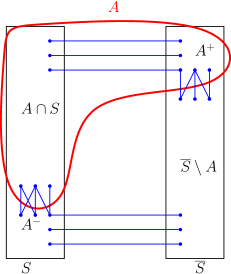
Refer to caption — Figure 1: Illustration of the sets $A$ (red), $S$ , $A^{+}$ and $A^{-}$ , and the edges incident on $A^{+}$ and $A^{-}$ (blue).

The high-level idea is that the edge boundaries of $A^{+}$ and $A^{-}$ consist of $E(A^{-},\overline{S})$ and $E(A^{+},S)$ , which cross the cut $S$ , and $E(A^{-},A\cap S)$ and $E(A^{+},\overline{S}\setminus A)$ , which cross the cut $A$ . Since the former two sets cross the coordinate cut, they have size at most $|A^{+}|+|A^{-}|=O(\epsilon)2^{d-1}$ . Since the latter two sets contribute to the cut $A$ , they cannot be too large, as otherwise the edge-boundary of $A$ would have size significantly larger than $(1+\epsilon)2^{d-1}.$ We now prove this more formally.

Claim 11.

|\partial(A^{+})|+|\partial(A^{-})|\leq|\partial(A)|-|\partial(S)|+2|E(A^{+},S% )|+2|E(A^{-},\overline{S})|.

Proof.

Since $A$ is partitioned into $A\cap S$ and $A^{+}$ , and $V\setminus A$ is partitioned into $A^{-}$ and $\overline{S}\setminus A$ , we have

|\partial(A)|=|E(A\cap S,\overline{S}\setminus A)|+|E(A^{+},A^{-})|+|E(A\cap S% ,A^{-})|+|E(A^{+},\overline{S}\setminus A)|.

Similarly, since $S$ is partitioned into $A\cap S$ and $A^{-}$ , and $\overline{S}$ is partitioned into $A^{+}$ and $\overline{S}\setminus A$ , we have

|\partial(S)|=|E(A\cap S,\overline{S}\setminus A)|+|E(A^{-},A^{+})|+|E(A\cap S% ,A^{+})|+|E(A^{-},\overline{S}\setminus A)|.

Combining, we get

	$\displaystyle\|\partial(A)\|-\|\partial(S)\|$	$\displaystyle=\|E(A^{-},A\cap S)\|+\|E(A^{+},\overline{S}\setminus A)\|-\|E(A\cap S% ,A^{+})\|-\|E(A^{-},\overline{S}\setminus A)\|$
		$\displaystyle\geq\|E(A^{-},A\cap S)\|+\|E(A^{+},\overline{S}\setminus A)\|-\|E(A^{+% },S)\|-\|E(A^{-},\overline{S})\|.$

On the other hand, we have

|\partial(A^{-})|+|\partial(A^{+})|=|E(A^{-},S\cap A)|+|E(A^{-},\overline{S})|% +|E(A^{+},S)|+|E(A^{+},\overline{S}\setminus A)|.

Combining the above two equations yields the claim. $\hfill\vartriangleleft$

To continue, note that the edges in $E(A^{+},S)$ and in $E(A^{-},\overline{S})$ are crossing the coordinate cut $S$ . Since $S$ is a coordinate cut, every vertex can have at most one edge crossing $S$ incident on it. This gives

|E(A^{+},S)|+|E(A^{-},\overline{S})|\leq|A^{+}|+|A^{-}|=|A\triangle S|\leq K% \cdot\epsilon 2^{d-1},

(7)

where the last inequality follows by the lemma assumption. Combining with Claim 11, and recalling from the lemma assumption that $|\partial(A)|\leq(1+\epsilon)|A|\leq(1+\epsilon)2^{d-1}$ , we obtain

$\displaystyle\|\partial(A\triangle S)\|$	$\displaystyle\leq\|\partial(A^{-})\|+\|\partial(A^{+})\|$
	$\displaystyle\leq\|\partial(A)\|-\|\partial(S)\|+2\|E(A^{+},S)\|+2\|E(A^{-},\overline% {S})\|$	by Claim (11)
	$\displaystyle\leq\|\partial(A)\|-\|\partial(S)\|+2K\cdot\epsilon 2^{d-1}$	by Equation (7)
	$\displaystyle\leq(1+\epsilon)2^{d-1}-2^{d-1}+2K\cdot\epsilon 2^{d-1}$	by the lemma assumption
	$\displaystyle=C\cdot\epsilon 2^{d-1},$	for $C=2K+1$

which completes the proof. $\hfill\blacktriangleleft$ With this stronger bound on $\partial(A\triangle S)$ , we can now bound the number of cuts $A$ of size $\partial(A)\leq(1+\epsilon)2^{d-1}$ .

Lemma 12.

Let $S$ be a coordinate cut. The number of sets $A\subseteq Q_{k}$ of size $|A|=2^{d-1}$ such that $|\partial(A)|\leq(1+2\epsilon)2^{d-1}$ and $|A\triangle S|\leq K\cdot\epsilon 2^{d}$ is at most $\exp\left(2^{d}O({\epsilon}/d)\log(d/{\epsilon})\right)$ .

Proof.

Let $A\subseteq Q_{k}$ be of size $|A|=2^{d-1}$ such that $|\partial(A)|\leq(1+2\epsilon)\binom{d-1}{k-1}2^{d-1}$ and $|A\triangle S|\leq K\cdot\epsilon 2^{d}$ . Given $S$ , the set $A$ is uniquely determined by the choice of $A\triangle S$ , so we just need to count the number of possible choices for $A\triangle S$ . Letting $C$ denote the universal constant in Lemma 10, we have

|\partial(A\triangle S)|\leq C\epsilon 2^{d-1}.

On the other hand, by Lemma 5, the minimum cut has size $d$ , so $\partial(A\triangle S)$ is an $\alpha$ -approximate minimum cut with $\alpha=C\frac{\epsilon}{d}2^{d-1}.$ Therefore, by Karger’s cut counting theorem (Theorem 9), the number of choices for $|A\triangle S|$ is at most

2^{C{\epsilon}/d2^{d-1}}\binom{2^{d}}{C{\epsilon}/d2^{d-1}}\leq 2^{C{\epsilon}% /d2^{d-1}}\cdot 2^{H_{2}(C{\epsilon}/d)2^{d}}\leq\exp\left(2^{d}O({\epsilon}/d% )\log(d/{\epsilon})\right).

Here $H_{2}(x)$ denotes the binary entropy function $H_{2}(x)=-x\log x-(1-x)\log(1-x).$ $\hfill\blacktriangleleft$

To bound the deviation of the cut sizes after subsampling, we use the additive Chernoff bound (see e.g., Theorems 1.10.10 and 1.10.11 in [17]).

Theorem 13.

Let $X_{1},\dots,X_{n}$ be independent random variables taking values in $[0,1]$ . Let $X=\sum_{i=1}^{n}X_{i}$ . Let $\lambda\geq 0$ . Then

\Pr[|X-\mathbb{E}[X]|\geq\lambda]\leq 2\exp\Bigr(-\frac{1}{3}\min\{\lambda^{2}% /\mathbb{E}[X],\lambda\}\Bigr).

Applying the Chernoff bound, we show that with high probability, every cut $A$ remains larger than its closest coordinate cut after subsampling.

Lemma 14.

Let $\epsilon>0$ and let $A\subseteq V$ be a set of size $A=2^{d-1}$ such that $(1+\epsilon)|A|\leq E(A,V\setminus A)\leq(1+2\epsilon)|A|.$ Let $S$ be the coordinate cut such that $|A\triangle S|\leq O(\epsilon)2^{d}$ (exists by Lemma 8). Then

\Pr\left[|E^{\prime}(A,V\setminus A)|\geq|E^{\prime}(S,V\setminus S)|+\frac{p% \epsilon}{2}\cdot 2^{d-1}.\right]\geq 1-4e^{-\Omega\left(\epsilon p2^{d-1}% \right)}.

Proof.

Let $E^{+}\coloneqq\partial(A)\setminus\partial(S)$ and let $E^{-}\coloneqq\partial(S)\setminus\partial(A)$ . We have

	$\displaystyle\|E^{\prime}(A,V\setminus A)\|-\|E^{\prime}(S,V\setminus S)\|$	$\displaystyle=\left\|(\partial(A)\setminus\partial(S))\cap E^{\prime}\right\|-% \left\|(\partial(S)\setminus\partial(A))\cap E^{\prime}\right\|$
		$\displaystyle=\|E^{+}\cap E^{\prime}\|-\|E^{-}\cap E^{\prime}\|.$

So we need to bound the probability of the event $|E^{+}\cap E^{\prime}|-|E^{-}\cap E^{\prime}|\geq\frac{p\epsilon}{2}2^{d-1}.$ From the lemma assumption, we have

|E^{+}|-|E^{-}|=|E(A,V\setminus A)|-|E(S,V\setminus S)|\geq(1+\epsilon)|A|-|S|% =\epsilon\cdot 2^{d-1}.

(8)

By Lemma 10, we have

\mathbb{E}[|E^{+}\cap E^{\prime}|]=p|E^{+}|\leq p\cdot O(\epsilon)2^{d}\qquad% \text{and}\qquad\mathbb{E}[|E^{-}\cap E^{\prime}|]=p|E^{-}|\leq p\cdot O(% \epsilon)2^{d}.

Let $\lambda=\frac{p\epsilon}{4}\cdot 2^{d-1}.$ Then $\min\{\lambda,\lambda^{2}/p|E^{-}|\},\min\{\lambda,\lambda^{2}/p|E^{+}|\}\geq% \Omega\left(\epsilon p2^{d-1}\right)$ , so applying the Chernoff bound (Lemma 13), we get

\Pr\left[\Bigr||E^{-}\cap E^{\prime}|-p|E^{-}|\Bigr|\geq\frac{p\epsilon}{4}% \cdot 2^{d-1}\right]\leq 2e^{-\Omega({\epsilon}p2^{d-1})}

and

\Pr\left[\Bigr||E^{+}\cap E^{\prime}|-p|E^{+}|\Bigr|\geq\frac{p\epsilon}{4}% \cdot 2^{d-1}\right]\leq 2e^{-\Omega({\epsilon}p2^{d-1})}.

By a union bound, with probability at least $1-4e^{-\Omega({\epsilon}p2^{d-1})}$ , it holds that

\displaystyle|E^{+}\cap E^{\prime}|-|E^{-}\cap E^{\prime}|

\displaystyle\geq p|E^{+}|-p|E^{-}|-\frac{p\epsilon}{2}\cdot 2^{d-1}\geq p% \epsilon 2^{d-1}-\frac{p\epsilon}{2}\cdot 2^{d-1}=\frac{p\epsilon}{2}\cdot 2^{% d-1},

where the second inequality follows from Equation (8). $\hfill\blacktriangleleft$ We can now show that every sufficiently large cut remains larger than a coordinate cut after subsampling.

Lemma 15.

Let $p\geq\kappa\frac{\log d}{d}$ for a sufficiently large constant $\kappa$ , and let $\epsilon_{0}=d^{-100}$ . Then with probability at least $1-d^{-100}/2$ , the following holds: For every $\epsilon\geq\epsilon_{0}$ and every balanced cut $A$ of size $|E(A,V\setminus A)|=(1+\epsilon)2^{d-1}$ , it holds that

|E^{\prime}(A,V\setminus A)|\geq|E^{\prime}(S,V\setminus S)|+\frac{p\epsilon}{% 2}2^{d-1},

where $S$ is the coordinate cut such that $|A\triangle S|\leq K\cdot\epsilon 2^{d}$ (exists by Lemma 8).

Proof.

Suppose $\kappa\geq 204C/D$ , where $C$ denotes the hidden constant in the $O$ -notation in Lemma 12 and $D$ denotes the hidden constant in the $\Omega$ -notation in Lemma 14. Let $\epsilon_{i}=2^{i}\epsilon_{0}$ for $i=1,\dots\log(2^{d}d/\epsilon_{0})$ . For every coordinate cut $S=S_{j,b}$ with $j\in[d]$ and $b\in\{0,1\}$ , and for every $\epsilon_{i}$ , let $\mathcal{B}(S,\epsilon_{i})$ be the event that there exists a cut $A$ of size $(1+\epsilon_{i})2^{d-1}\leq|E(A,V\setminus A)|\leq(1+2\epsilon_{i})2^{d-1}$ with $|A\triangle S|\leq K\cdot\epsilon_{i}2^{d}$ such that

|E^{\prime}(A,V\setminus A)|<|E^{\prime}(S,V\setminus S)|+\frac{p\epsilon}{2}2% ^{d-1}.

We now show that $\Pr[\mathcal{B}(S,\epsilon_{i})]\leq d^{-102}/8.$ For every cut $A$ of size $|E(A,V\setminus A)|\leq(1+2\epsilon_{i})2^{d-1}$ with $|A\triangle S|\leq K\cdot\epsilon_{i}2^{d}$ , by Lemma 14, we have

\Pr\left[|E^{\prime}(A,V\setminus A)|<|E^{\prime}(S,V\setminus S)|+\frac{p% \epsilon_{i}}{2}2^{d-1}\right]\leq 4\exp\left(-D\epsilon_{i}p2^{d-1}\right).

By Lemma 12, the number of such cuts is at most $\exp\left(2^{d}C\frac{{\epsilon}_{i}}{d}\log(d/{\epsilon}_{i})\right)$ . Therefore, by a union bound, we have
$\displaystyle\Pr[\mathcal{B}(S,\epsilon_{i})]$ $\displaystyle\leq 4\exp\left(-D\epsilon_{i}p2^{d-1}\right)\cdot\exp\left(2^{d}% C\frac{{\epsilon}_{i}}{d}\log(d/{\epsilon}_{i})\right)$ $\displaystyle=4\exp\left(2^{d}\epsilon_{i}\left(C\frac{\log(d/\epsilon_{i})}{d% }-\frac{D\cdot p}{2}\right)\right)$ $\displaystyle\leq 4\exp\left(2^{d}\epsilon_{i}\left(101C\frac{\log d}{d}-% \kappa\frac{D\log d}{2d}\right)\right)$ since $\frac{1}{\epsilon_{i}}\leq\frac{1}{\epsilon_{0}}\leq d^{100}$ and $p\geq\frac{\kappa\log d}{d}$ $\displaystyle\leq 4\exp\left(-2^{d}\epsilon_{i}C\frac{\log d}{d}\right)$ since $\kappa\geq 204C/D$ $\displaystyle=4\exp\left(-2^{d}/\mathrm{poly}\left(d\right)\right)$ since $\epsilon_{i}\geq\epsilon_{0}=d^{-100}$ $\displaystyle<\frac{1}{8d^{102}}$ for $d$ sufficiently large.

Finally, taking a union bound over the $2d$ possible choices of $S$ and the $\log(2^{d}/\epsilon_{0})\leq 2d$ possible choices for $i$ , gives the lemma. $\hfill\blacktriangleleft$ Lemma 15 implies that the sparsest cut after sampling is close in Hamming distance to a coordinate cut. However, since the objective value of (1) is a sum $\sum_{i}|E^{\prime}(A_{i},V\setminus A_{i})|$ , we need to exclude the possibility that the optimal solution includes a large cut $|E^{\prime}(A_{i},V\setminus A_{i})|$ due to the other cuts being surprisingly sparse. Corollary 16 handles this.

Corollary 16.

Conditioned on the success of the event in Lemma 15, for every balanced cut $A\subseteq V$ , it holds that

|E^{\prime}(A,V\setminus A)|\geq|E^{\prime}(S,V\setminus S)|-C\epsilon_{0}2^{d% -1},

where $S$ is the coordinate with the smallest hamming distance to $A$ , $C$ is a universal constant, and $\epsilon_{0}=d^{-100}$ .

Proof.

Let $C$ be he universal constant from Lemma 10. Let $A\subseteq V$ be a cut of size $|E(A,V\setminus A)|=(1+\epsilon)2^{d-1},$ and let $S$ be the coordinate cut with the smallest Hamming distance to $A$ . By Lemma 8, we have $|A\triangle S|\leq K\cdot\epsilon 2^{d-1}$ . Consider two cases depending on $\epsilon$ .

Suppose $\epsilon\geq\epsilon_{0}$ . Then by Lemma 15, we have $|E^{\prime}(A,V\setminus A)|\geq|E^{\prime}(S,V\setminus S)|$ , so we are done.

Suppose instead that $\epsilon<\epsilon_{0}$ . Then by Lemma 10, we have $|\partial(A)\triangle\partial(S)|\leq C\epsilon_{0}2^{d-1}$ , which gives

|E^{\prime}(A,V\setminus A)|\geq|E^{\prime}(S,V\setminus S)|-|\partial(A)% \triangle\partial(S)|\geq|E^{\prime}(S,V\setminus S)|-C\epsilon_{0}2^{d-1}.\

$\hfill\blacktriangleleft$ We also need to bound the optimal value of (1).

Lemma 17.

Let $K$ be the universal constant from Lemma 8. With probability at least $1-d^{-100}/2$ , all coordinate cuts $S_{j,b}$ satisfy

\left||E^{\prime}(S_{j,b},V\setminus S_{j,b})|-p2^{d-1}\right|\geq\frac{p}{100% Kd}2^{d-1},

and in particular, the optimal value of (1) is at most $\left(d+\frac{1}{100K}\right)2^{d-1}p$ .

Proof.

Fix a coordinate cut $S_{j,b}$ . Then $\mathbb{E}[|E^{\prime}(S_{j,b},V\setminus S_{j,b})|]=2^{d-1}p$ , so applying the Chernoff bound (Lemma 13) with $\lambda=\frac{1}{100Kd}2^{d-1}p$ , we obtain

	$\displaystyle\Pr\left[\left\|\|E^{\prime}(S_{j,b},V\setminus S_{j,b})\|-p2^{d-1}% \right\|\geq\frac{p}{100Kd}2^{d-1}\right]$	$\displaystyle\leq\exp\left(-\frac{1}{3}\frac{1}{100^{2}K^{2}d^{2}}p2^{d-1}\right)$
		$\displaystyle=\exp\left(-2^{d}/\mathrm{poly}\left(d\right)\right)$
		$\displaystyle\leq d^{-101}/2.$

By a union bound over the $d$ coordinate cuts, the above equation holds simultaneously for all $S_{j,b}$ with probability at least $1-d^{-100}/2.$ If this holds, then, since $\{S_{j,b}:j\in[d],b=0\}$ is a feasible solution to (1), the optimal value of (1) is at most

\sum_{j}|E^{\prime}(S_{j,0},V\setminus S_{j,0})|\leq d\cdot\left(1+\frac{1}{10% 0Kd}\right)2^{d-1}p=\left(d+\frac{1}{100K}\right)2^{d-1}p.\

$\hfill\blacktriangleleft$

Finally, we put everything together to prove Theorem 1.

Proof of Theorem 1.

The algorithm solves the optimization problem

$\displaystyle\min$	$\displaystyle\sum_{i=1}^{d}\|E^{\prime}(A_{i},V\setminus A_{i})\|\qquad\text{% subject to}$		(1)
	$\displaystyle\|A_{i}\|=2^{d-1}$	$\displaystyle\forall i,$
	$\displaystyle\|A_{i}\triangle A_{j}\|=2^{d-1}$	$\displaystyle\forall i\neq j$

and outputs the optimal solution $A_{1},\dots,A_{d}$ .

Running time.

We can solve this program by enumerating all feasible families of cuts, of which there are at most $\left(\binom{2^{d}}{2^{d-1}}\right)^{d}=2^{O\left(2^{d}d\right)}=2^{O(n\log n)}$ and computing the corresponding edge counts, so the running time is $2^{O(n\log n)}$ .

Correctness.

Condition on the success of the events in Lemma 15 and Lemma 17. By a union bound, this occurs with probability at least $1-d^{-100}.$

Let $\{A_{i}\}_{i\in[d]}$ be the optimal solution to (1). For every $i\in[d]$ , let $S_{i}$ denote the coordinate cut with the smallest Hamming distance to $A_{i}$ . We start by proving that this is a matching, i.e., that the set $\{S_{i}\}_{[d]}$ consists of $d$ different coordinate cuts. Suppose not. Then $S_{i}=S_{j}$ or $S_{i}=\overline{S}_{j}$ for some $i\neq j$ . If $S_{i}=S_{j}=S$ , then by triangle inequality,

|A_{i}\triangle S|+|A_{j}\triangle S|\;\geq\;|A_{i}\triangle A_{j}|\;=\;2^{d-1},

so either $|A_{i}\triangle S_{i}|\geq 2^{d-2}$ or $|A_{j}\triangle S_{j}|\geq 2^{d-2}.$ If instead $S_{i}=\overline{S}_{j}=S$ , then again by triangle inequality,

|A_{i}\triangle S|+|A_{j}\triangle\overline{S}|=|A_{i}\triangle S|+2^{d}-|A_{j% }\triangle S|\geq 2^{d}-|A_{i}\triangle A_{j}|=2^{d-1},

so again either $|A_{i}\triangle S_{i}|\geq 2^{d-2}$ or $|A_{j}\triangle S_{j}|\geq 2^{d-2}$ .

Let $i$ be the index such that $|A_{i}\triangle S_{i}|\geq 2^{d-2}$ . Applying Lemma 8 with $\epsilon=1/4$ gives $|E(A_{i},V\setminus A_{i})|\geq(1+\frac{1}{4K})2^{d-1}$ , where $K$ is the universal constant from Lemma 8. Therefore, by Lemma 15 and Lemma 17, we have

$\displaystyle\|E^{\prime}(A_{i},V\setminus A_{i})\|$	$\displaystyle\geq\|E^{\prime}(S_{i},V\setminus S_{i})\|+\frac{p}{8K}2^{d-1}$	by Lemma 15
	$\displaystyle\geq\left(1-\frac{1}{100K}\right)p2^{d-1}+\frac{p}{8K}2^{d-1}$	by Lemma 17
	$\displaystyle\geq\left(1+\frac{1}{10K}\right)p2^{d-1}.$

Furthermore, letting $C$ be the universal constant from Corollary 16, for every $j\neq i$ , we have

$\displaystyle\|E^{\prime}(A_{j},V\setminus A_{j})\|$	$\displaystyle\geq\|E^{\prime}(S_{j},V\setminus S_{j})\|-C\epsilon_{0}2^{d-1}$	by Corollary 16
	$\displaystyle\geq\left(1-\frac{1}{100Kd}\right)p2^{d-1}-C\epsilon_{0}2^{d-1}$	by Lemma 17
	$\displaystyle>\left(1-\frac{1}{50Kd}\right)p2^{d-1}$	since $\epsilon_{0}=d^{-100}\ll\frac{p}{Kd}$ .

But then summing over all $j\in[d]$ gives

	$\displaystyle\sum_{j\in[d]}\|E^{\prime}(A_{j},V\setminus A_{j})\|$	$\displaystyle\geq\left(1+\frac{1}{10K}\right)p2^{d-1}+(d-1)\left(1-\frac{1}{50% Kd}\right)p2^{d-1}$
		$\displaystyle>\left(d+\frac{1}{100K}\right)p2^{d-1},$

which is a contradiction, since objective value of (1) is at most $\left(d+\frac{1}{100K}\right)p2^{d}$ , by Lemma 17. Thus, the set $\{S_{i}\}_{i\in[d]}$ must contain $d$ distinct coordinate cuts.

So now suppose that we have a matching, i.e. that the set $\{S_{i}\}_{i\in[d]}$ contains $d$ distinct coordinate cuts. Then $\{S_{i}\}_{i\in[d]}$ is a feasible solution to (1). Recall that $K$ is the universal constant from Lemma 8 and $C$ is the universal constant from Corollary 16. Let $L\geq 2K\cdot C$ , and suppose for contradiction that

|A_{i}\triangle S_{i}|\geq L\epsilon_{0}d2^{d-1}/p

for some $i\in[d]$ . Applying Lemma 8 with $\epsilon=\frac{L}{K}\epsilon_{0}d/p$ , gives

|E(A_{i},V\setminus A_{i})|\geq\left(1+\frac{L}{K}\epsilon_{0}d/p\right)2^{d-1% }\geq\left(1+2C\epsilon_{0}d/p\right)2^{d-1},

where the last inequality follows by choice of $L$ . So by Lemma 15, we have

|E^{\prime}(A_{i},V\setminus A_{i})|\geq|E^{\prime}(S_{i},V\setminus S_{i})|+C% \epsilon_{0}d2^{d-1}.

But then, by Corollary 16, we have
$\displaystyle\sum_{j\in[d]}|E^{\prime}(A_{j},V\setminus A_{j})|$ $\displaystyle\geq|E^{\prime}(S_{i},V\setminus S_{i})|+C\epsilon_{0}d2^{d-1}+% \sum_{j\neq i}|E^{\prime}(A_{j},V\setminus A_{j})|$ $\displaystyle\geq|E^{\prime}(S_{i},V\setminus S_{i})|+Cd\epsilon_{0}2^{d-1}+% \sum_{j\neq i}|E^{\prime}(S_{j},V\setminus S_{j})|-(d-1)C\epsilon_{0}2^{d-1}$ $\displaystyle>\sum_{j=1}^{d}|E^{\prime}(S_{j},V\setminus S_{j})|,$

which contradicts the optimality of $\{A_{i}\}_{i\in[d]}$ , since $\{S_{i}\}_{i\in[d]}$ is a feasible solution. Therefore, we conclude that with probability at least $1-d^{-100}$ , it holds that $|A_{i}\triangle S_{i}|\leq L\epsilon_{0}d2^{d-1}/p\leq 2^{d-1}/\mathrm{poly}% \left(d\right)$ for all $i$ . $\hfill\blacktriangleleft$

3 Proof of Theorem 4

In this section, we prove Theorem 4, restated below for the convenience of the reader. See 4

The proof follows the same overall strategy as Theorem 1. The algorithm solves to following optimization problem and outputs the optimal solution.

$\displaystyle\min$	$\displaystyle\sum_{i=1}^{d}\|E^{\prime}(A_{i},V\setminus A_{i})\|\qquad\text{% subject to}$		(9)
	$\displaystyle\|A_{i}\|=\frac{\|V\|}{2}$	$\displaystyle\forall i,$
	$\displaystyle\|A_{i}\triangle A_{j}\|=\frac{\|V\|}{2}$	$\displaystyle\forall i\neq j.$

We want to use the FKN Theorem (Theorem 7) to show that every sparse cut is close to a coordinate cut, and then use Karger’s cut-counting theorem (Theorem 9) to union bound over all cuts. In the $k$ -distance cube, every vertex has degree $\binom{d}{k}$ , and for every coordinate cut $S_{j,b}$ and every vertex $v\in V$ , exactly $\binom{d-1}{k-1}$ of the edges incident on $v$ cross the cut $S_{j,b}$ . These higher degrees allow for better concentration bounds, which is why we can achieve exact recovery. It is important to note that when $k$ is even, the $k$ -distance cube $Q_{d,k}$ has at least two components, corresponding to the vertices with odd Hamming weight, and the vertices with even Hamming weight.

Definition 18 (Component of $Q_{d,k}$ ).

Let $Q_{d,k}^{E}$ , $Q_{d,k}^{O}\subseteq Q_{d,k}$ be the subgraphs induced by

\{x\in\{0,1\}^{d}:|x|\equiv 0\pmod{2}\},\qquad\text{and}\qquad\{x\in\{0,1\}^{d% }:|x|\equiv 1\pmod{2}\},

respectively. We say that $Q\subseteq Q_{d,k}$ is an component of $Q_{d,k}$ if

$\blacksquare$

$Q=Q_{d,k}$ and $k$ is odd, or
$\blacksquare$

$Q\in\{Q_{d,k}^{E},Q_{d,k}^{O}\}$ and $k$ is even.

We say that a cut $S$ is a coordinate cut in $Q$ if $S=S_{j,b}\cap Q$ for some coordinate cut $S_{j,b}.$

Later, in Remark 23, we will see that when $d$ is sufficiently large, the components of $Q_{d,k}$ are exactly the connected components.

We start by analyzing the spectrum of the $k$ -distance cube $Q_{d,k}$ . Known results for the Hamming association scheme (see e.g. Theorem 5, Chapter 21 in [28]) show that the eigenvalues $\{\mu_{S}\}_{S\subseteq[d]}$ of the adjacency matrix of $Q_{d,k}$ are given by binary Krawtchouk polynomials

\mu_{S}=\mathcal{K}_{k}(|S|;d)\coloneqq\sum_{j=0}^{k}(-1)^{j}\binom{|S|}{j}% \binom{d-|S|}{k-j}.

Therefore, the eigenvalues $\{\lambda_{S}\}_{S\subseteq[d]}$ of the Laplacian $\mathcal{L}$ satisfy

\lambda_{S}=\binom{d}{k}-\mu_{S}=2\sum_{\begin{subarray}{c}j\in[k]:\\ j\text{ odd}\end{subarray}}\binom{|S|}{j}\binom{d-|S|}{k-j}.

We include a direct calculation of the eigenvalues $\lambda_{S}$ in the full version for completeness.

Lemma 19 (Eigenvalues of $Q_{d,k}$ ).

Let $k$ be an integer, and let $\mathcal{L}$ be the unnormalized Laplacian of $Q_{d,k}$ . Then the Fourier characters $\chi_{S}$ form an eigenbasis of $\mathcal{L}$ , with corresponding eigenvalues

\lambda_{S}=2\sum_{\begin{subarray}{c}j\in[k]:\\ j\text{ odd}\end{subarray}}\binom{|S|}{j}\binom{d-|S|}{k-j}.

(10)

Using the above lemma, we can write the size of any cut in $Q_{d,k}$ in terms of the Fourier coefficients of its indicator function.

Lemma 20.

Let $Q_{d,k}$ be the $d$ -dimensional $k$ -distance hypercube, and let $Q=(V,E)$ be component of $Q$ (as per Definition 18). Let $A\subseteq V$ , and let $f\colon V\rightarrow\{0,1\}$ denote the indicator function on $A$ . Then

|E(A,V\setminus A)|=2^{d}\sum_{S\subseteq[d]}\lambda_{S}\widehat{f}(S)^{2}.

Proof.

Since there are no edges between $Q_{d,k}^{E}$ and $Q_{d,k}^{O}$ , we can use the unnormalized Lapacian $\mathcal{L}$ of the entire graph $Q_{d,k}$ to express the cut size of $A$ as

|E(A,V\setminus A)|=\sum_{\{x,y\}\in E}(f(x)-f(y))^{2}=f^{\top}\mathcal{L}f,

(11)

On the other hand, expanding $f$ in the Fourier basis, we have $f=\sum_{S\subseteq[d]}\widehat{f}(S)\chi_{S}.$ By Lemma 19, every Fourier character $\chi_{S}$ is an eigenvector of $\mathcal{L}$ with eigenvalue $\lambda_{S}$ , which gives

f^{\top}\mathcal{L}f=\left(\sum_{S\subseteq d}\widehat{f}(S)\chi_{S}\right)^{% \top}\mathcal{L}\left(\sum_{S\subseteq d}\widehat{f}(S)\chi_{S}\right)=\sum_{S% \subseteq[d]}\lambda_{S}\widehat{f}(S)^{2}\|\chi_{S}\|^{2}_{2}=2^{d}\sum_{S% \subseteq[d]}\lambda_{S}\cdot\widehat{f}(S)^{2}.

(12)

Combining Equations (11) and (12) gives the lemma. $\hfill\blacktriangleleft$

To argue that every sparse cut places most of its Fourier mass on the first two levels, we first need to argue that the eigenvalues $\lambda_{S}$ with $|S|>1$ are large compared to those with $|S|=1$ .

Lemma 21.

Let $k$ be a positive integer, and let $d=d(k)$ be sufficiently large. Denote by $\lambda_{1}$ the eigenvalue corresponding to sets $S\subseteq[d]$ of size $|S|=1$ . Then:

$\blacksquare$

If $k$ is odd, then for every $S\subseteq[d]$ with $|S|\geq 2$ , it holds that $\lambda_{S}\geq\tfrac{3}{2}\,\lambda_{1}.$
$\blacksquare$

If $k$ is even, then for every $S\subseteq[d]$ with $2\leq|S|\leq d-2$ , it holds that $\lambda_{S}\geq\tfrac{3}{2}\,\lambda_{1}$ , and for every $S\subseteq[d]$ with $|S|=d-1$ , it holds that $\lambda_{S}=\lambda_{1}$ .

The proof of Lemma 21 is included in the full version. Using the spectral gap established in Lemma 21, we will show that every sparse cut places most of its Fourier mass on the first two levels. As a first step, we derive a lower bound on the expansion of a cut in terms of the higher-level Fourier coefficients.

Lemma 22.

Let $k$ be an integer, let $d$ be sufficiently large, and let $Q=(V,E)$ be a component of $Q_{d,k}$ (as per Definition 18). Let $A\subseteq Q$ with $|A|\leq\frac{|V|}{2}$ , and let $f:\{0,1\}^{d}\rightarrow\{0,1\}$ be the indicator function on $A$ .

$\blacksquare$

If $k$ is odd, then

$|E(A,V\setminus A)|\geq\binom{d-1}{k-1}\left(|A|+2^{d}\sum_{S\subseteq[d]:|S|% \geq 2}\widehat{f}(S)^{2}\right).$
$\blacksquare$

If $k$ is even, then

$|E(A,V\setminus A)|\geq\binom{d-1}{k-1}\left(|A|+2^{d}\sum_{S\subseteq[d]:2% \leq|S|\leq d-2}\widehat{f}(S)^{2}\right).$

$\blacktriangleright$ Remark 23 (Coordinate cuts are sparsest cuts).

Recall that the coordinate cuts have expansion $\binom{d-1}{k-1}$ . Lemma 22 shows that every cut in the component $Q$ has expansion at least this large, and hence the coordinate cuts are the sparsest cuts. This also implies that the components of $Q_{d,k}$ (as per Definition 18) are exactly the connected components of $Q_{d,k}$ .

Proof.

We prove the lemma for the case when $k$ is odd. The case when $k$ is even is similar and is included in the full version. We have

|A|=\sum_{x\in V}f(x)^{2}=2^{d}\sum_{S\subseteq[d]}\widehat{f}(S)^{2}

(13)

and, since $\widehat{f}(\emptyset)=2^{-d}\sum_{x\in V}f(x)=2^{-d}|A|$ , we have

\widehat{f}(\emptyset)^{2}=2^{-2d}|A|.

(14)

Denote by $\lambda_{1}=2\binom{d-1}{k-1}$ the eigenvalue corresponding to sets $S\subseteq[d]$ of size $|S|=1$ . Also note from (10), that $\lambda_{\emptyset}=0$ . Combining Lemma 20, together with Equations (13) and (14) gives
$\displaystyle|E(A,V\setminus A)|$ $\displaystyle=2^{d}\sum_{S\subseteq[d]}\lambda_{S}\widehat{f}(S)^{2}$ by Lemma 20 $\displaystyle=2^{d}\sum_{|S|\geq 2}\left(\lambda_{S}-\lambda_{1}\right)% \widehat{f}(S)^{2}+2^{d}\lambda_{1}\sum_{S\subseteq[d]}\widehat{f}(S)^{2}-2^{d% }\lambda_{1}\widehat{f}(\emptyset)^{2}$ $\displaystyle\geq 2^{d}\frac{\lambda_{1}}{2}\sum_{|S|\geq 2}\widehat{f}(S)^{2}% +2^{d}\lambda_{1}\sum_{S\subseteq[d]}\widehat{f}(S)^{2}-2^{d}\lambda_{1}% \widehat{f}(\emptyset)^{2}$ by Lemma 21 $\displaystyle=\frac{\lambda_{1}}{2}\left(2^{d}\sum_{|S|\geq 2}\widehat{f}(S)^{% 2}+|A|+2|A|\left(\frac{1}{2}-\frac{|A|}{2^{d}}\right)\right)$ by (13) and (14) $\displaystyle\geq\binom{d-1}{k-1}\left(2^{d}\sum_{|S|\geq 2}\widehat{f}(S)^{2}% +|A|\right).$

Here the last inequality uses that $1/2-2^{-d}|A|\geq 0$ , by the assumption. $\hfill\blacktriangleleft$

As a corollary of Lemma 22, we get that sparse cuts place almost all of their Fourier mass on the first two levels (and, in the even- $k$ case, also on the top two levels).

Corollary 24.

Let $k$ be an integer, let $d$ be sufficiently large and let $Q=(V,E)$ be a component of $Q_{d,k}$ (as per Definition 18). Let $A$ be a subset $Q$ with $|A|\leq\frac{|V|}{2}$ and suppose that $|E(A,V\setminus A)|\leq(1+\epsilon)\binom{d-1}{k-1}|A|$ . Let $f$ denote the indicator function of $A$ . Then

$\blacksquare$

If $k$ is odd, then $\sum_{|S|\geq 2}\widehat{f}(S)^{2}\leq\frac{\epsilon}{2}.$
$\blacksquare$

If $k$ is even, then $\sum_{2\leq|S|\leq d-2}\widehat{f}(S)^{2}\leq\frac{\epsilon}{2}.$

Proof.

We prove the lemma for the case when $k$ is odd. The case when $k$ is even is similar and is included in the full version. By Lemma 22, we have

(1+\epsilon)\binom{d-1}{k-1}|A|\geq|E(A,V\backslash A)|\geq\binom{d-1}{k-1}% \left(|A|+2^{d}\sum_{S\subseteq[d]:|S|\geq 2}\widehat{f}(S)^{2}\right),

which gives

\epsilon 2^{d-1}\geq\epsilon|A|\geq 2^{d}\sum_{S\subseteq[d]:|S|\geq 2}% \widehat{f}(S)^{2}.\

$\hfill\blacktriangleleft$ We now wish to apply the FKN theorem (Theorem 7) to argue that every sparse cut must be close to a coordinate cut. We can do that in the case when $k$ is odd. However, when $k$ is even, we are in a slightly different setting: First, the function $f$ is only supported on one of the connected components, and second, $f$ puts most of its Fourier mass on both the bottom two and the top two levels. Therefore, we need to extend the FKN theorem to the case of even $k$ .

Lemma 25 (FKN theorem for even $k$ ).

Let $\mathbbm{1}_{E}$ denote the indicator function of the even component $Q_{d}^{E}\coloneqq\{x\in\{0,1\}^{d}:|x|\equiv 0\pmod{2}\}$ . Suppose that $f\colon\{0,1\}^{d}\rightarrow\{0,1\}$ is a boolean function supported on $Q_{d}^{E}$ such that $\|f\|_{2}^{2}=\frac{1}{4}$ and $\sum_{2\leq|S|\leq d-2}\widehat{f}(S)^{2}\leq\delta$ . Then there exists an index $i\in[d]$ such that $\|\mathbbm{1}_{E}\cdot(f(x_{1},x_{2},\dots,x_{d})-x_{i})\|\leq K\delta$ or $\|\mathbbm{1}_{E}\cdot(f(x_{1},x_{2},\dots,x_{d})-(1-x_{i}))\|\leq K\delta$ . Here $K$ is an absolute constant.

The proof is included in the full version. We can now argue that sparse cuts are close to coordinate cuts.

Lemma 26 (Sparse cuts are close to coordinate cuts).

Let $k$ be an integer and let $d=d(k)$ be sufficiently large. Let $Q=(V,E)$ be a component of $Q_{d,k}$ (as per Definition 18). Suppose $A\subseteq Q$ with $|A|=\frac{|V|}{2}$ . If $|E(A,V\setminus A)|\leq(1+\epsilon)\binom{d-1}{k-1}|A|$ , then there exists a coordinate cut $S$ in $Q$ (as per Definition 18) such that

|A\triangle S|\leq K\cdot\epsilon 2^{d}.

Here $K$ is an absolute constant.

Proof.

If $k$ is odd, then the lemma follows from Corollary 24 and the FKN Theorem (Theorem 7).

If $k$ is even, then we can without loss of generality assume that $f$ is supported on the even component, and the lemma follows from Corollary 24 and Lemma 25. $\hfill\blacktriangleleft$

Next, we want to apply Karger’s cut-counting theorem (Theorem 9) and a Chernoff bound (Lemma 13). Similarly to the proof of Theorem 1, we need to establish a strong bound on the size of $\partial(A)\triangle\partial(S)$ and $\partial(A\triangle S)$ .

Lemma 27.

Let $Q=(V,E)$ be component of $Q_{d,k}$ (as per Definition 18) and let $A\subseteq Q$ be a set with $|A|\leq\frac{|V|}{2}$ and $|\partial(A)|\leq(1+\epsilon)\binom{d-1}{k-1}|A|$ . Let $S$ be a coordinate cut in $Q$ with $|A\triangle S|\leq O(\epsilon)2^{d}$ (exists by Lemma 26). Then

|\partial(A)\triangle\partial(S)|\leq|\partial(A\triangle S)|\leq O(\epsilon)% \binom{d-1}{k-1}|A|.

The proof is almost identical to the proof of Lemma 10, and is included in the full version. In order to apply Karger’s cut-counting theorem, we also need to establish the size of the minimum cuts.

Lemma 28 (The singleton cuts are min-cuts).

Let $k$ be an integer, and let $d$ be sufficiently large. Let $Q=(V,E)$ be a component of $Q_{d,k}$ (as per Definition 18). Then

\min_{A\subseteq V:1\leq|A|\leq|V|/2}|E(A,V\setminus A)|=\binom{d}{k}.

Proof.

If $|A|=1$ , then $|E(A,V\setminus A)|=\binom{d}{k}.$ For the rest of the proof, we consider $2\leq|A|\leq|V|/2$ and split into two cases according to $|A|$ .

Case 1: $|A|\geq\binom{d}{k}/\binom{d-1}{k-1}$ .

By Lemma 22, we have

|E(A,V\setminus A)|\geq\binom{d-1}{k-1}|A|\geq\binom{d}{k}.

Case 2: $2\leq|A|<\binom{d}{k}/\binom{d-1}{k-1}$ .

Every vertex in $Q$ has degree $\binom{d}{k}$ . A vertex in $A$ can have at most $|A|-1$ neighbors in $|A|$ , so it must have at least $\binom{d}{k}-|A|+1$ edges to $V\setminus A$ . Summing over all vertices in $A$ , we obtain

|E(A,V\setminus A)|\geq|A|\cdot\left(\binom{d}{k}-|A|+1\right)=\left(\binom{d}% {k}-|A|\right)\left(|A|-1\right)+\binom{d}{k}>\binom{d}{k},

where the last inequality follows from $2\leq|A|\leq\binom{d}{k}/\binom{d-1}{k-1}<\binom{d}{k}$ . $\hfill\blacktriangleleft$ We can now apply Karger’s cut-counting theorem to count the number of cuts of size $(1+\epsilon)\binom{d-1}{k-1}2^{d-1}$ .

Lemma 29.

Let $Q=(V,E)$ be a component of $Q_{d,k}$ (as per Definition 18), and let $S$ be a coordinate in $Q$ . The number of sets $A\subseteq Q$ of size $|A|\leq\frac{|V|}{2}$ such that $|E(A,V\setminus A)|\leq(1+2\epsilon)\binom{d-1}{k-1}|A|$ and $|A\triangle S|\leq O(\epsilon)2^{d}$ is at most $\exp\left(2^{d}O({\epsilon}/d)\log(d/{\epsilon})\right)$ .

Proof.

Given $S$ , the set $A$ is uniquely determined by the choice of $A\triangle S$ , so we just need to count the number of possible choices for $A\triangle S$ . Let $C$ denote the hidden constant in the big $O$ -notation in Lemma 27. By Lemma 27, we have

|\partial(A\triangle S)|\leq C\cdot\epsilon\binom{d-1}{k-1}2^{d-1}.

By Lemma 28, the minimum cut has size $\binom{d}{k}$ , so $\partial(A\triangle S)$ is an $\alpha$ -approximate minimum cut with $\alpha=C\epsilon\binom{d-1}{k-1}2^{d-1}/\binom{d}{k}=C\epsilon 2^{d-1}/d$ . Therefore, by Karger’s cut counting theorem (Theorem 9), the number of choices for $|A\triangle S|$ is at most

2^{C{\epsilon}/d2^{d-1}}\binom{2^{d}}{C{\epsilon}/2^{d-1}}\leq 2^{C{\epsilon}/% d2^{d-1}}\cdot 2^{H_{2}(C{\epsilon}/d)2^{d}}\leq\exp\left(2^{d}O({\epsilon}/d)% \log(d/{\epsilon})\right).

Here $H_{2}(x)$ denotes the binary entropy function $H_{2}(x)=-x\log x-(1-x)\log(1-x).$ $\hfill\blacktriangleleft$

Lemma 30.

Let $Q=(V,E)$ be a component of $Q_{d,k}$ (as per Definition 18), and let $A\subseteq Q$ be a set with $|A|=\frac{|V|}{2}$ and $(1+\epsilon)\binom{d-1}{k-1}|A|\leq E(A,V\setminus A)\leq(1+2\epsilon)\binom{d% -1}{k-1}|A|.$ Let $S$ be the coordinate cut in $Q$ such that $|A\triangle S|\leq O(\epsilon)2^{d}$ (exists by Lemma 26). Then

\Pr\left[|E^{\prime}(A,V\setminus A)|\geq|E^{\prime}(S,V\setminus S)|+\frac{p% \epsilon}{2}\binom{d-1}{k-1}\frac{|V|}{2}\right]\geq 1-4\exp\left(-\Omega(% \epsilon pd^{k-1}2^{d-1})\right).

The proof is similar to Lemma 14, and is included in the full version.

Lemma 31.

Let $Q=(V,E)$ be a component of $Q_{d,k}$ (as per Definition 18). Suppose $p=\kappa\frac{\log d}{d^{k-1}}$ for a sufficiently large constant $\kappa$ , and let $\epsilon_{0}=2^{-d}/K$ , where $K$ is the universal constant from Lemma 26. Then with probability at least $1-d^{-100}/2$ , the following holds: For every $\epsilon\geq\epsilon_{0}$ , and every balanced cut $A\subseteq Q$ of size $|E(A,V\setminus A)|=(1+\epsilon)\binom{d-1}{k-1}\frac{|V|}{2}$ , it holds that

|E^{\prime}(A,V\setminus A)|\geq|E^{\prime}(S,V\setminus S)|+\frac{p\epsilon}{% 2}\binom{d-1}{k-1}\frac{|V|}{2},

where $S$ is the coordinate cut in $Q$ such that $|A\triangle S|\leq K\cdot\epsilon 2^{d}$ (exists by Lemma 26).

Proof.

Let $C$ be the hidden constant in the $O$ -notation in Lemma 29 and let $D$ be the hidden constant in the $\Omega$ -notation in Lemma 30. Suppose that $\kappa$ is a sufficiently large constant. Let $\epsilon_{i}=2^{i}\epsilon_{0}$ for $i=1,\dots\log(2^{d}/\epsilon_{0})$ . For every coordinate cut $S=S_{j,b}\cap Q$ with $j\in[d]$ and $b\in\{0,1\}$ , and for every $\epsilon_{i}$ , let $\mathcal{B}(S,\epsilon_{i})$ be the event that there exists a balanced cut $A\subseteq Q$ of size $(1+\epsilon_{i})|A|\leq|E(A,V\setminus A)|\leq(1+2\epsilon_{i})\binom{d-1}{k-1% }|A|$ with $|A\triangle S|\leq K\cdot\epsilon 2^{d}$ such that

|E^{\prime}(A,V\setminus A)|<|E^{\prime}(S,V\setminus S)|+\frac{p\epsilon_{i}}% {2}\binom{d-1}{k-1}\frac{|V|}{2}.

We now show that $\Pr[\mathcal{B}(Q,\epsilon_{i})]\leq d^{-102}/8.$ For every balanced cut $A$ of size $|E(A,V\setminus A)|\leq(1+2\epsilon_{i})\binom{d-1}{k-1}|A|$ with $|A\triangle S|\leq O(\epsilon_{i})2^{d}$ , by Lemma 30, we have

\Pr\left[|E^{\prime}(A,V\setminus A)|<|E^{\prime}(S,V\setminus S)|+\frac{p% \epsilon_{i}}{2}\binom{d-1}{k-1}\frac{|V|}{2}\right]\leq 4\exp\left(-D\epsilon% _{i}pd^{k-1}2^{d}\right).

By Lemma 29, the number of such cuts is at most $\exp\left(2^{d}C{\epsilon}_{i}/d\log(d/{\epsilon}_{i})\right)$ . Therefore, by a union bound, we have
$\displaystyle\Pr[\mathcal{B}(S,\epsilon_{i})]$ $\displaystyle\leq 4\exp\left(-D\epsilon_{i}pd^{k-1}2^{d}\right)\cdot\exp\left(% 2^{d}C{\epsilon}_{i}/d\log(d/{\epsilon}_{i})\right)$ $\displaystyle=4\exp\left(2^{d}\epsilon_{i}\left(C\log(d/\epsilon_{i})/d-Dpd^{k% -1}/2\right)\right)$ $\displaystyle\leq 4\exp\left(2^{d}\epsilon_{i}\left(C\log d\log K-D\kappa\log d% /2\right)\right),\text{ since $\log(1/\epsilon_{i})\leq\log(1/\epsilon_{0})=d% \log K$}$ $\displaystyle\leq 4\exp\left(-103\log d\right),\qquad\qquad\qquad\qquad\text{% for $\kappa$ sufficiently large, since $\epsilon_{0}=2^{-d}/K$}$ $\displaystyle\leq d^{-102}/8.$

Taking a union bound over the $2d$ possible choices of $S$ and the $\log(2^{d}/\epsilon_{0})\leq 2d$ possible choices for $i$ , we get the claim for $\epsilon\geq\epsilon_{0}$ . $\hfill\blacktriangleleft$

Corollary 32.

Conditioned on the success of the event in Lemma 31, for every balanced cut $A\subseteq Q$ it holds that

|E^{\prime}(A,V\setminus A)|\geq|E^{\prime}(S,V\setminus S)|.

Proof.

Let $A$ be a balanced cut of size $|E(A,V\setminus A)|=(1+\epsilon)\binom{d-1}{k-1}|V|$ . If $\epsilon\geq\epsilon_{0}$ , then we are done by Lemma 31. If instead $\epsilon<\epsilon_{0}$ , then $|E(A,V\setminus A)|<(1+\epsilon_{0})\binom{d-1}{k-1}|A|$ , so by Lemma 26, there exists a coordinate cut $S$ such that

|A\triangle S|<K\epsilon_{0}2^{d-1}\leq 1,

where the last inequality follows by the setting $\epsilon_{0}=2^{-d}/K$ . But then $A$ is equal to $S$ , so we are done. $\hfill\blacktriangleleft$

Lemma 33.

Let $K$ be the universal constant from Lemma 26. With probability at least $1-d^{-100}/2$ , all coordinate cuts $S$ in $Q$ satisfy

\left||E^{\prime}(S,V\setminus S)|-p\binom{d-1}{k-1}2^{d-1}\right|\geq\frac{p}% {100Kd}\binom{d-1}{k-1}\frac{|V|}{2},

and in particular, the optimal value of (9) is at most $\left(d+\frac{1}{100K}\right)\binom{d-1}{k-1}2^{d-1}p$ .

The proof of Lemma 33 is almost identical to the proof of Lemma 17, and is included in the full version.

Proof of Theorem 4.

The algorithm solves the following optimization problem:

$\displaystyle\min$	$\displaystyle\sum_{i=1}^{d}\|E^{\prime}(A_{i},V\setminus A_{i})\qquad\text{% subject to}$		(9)
	$\displaystyle\|A_{i}\|=\frac{\|V\|}{2}$	$\displaystyle\forall i,$
	$\displaystyle\|A_{i}\triangle A_{j}\|=\frac{\|V\|}{2}$	$\displaystyle\forall i\neq j,$

and outputs the optimal solution $A_{1},\dots,A_{d}$ .

Running time.

We can solve (9) by enumerating over all feasible families of cuts, of which there are at most $\left(\binom{2^{d}}{2^{d-1}}\right)^{d}=2^{O\left(2^{d}d\right)}=2^{O(n\log n)}$ and computing the corresponding edge counts, so the running time is $2^{O(n\log n)}$ .

Correctness.

Condition on the success of the events in Lemma 31 and Lemma 33. By a union bound, this occurs with probability at least $1-d^{-100}.$ Let $\{A_{i}\}_{i\in[d]}$ be the optimal solution to (9). For every $i\in[d]$ , let $S_{i}$ denote the coordinate cut in $Q$ with the smallest Hamming distance to $A_{i}$ .

We start by proving that this is a matching, i.e., that the set $\{S_{i}\}_{[d]}$ consists of $d$ different coordinate cuts. Suppose not. Then $S_{i}=S_{j}$ or $S_{i}=\overline{S}_{j}$ for some $i\neq j$ . If $S_{i}=S_{j}=S$ , then by triangle inequality,

|A_{i}\triangle S|+|A_{j}\triangle S|\;\geq\;|A_{i}\triangle A_{j}|\;=\;\frac{% |V|}{2},

so either $|A_{i}\triangle S_{i}|\geq\frac{|V|}{4}$ or $|A_{j}\triangle S_{j}|\geq\frac{|V|}{4}.$ If instead $S_{i}=\overline{S}_{j}=S$ , then by triangle inequality,

|A_{i}\triangle S|+|A_{j}\triangle\overline{S}|=|A_{i}\triangle S|+V-|A_{j}% \triangle S|\geq 2^{d}-|A_{i}\triangle A_{j}|=\frac{|V|}{2},

so again either $|A_{i}\triangle S_{i}|\geq\frac{|V|}{4}$ or $|A_{j}\triangle S_{j}|\geq\frac{|V|}{4}$ .

Let $i$ be the index such that $|A_{i}\triangle S_{i}|\geq\frac{|V|}{4}$ . Applying Lemma 26 with $\epsilon=1/4$ gives $|E(A_{i},V\setminus A_{i})|\geq(1+\frac{1}{4K})\frac{|V|}{2}$ . From Lemma 31 and Lemma 33, we have

$\displaystyle\|E^{\prime}(A_{i},V\setminus A_{i})\|$	$\displaystyle\geq\|E^{\prime}(S_{i},V\setminus S_{i})\|+\frac{p}{8K}\binom{d-1}{% k-1}\frac{\|V\|}{2}$	by Lemma 31
	$\displaystyle\geq\left(1-\frac{1}{100K}\right)\binom{d-1}{k-1}p\frac{\|V\|}{2}+% \frac{p}{8K}\binom{d-1}{k-1}\frac{\|V\|}{2}$	by Lemma 33
	$\displaystyle\geq\left(1+\frac{1}{10K}\right)\binom{d-1}{k-1}p\frac{\|V\|}{2}.$

Furthermore, from Lemma 31 and Lemma 33, we have that for every $j\neq i$ ,

\displaystyle|E^{\prime}(A_{j},V\setminus A_{j})|

\displaystyle\geq|E^{\prime}(S_{j},V\setminus S_{j})|\geq\left(1-\frac{p}{100% Kd}\right)\binom{d-1}{k-1}\frac{|V|}{2}.

But then summing over all $j\in[d]$ gives

\displaystyle\sum_{j\in[d]}|E^{\prime}(A_{j},V\setminus A_{j})|\geq\left(1+% \frac{1}{10K}\right)p\frac{|V|}{2}+d\left(1-\frac{1}{100Kd}\right)p\frac{|V|}{% 2}>\left(d+\frac{1}{100K}\right)p\frac{|V|}{2},

(15)

which is a contradiction, since objective value of (9) is at most $\left(d+\frac{1}{100K}\right)p\frac{|V|}{2}$ , by Lemma 33. Thus, the set $\{S_{i}\}_{i\in[d]}$ must contain $d$ distinct coordinate cuts.

So now suppose that we have a matching, i.e. that the set $\{S_{i}\}_{i\in[d]}$ contains $d$ distinct coordinate cuts. Then $\{S_{i}\}_{i\in[d]}$ is a feasible solution to (9). Suppose for contradiction that $|A_{i}\triangle S_{i}|\geq 1$ for some $i$ . Then by Lemma 31 applied to $A_{i}$ , we have

|E^{\prime}(A_{i},V\setminus A_{i})|>|E^{\prime}(S_{i},V\setminus S_{i})|,

and for every $j\neq i$ , by Lemma 32 applied to $A_{j}$ , we have

|E^{\prime}(A_{j},V\setminus A_{j})|\geq|E^{\prime}(S_{j},V\setminus S_{j})|.

But this gives $\sum_{j\in[d]}|E^{\prime}(A_{j},V\setminus A_{j})|>\sum_{j=1}^{d}|E^{\prime}(S% _{j},V\setminus S_{j})|$ , contradicting the optimality of $\{A_{i}\}_{i\in[d]}$ . $\hfill\blacktriangleleft$

References

[1] Emmanuel Abbe. Community detection and stochastic block models: recent developments. J. Mach. Learn. Res., 18(1):6446–6531, January 2017.
[2] Emmanuel Abbe, François Baccelli, and Abishek Sankararaman. Community detection on euclidean random graphs. Information and Inference: A Journal of the IMA, 10(1):109–160, May 2020.
[3] Emmanuel Abbe, Afonso S. Bandeira, and Georgina Hall. Exact recovery in the stochastic block model. IEEE Transactions on Information Theory, 62(1):471–487, 2016. doi:10.1109/TIT.2015.2490670.
[4] Emmanuel Abbe, Enric Boix-Adserà, Peter Ralli, and Colin Sandon. Graph powering and spectral robustness. SIAM Journal on Mathematics of Data Science, 2(1):132–157, 2020. doi:10.1137/19M1257135.
[5] Emmanuel Abbe and Colin Sandon. Community detection in general stochastic block models: Fundamental limits and efficient algorithms for recovery. In Proceedings of the 2015 IEEE 56th Annual Symposium on Foundations of Computer Science (FOCS), FOCS ’15, pages 670–688, USA, 2015. IEEE Computer Society. doi:10.1109/FOCS.2015.47.
[6] Luiz Emilio Allem, K. Avrachenkov, Carlos Hoppen, Hariprasad Manjunath, and Lucas Sibemberg. Multi-community spectral clustering for geometric graphs, 2025. doi:10.48550/arXiv.2508.00893.
[7] Sanjeev Arora, Rong Ge, Sushant Sachdeva, and Grant Schoenebeck. Finding overlapping communities in social networks: toward a rigorous approach. In Proceedings of the 13th ACM Conference on Electronic Commerce, EC ’12, pages 37–54, New York, NY, USA, 2012. Association for Computing Machinery. doi:10.1145/2229012.2229020.
[8] Konstantin Avrachenkov, Andrei Bobu, and Maximilien Dreveton. Higher-order spectral clustering for geometric graphs. Journal of Fourier Analysis and Applications, 27(2):22, 2021.
[9] Kiril Bangachev and Guy Bresler. Sandwiching random geometric graphs and erdos-renyi with applications: Sharp thresholds, robust testing, and enumeration. In Proceedings of the 57th Annual ACM Symposium on Theory of Computing, pages 310–321, June 2025. doi:10.1145/3717823.3718125.
[10] Charles Bordenave, Marc Lelarge, and Laurent Massoulié. Non-backtracking spectrum of random graphs: Community detection and non-regular ramanujan graphs. In Venkatesan Guruswami, editor, IEEE 56th Annual Symposium on Foundations of Computer Science, FOCS 2015, Berkeley, CA, USA, 17-20 October, 2015, pages 1347–1357. IEEE Computer Society, 2015. doi:10.1109/FOCS.2015.86.
[11] Sébastien Bubeck, Jian Ding, Ronen Eldan, and Miklós Z. Rácz. Testing for high-dimensional geometry in random graphs. Random Structures & Algorithms, 49, 2014. URL: https://api.semanticscholar.org/CorpusID:15367951.
[12] Yudong Chen and Jiaming Xu. Statistical-computational tradeoffs in planted problems and submatrix localization with a growing number of clusters and submatrices. J. Mach. Learn. Res., 17(1):882–938, January 2016.
[13] Ashish Chiplunkar, Michael Kapralov, Sanjeev Khanna, Aida Mousavifar, and Yuval Peres. Testing graph clusterability: Algorithms and lower bounds. In 2018 IEEE 59th Annual Symposium on Foundations of Computer Science (FOCS), pages 497–508. IEEE, 2018. doi:10.1109/FOCS.2018.00054.
[14] Anne Condon and Richard M. Karp. Algorithms for graph partitioning on the planted partition model. Random Structures & Algorithms, 18(2):116–140, 2001. doi:10.1002/1098-2418(200103)18:2<116::AID-RSA1001>3.0.CO;2-2.
[15] Artur Czumaj, Pan Peng, and Christian Sohler. Testing cluster structure of graphs. In Proceedings of the Forty-Seventh Annual ACM Symposium on Theory of Computing, STOC ’15, pages 723–732, New York, NY, USA, 2015. Association for Computing Machinery. doi:10.1145/2746539.2746618.
[16] Aurelien Decelle, Florent Krzakala, Cristopher Moore, and Lenka Zdeborová. Asymptotic analysis of the stochastic block model for modular networks and its algorithmic applications. Phys. Rev. E, 84:066106, December 2011. doi:10.1103/PhysRevE.84.066106.
[17] Benjamin Doerr. Probabilistic Tools for the Analysis of Randomized Optimization Heuristics, pages 1–87. Springer International Publishing, January 2020. doi:10.1007/978-3-030-29414-4_1.
[18] Ehud Friedgut, Gil Kalai, and Assaf Naor. Boolean functions whose fourier transform is concentrated on the first two levels. Advances in Applied Mathematics, 29(3):427–437, 2002. doi:10.1016/S0196-8858(02)00024-6.
[19] Sainyam Galhotra, Arya Mazumdar, Soumyabrata Pal, and Barna Saha. The geometric block model. Proceedings of the AAAI Conference on Artificial Intelligence, 32(1), April 2018. doi:10.1609/aaai.v32i1.11905.
[20] Sainyam Galhotra, Arya Mazumdar, Soumyabrata Pal, and Barna Saha. Connectivity of Random Annulus Graphs and the Geometric Block Model. In Dimitris Achlioptas and László A. Végh, editors, Approximation, Randomization, and Combinatorial Optimization. Algorithms and Techniques (APPROX/RANDOM 2019), volume 145 of Leibniz International Proceedings in Informatics (LIPIcs), pages 53:1–53:23, Dagstuhl, Germany, 2019. Schloss Dagstuhl – Leibniz-Zentrum für Informatik. doi:10.4230/LIPIcs.APPROX-RANDOM.2019.53.
[21] Sainyam Galhotra, Arya Mazumdar, Soumyabrata Pal, and Barna Saha. Community recovery in the geometric block model. J. Mach. Learn. Res., 24(1), January 2023. URL: http://jmlr.org/papers/v24/22-0572.html.
[22] Julia Gaudio, Xiaochun Niu, and Ermin Wei. Exact community recovery in the geometric sbm. In Proceedings of the 2024 Annual ACM-SIAM Symposium on Discrete Algorithms (SODA), pages 2158–2184, 2024. doi:10.1137/1.9781611977912.78.
[23] Grzegorz Gluch, Michael Kapralov, Silvio Lattanzi, Aida Mousavifar, and Christian Sohler. Spectral clustering oracles in sublinear time. In Proceedings of the 2021 ACM-SIAM Symposium on Discrete Algorithms, SODA 2021, Virtual Conference, January 10 - 13, 2021, pages 1598–1617. SIAM, 2021. doi:10.1137/1.9781611976465.97.
[24] Paul Holland, Kathryn B. Laskey, and Samuel Leinhardt. Stochastic blockmodels: First steps. Social Networks, 5:109–137, 1983. URL: https://api.semanticscholar.org/CorpusID:34098453.
[25] David R Karger. Global min-cuts in RNC, and other ramifications of a simple min-cut algorithm. In ACM-SIAM Symposium on Discrete Algorithms, 1993. URL: https://api.semanticscholar.org/CorpusID:10445344.
[26] Shuangping Li and Tselil Schramm. Spectral clustering in the gaussian mixture block model, 2023. doi:10.48550/arXiv.2305.00979.
[27] Siqi Liu, Sidhanth Mohanty, Tselil Schramm, and Elizabeth Yang. Testing thresholds for high-dimensional sparse random geometric graphs. In Proceedings of the 54th Annual ACM SIGACT Symposium on Theory of Computing, STOC 2022, pages 672–677, New York, NY, USA, 2022. Association for Computing Machinery. doi:10.1145/3519935.3519989.
[28] Florence Jessie MacWilliams and Neil James Alexander Sloane. The theory of error-correcting codes, volume 16. Elsevier, 1977.
[29] Laurent Massoulié. Community detection thresholds and the weak ramanujan property. In Proceedings of the Forty-Sixth Annual ACM Symposium on Theory of Computing, STOC ’14, pages 694–703, New York, NY, USA, 2014. Association for Computing Machinery. doi:10.1145/2591796.2591857.
[30] F. McSherry. Spectral partitioning of random graphs. In Proceedings 42nd IEEE Symposium on Foundations of Computer Science, pages 529–537, 2001. doi:10.1109/SFCS.2001.959929.
[31] Elchanan Mossel, Joe Neeman, and Allan Sly. Reconstruction and estimation in the planted partition model. Probability Theory and Related Fields, 162, July 2014. doi:10.1007/s00440-014-0576-6.
[32] Elchanan Mossel, Joe Neeman, and Allan Sly. Consistency thresholds for the planted bisection model. In Proceedings of the Forty-Seventh Annual ACM Symposium on Theory of Computing, STOC ’15, pages 69–75, New York, NY, USA, 2015. Association for Computing Machinery. doi:10.1145/2746539.2746603.
[33] Ryan O’Donnell. Analysis of Boolean Functions. Cambridge University Press, 2014.
[34] Abishek Sankararaman and François Baccelli. Community detection on euclidean random graphs. In Proceedings of the 2018 Annual ACM-SIAM Symposium on Discrete Algorithms (SODA), 2018. arXiv:https://epubs.siam.org/doi/pdf/10.1137/1.9781611975031.142.
[35] van Vu. A simple svd algorithm for finding hidden partitions. Combinatorics, Probability and Computing, 27:124–140, 2014. URL: https://api.semanticscholar.org/CorpusID:8561244.
[36] Douglas Brent West et al. Introduction to graph theory, volume 2. Prentice hall Upper Saddle River, 2001.
[37] Yuan Zhang, Elizaveta Levina, and Ji Zhu. Detecting overlapping communities in networks using spectral methods. SIAM Journal on Mathematics of Data Science, 2(2):265–283, 2020. doi:10.1137/19M1272238.

[bib.bib1] [1] Emmanuel Abbe. Community detection and stochastic block models: recent developments. J. Mach. Learn. Res., 18(1):6446–6531, January 2017.

[bib.bib2] [2] Emmanuel Abbe, François Baccelli, and Abishek Sankararaman. Community detection on euclidean random graphs. Information and Inference: A Journal of the IMA, 10(1):109–160, May 2020.

[bib.bib3] [3] Emmanuel Abbe, Afonso S. Bandeira, and Georgina Hall. Exact recovery in the stochastic block model. IEEE Transactions on Information Theory, 62(1):471–487, 2016. doi:10.1109/TIT.2015.2490670.

[bib.bib4] [4] Emmanuel Abbe, Enric Boix-Adserà, Peter Ralli, and Colin Sandon. Graph powering and spectral robustness. SIAM Journal on Mathematics of Data Science, 2(1):132–157, 2020. doi:10.1137/19M1257135.

[bib.bib5] [5] Emmanuel Abbe and Colin Sandon. Community detection in general stochastic block models: Fundamental limits and efficient algorithms for recovery. In Proceedings of the 2015 IEEE 56th Annual Symposium on Foundations of Computer Science (FOCS), FOCS ’15, pages 670–688, USA, 2015. IEEE Computer Society. doi:10.1109/FOCS.2015.47.

[bib.bib6] [6] Luiz Emilio Allem, K. Avrachenkov, Carlos Hoppen, Hariprasad Manjunath, and Lucas Sibemberg. Multi-community spectral clustering for geometric graphs, 2025. doi:10.48550/arXiv.2508.00893.

[bib.bib7] [7] Sanjeev Arora, Rong Ge, Sushant Sachdeva, and Grant Schoenebeck. Finding overlapping communities in social networks: toward a rigorous approach. In Proceedings of the 13th ACM Conference on Electronic Commerce, EC ’12, pages 37–54, New York, NY, USA, 2012. Association for Computing Machinery. doi:10.1145/2229012.2229020.

[bib.bib8] [8] Konstantin Avrachenkov, Andrei Bobu, and Maximilien Dreveton. Higher-order spectral clustering for geometric graphs. Journal of Fourier Analysis and Applications, 27(2):22, 2021.

[bib.bib9] [9] Kiril Bangachev and Guy Bresler. Sandwiching random geometric graphs and erdos-renyi with applications: Sharp thresholds, robust testing, and enumeration. In Proceedings of the 57th Annual ACM Symposium on Theory of Computing, pages 310–321, June 2025. doi:10.1145/3717823.3718125.

[bib.bib10] [10] Charles Bordenave, Marc Lelarge, and Laurent Massoulié. Non-backtracking spectrum of random graphs: Community detection and non-regular ramanujan graphs. In Venkatesan Guruswami, editor, IEEE 56th Annual Symposium on Foundations of Computer Science, FOCS 2015, Berkeley, CA, USA, 17-20 October, 2015, pages 1347–1357. IEEE Computer Society, 2015. doi:10.1109/FOCS.2015.86.

[bib.bib11] [11] Sébastien Bubeck, Jian Ding, Ronen Eldan, and Miklós Z. Rácz. Testing for high-dimensional geometry in random graphs. Random Structures & Algorithms, 49, 2014. URL: https://api.semanticscholar.org/CorpusID:15367951.

[bib.bib12] [12] Yudong Chen and Jiaming Xu. Statistical-computational tradeoffs in planted problems and submatrix localization with a growing number of clusters and submatrices. J. Mach. Learn. Res., 17(1):882–938, January 2016.

[bib.bib13] [13] Ashish Chiplunkar, Michael Kapralov, Sanjeev Khanna, Aida Mousavifar, and Yuval Peres. Testing graph clusterability: Algorithms and lower bounds. In 2018 IEEE 59th Annual Symposium on Foundations of Computer Science (FOCS), pages 497–508. IEEE, 2018. doi:10.1109/FOCS.2018.00054.

[bib.bib14] [14] Anne Condon and Richard M. Karp. Algorithms for graph partitioning on the planted partition model. Random Structures & Algorithms, 18(2):116–140, 2001. doi:10.1002/1098-2418(200103)18:2<116::AID-RSA1001>3.0.CO;2-2.

[bib.bib15] [15] Artur Czumaj, Pan Peng, and Christian Sohler. Testing cluster structure of graphs. In Proceedings of the Forty-Seventh Annual ACM Symposium on Theory of Computing, STOC ’15, pages 723–732, New York, NY, USA, 2015. Association for Computing Machinery. doi:10.1145/2746539.2746618.

[bib.bib16] [16] Aurelien Decelle, Florent Krzakala, Cristopher Moore, and Lenka Zdeborová. Asymptotic analysis of the stochastic block model for modular networks and its algorithmic applications. Phys. Rev. E, 84:066106, December 2011. doi:10.1103/PhysRevE.84.066106.

[bib.bib17] [17] Benjamin Doerr. Probabilistic Tools for the Analysis of Randomized Optimization Heuristics, pages 1–87. Springer International Publishing, January 2020. doi:10.1007/978-3-030-29414-4_1.

[bib.bib18] [18] Ehud Friedgut, Gil Kalai, and Assaf Naor. Boolean functions whose fourier transform is concentrated on the first two levels. Advances in Applied Mathematics, 29(3):427–437, 2002. doi:10.1016/S0196-8858(02)00024-6.

[bib.bib19] [19] Sainyam Galhotra, Arya Mazumdar, Soumyabrata Pal, and Barna Saha. The geometric block model. Proceedings of the AAAI Conference on Artificial Intelligence, 32(1), April 2018. doi:10.1609/aaai.v32i1.11905.

[bib.bib20] [20] Sainyam Galhotra, Arya Mazumdar, Soumyabrata Pal, and Barna Saha. Connectivity of Random Annulus Graphs and the Geometric Block Model. In Dimitris Achlioptas and László A. Végh, editors, Approximation, Randomization, and Combinatorial Optimization. Algorithms and Techniques (APPROX/RANDOM 2019), volume 145 of Leibniz International Proceedings in Informatics (LIPIcs), pages 53:1–53:23, Dagstuhl, Germany, 2019. Schloss Dagstuhl – Leibniz-Zentrum für Informatik. doi:10.4230/LIPIcs.APPROX-RANDOM.2019.53.

[bib.bib21] [21] Sainyam Galhotra, Arya Mazumdar, Soumyabrata Pal, and Barna Saha. Community recovery in the geometric block model. J. Mach. Learn. Res., 24(1), January 2023. URL: http://jmlr.org/papers/v24/22-0572.html.

[bib.bib22] [22] Julia Gaudio, Xiaochun Niu, and Ermin Wei. Exact community recovery in the geometric sbm. In Proceedings of the 2024 Annual ACM-SIAM Symposium on Discrete Algorithms (SODA), pages 2158–2184, 2024. doi:10.1137/1.9781611977912.78.

[bib.bib23] [23] Grzegorz Gluch, Michael Kapralov, Silvio Lattanzi, Aida Mousavifar, and Christian Sohler. Spectral clustering oracles in sublinear time. In Proceedings of the 2021 ACM-SIAM Symposium on Discrete Algorithms, SODA 2021, Virtual Conference, January 10 - 13, 2021, pages 1598–1617. SIAM, 2021. doi:10.1137/1.9781611976465.97.

[bib.bib24] [24] Paul Holland, Kathryn B. Laskey, and Samuel Leinhardt. Stochastic blockmodels: First steps. Social Networks, 5:109–137, 1983. URL: https://api.semanticscholar.org/CorpusID:34098453.

[bib.bib25] [25] David R Karger. Global min-cuts in RNC, and other ramifications of a simple min-cut algorithm. In ACM-SIAM Symposium on Discrete Algorithms, 1993. URL: https://api.semanticscholar.org/CorpusID:10445344.

[bib.bib26] [26] Shuangping Li and Tselil Schramm. Spectral clustering in the gaussian mixture block model, 2023. doi:10.48550/arXiv.2305.00979.

[bib.bib27] [27] Siqi Liu, Sidhanth Mohanty, Tselil Schramm, and Elizabeth Yang. Testing thresholds for high-dimensional sparse random geometric graphs. In Proceedings of the 54th Annual ACM SIGACT Symposium on Theory of Computing, STOC 2022, pages 672–677, New York, NY, USA, 2022. Association for Computing Machinery. doi:10.1145/3519935.3519989.

[bib.bib28] [28] Florence Jessie MacWilliams and Neil James Alexander Sloane. The theory of error-correcting codes, volume 16. Elsevier, 1977.

[bib.bib29] [29] Laurent Massoulié. Community detection thresholds and the weak ramanujan property. In Proceedings of the Forty-Sixth Annual ACM Symposium on Theory of Computing, STOC ’14, pages 694–703, New York, NY, USA, 2014. Association for Computing Machinery. doi:10.1145/2591796.2591857.

[bib.bib30] [30] F. McSherry. Spectral partitioning of random graphs. In Proceedings 42nd IEEE Symposium on Foundations of Computer Science, pages 529–537, 2001. doi:10.1109/SFCS.2001.959929.

[bib.bib31] [31] Elchanan Mossel, Joe Neeman, and Allan Sly. Reconstruction and estimation in the planted partition model. Probability Theory and Related Fields, 162, July 2014. doi:10.1007/s00440-014-0576-6.

[bib.bib32] [32] Elchanan Mossel, Joe Neeman, and Allan Sly. Consistency thresholds for the planted bisection model. In Proceedings of the Forty-Seventh Annual ACM Symposium on Theory of Computing, STOC ’15, pages 69–75, New York, NY, USA, 2015. Association for Computing Machinery. doi:10.1145/2746539.2746603.

[bib.bib33] [33] Ryan O’Donnell. Analysis of Boolean Functions. Cambridge University Press, 2014.

[bib.bib34] [34] Abishek Sankararaman and François Baccelli. Community detection on euclidean random graphs. In Proceedings of the 2018 Annual ACM-SIAM Symposium on Discrete Algorithms (SODA), 2018. arXiv:https://epubs.siam.org/doi/pdf/10.1137/1.9781611975031.142.

[bib.bib35] [35] van Vu. A simple svd algorithm for finding hidden partitions. Combinatorics, Probability and Computing, 27:124–140, 2014. URL: https://api.semanticscholar.org/CorpusID:8561244.

[bib.bib36] [36] Douglas Brent West et al. Introduction to graph theory, volume 2. Prentice hall Upper Saddle River, 2001.

[bib.bib37] [37] Yuan Zhang, Elizaveta Levina, and Ji Zhu. Detecting overlapping communities in networks using spectral methods. SIAM Journal on Mathematics of Data Science, 2(2):265–283, 2020. doi:10.1137/19M1272238.

$\displaystyle\epsilon\|A\|$	$\displaystyle\geq 2^{d+1}\sum_{S\subseteq[d]}\|S\|\cdot\widehat{f}(S)^{2}-2^{d}% \sum_{S\subseteq[d]}\widehat{f}(S)^{2}$	by (4) and (5)
	$\displaystyle=2^{d+1}\sum_{\|S\|\geq 1}(\|S\|-1)\widehat{f}(S)^{2}-2^{d+1}\widehat% {f}(\emptyset)^{2}+2^{d}\sum_{S\subseteq[d]}\widehat{f}(S)^{2}$
	$\displaystyle\geq 2^{d+1}\sum_{\|S\|\geq 2}\widehat{f}(S)^{2}+2\|A\|\left(\frac{1}% {2}-\frac{\|A\|}{2^{d}}\right)$	$\displaystyle\text{by \eqref{eq:A_bound} and \eqref{eq:f_emptyset_bound}}.$

$\displaystyle\|E^{\prime}(A_{i},V\setminus A_{i})\|$	$\displaystyle\geq\|E^{\prime}(S_{i},V\setminus S_{i})\|+\frac{p}{8K}\binom{d-1}{% k-1}\frac{\|V\|}{2}$	by Lemma 31
	$\displaystyle\geq\left(1-\frac{1}{100K}\right)\binom{d-1}{k-1}p\frac{\|V\|}{2}+% \frac{p}{8K}\binom{d-1}{k-1}\frac{\|V\|}{2}$	by Lemma 33
	$\displaystyle\geq\left(1+\frac{1}{10K}\right)\binom{d-1}{k-1}p\frac{\|V\|}{2}.$

Recovering Communities in Structured Random Graphs

Abstract

Keywords and phrases:

Copyright and License:

2012 ACM Subject Classification:

DOI:

Event:

Editor:

Series and Publisher:

1 Introduction

Theorem 1.

Definition 2 (Hypercube).

Exact recovery

Definition 3 (k-distance hypercube).

Theorem 4.

Related work on community detection on graphs with overlapping communities

Related work on community detection in geometric random graphs

Open problem

2 Proof of Theorem 1

The algorithm

Preliminaries

Lemma 5 (Folklore, see e.g., Example 4.1.3 in [36]).

Every sparse cut is close to a coordinate cut

Lemma 6.

Proof.

Theorem 7 (FKN Theorem, Theorem 1.1 in [18]).

Lemma 8 (Sparse cuts are close to coordinate cuts, Corollary 1.2 in [18]).

Proof.

Cut counting on the difference from a coordinate cut

Theorem 9 (Karger’s cut counting theorem [25]).

Lemma 10.

Proof.

Claim 11.

Proof.

Lemma 12.

Proof.

Theorem 13.

Lemma 14.

Proof.

Lemma 15.

Proof.

Corollary 16.

Proof.

Lemma 17.

Proof.

Proof of Theorem 1.

Running time.

Correctness.

3 Proof of Theorem 4

Definition 18 (Component of Qd,k).

Lemma 19 (Eigenvalues of Qd,k).

Lemma 20.

Proof.

Lemma 21.

Lemma 22.

▶ Remark 23 (Coordinate cuts are sparsest cuts).

Proof.

Corollary 24.

Proof.

Lemma 25 (FKN theorem for even k).

Lemma 26 (Sparse cuts are close to coordinate cuts).

Proof.

Lemma 27.

Lemma 28 (The singleton cuts are min-cuts).

Proof.

Case 1: |𝑨|≥(𝒅𝒌)/(𝒅−𝟏𝒌−𝟏).

Case 2: 𝟐≤|𝑨|<(𝒅𝒌)/(𝒅−𝟏𝒌−𝟏).

Lemma 29.

Proof.

Lemma 30.

Lemma 31.

Proof.

Corollary 32.

Proof.

Lemma 33.

Proof of Theorem 4.

Running time.

Correctness.

References

Definition 3 ( $k$ -distance hypercube).

Definition 18 (Component of $Q_{d,k}$ ).

Lemma 19 (Eigenvalues of $Q_{d,k}$ ).

$\blacktriangleright$ Remark 23 (Coordinate cuts are sparsest cuts).

Lemma 25 (FKN theorem for even $k$ ).

Case 1: $|A|\geq\binom{d}{k}/\binom{d-1}{k-1}$ .

Case 2: $2\leq|A|<\binom{d}{k}/\binom{d-1}{k-1}$ .