A Polylogarithmic Competitive Algorithm for Stochastic Online Sorting and TSP

Abstract
In Online Sorting, an array of initially empty cells is given. At each time step , an element arrives and must be irrevocably placed in an empty cell without knowledge of future arrivals. We aim to minimize the sum of absolute differences between pairs of elements placed in consecutive array cells, seeking an online placement strategy that results in a final array close to a sorted one. An interesting multidimensional generalization, referred to as the Online Traveling Salesperson Problem, arises when the request sequence consists of points in the -dimensional unit cube and the objective is to minimize the sum of Euclidean distances between points in consecutive cells. Motivated by the recent work of (Abrahamsen, Bercea, Beretta, Klausen and Kozma; ESA 2024), we consider the stochastic version of Online Sorting (resp. Online TSP), where each element (resp. point) is an i.i.d. sample from the uniform distribution on (resp. ). By carefully decomposing the request sequence into a hierarchy of balls-into-bins instances, where the balls to bins ratio is large enough so that bin occupancy is sharply concentrated around its mean and small enough so that we can efficiently deal with the elements placed in the same bin, we obtain an online algorithm that approximates the optimal cost within a factor of with high probability. Our result comprises an exponential improvement over the previously best known competitive ratio of for Stochastic Online Sorting due to (Abrahamsen et al.; ESA 2024) and for (adversarial) Online TSP due to (Bertram, ESA 2025).
Keywords and phrases:
sorting, online algorithm, balls-into-bins, TSPCopyright and License:
![[Uncaptioned image]](x1.png) © Andreas Kalavas, Charalampos Platanos, and Thanos Tolias; licensed under Creative Commons License CC-BY 4.0
© Andreas Kalavas, Charalampos Platanos, and Thanos Tolias; licensed under Creative Commons License CC-BY 4.0
2012 ACM Subject Classification:
Theory of computation Online algorithms ; Theory of computation Computational geometryAcknowledgements:
The majority of this work was carried out while Andreas Kalavas was an intern at the Archimedes Research Unit. The authors would like to thank Dimitris Fotakis for many valuable discussions and insightful comments on this paper. They are also grateful to Marina Kontalexi for her helpful discussions.Funding:
This work has been partially supported by project MIS 5154714 of the National Recovery and Resilience Plan Greece 2.0 funded by the European Union under the NextGenerationEU Program.Editors:
Meena Mahajan, Florin Manea, Annabelle McIver, and Nguyễn Kim ThắngSeries and Publisher:
 Leibniz International Proceedings in Informatics, Schloss Dagstuhl – Leibniz-Zentrum für Informatik
1 Introduction
In the Online Sorting Problem we are given a sequence of real numbers , revealed one by one in an online fashion. An array of length is initially empty. Denote by its cells. Upon the arrival of each element , the algorithm must immediately and irrevocably assign it to an empty cell of . After all elements have been placed, the cost is defined as the total variation between consecutive entries i.e., . The objective is to minimize this cost. The problem was introduced by Aamand, Abrahamsen, Beretta, and Kleist [1] as a technical tool for proving lower bounds in online strip packing, bin packing, and perimeter packing. They studied the adversarial setting, where the sequence is chosen by an adaptive adversary, and designed an -competitive algorithm along with a matching lower bound for deterministic algorithms. Later, Abrahamsen, Bercea, Beretta, Klausen, and Kozma [2] showed that even randomized algorithms cannot asymptotically improve this guarantee in the worst case.
Stochastic Online Sorting.
Motivated by the large lower bound in the adversarial setting, Abrahamsen et al. [2] introduced Stochastic Online Sorting. There, the input elements are drawn i.i.d. from the uniform distribution and the algorithm seeks to minimize the cost incurred. Note that in the stochastic online sorting problem it is known that the cost of the offline optimal solution Opt is approximately equal to one for large enough . Throughout this paper, we say that an algorithm for stochastic online sorting is -competitive if it achieves cost at most with high probability111Throughout this work, “with high probability” means with probability at least .. Abrahamsen et al. [2], designed a -competitive algorithm, demonstrating that probabilistic assumptions can lead to significant improvements over the adversarial baseline.
Online TSP.
Abrahamsen et al. [2] further generalized the problem by increasing its dimensionality, introducing the Online Traveling Salesperson Problem. Here the input elements are points in , and the objective is to minimize the total Euclidean distance between consecutive points in the array. In the adversarial setting, they gave a dimension-dependent algorithm with competitive ratio . Shortly after, Bertram [6] showed that dimension-independent bounds are achievable in the adversarial model presenting an -competitive algorithm. To the best of our knowledge, the competitive ratio of the stochastic version of this problem has not been studied.
1.1 Our Contributions
In this work, we present a unified algorithmic framework, Algorithm 1, that applies to both stochastic online sorting and its multidimensional generalization, stochastic online TSP. Our framework carefully decomposes the input sequence into a series of balls-into-bins instances to achieve an approximation with high probability in both settings. We formally state our two main theorems below.
Theorem 1.
Algorithm 1 achieves a cost of at most with high probability for the stochastic online sorting problem.
Theorem 2.
Algorithm 1 achieves a cost of at most with high probability for the stochastic online TSP problem.
Independent Work.
In a recent parallel and independent work, Hu [11] studied Stochastic Online Sorting and obtained a deterministic algorithm with expected cost at most and an elegant lower bound of on the expected cost of any randomized algorithm. Regarding high-probability bounds, which we aim to derive in this work, Hu [11, Theorem 1.3] presented an -competitive algorithm.
1.2 Technical Overview
An -Competitive Algorithm for Stochastic Online Sorting.
The first main idea that Abrahamsen et al. [2] introduced is to divide the array into buckets / bins, exploit the randomness of the input in order to assign each element to a bucket, and solve the problem separately in each bucket. Suppose that each bucket has elements; thus, we have buckets, and the bucket contains elements in . Then, assuming that each bucket will receive exactly the expected number of elements, i.e. elements, the cost of the algorithm is approximately , assuming that the adversarial algorithm of Aamand et al. [1] was employed in each bucket.
Hence, smaller buckets reduce cost but increase the chance of imbalance, while larger buckets stabilize the load at the expense of higher internal cost. This trade-off is central to their analysis. To handle the imbalances, a part of the array in the end is reserved, also called backyard, and its size depends on how large these imbalances are. Since elements inserted in the backyard are arbitrary, the algorithm incurs a cost equal to the square root of its size. Thus, the previous trade-off translates into a trade-off between the size of the backyard and : the larger is, the smaller the backyard and vice versa. Their first algorithm balances this trade-off and achieves complexity. Recursively using their algorithm inside the buckets, they improve their competitive ratio to .
Our approach to Stochastic Online Sorting can be naturally described through the lens of the balls-into-bins paradigm. More specifically, the algorithm proceeds by maintaining a partitioning of a certain part of into equally sized bins, while the arriving elements can be regarded as balls placed into bins. Each bin is associated with a certain subinterval of , which determines if a new ball / element is placed into the particular bin. The subintervals associated with the bins form a partitioning of and are of equal length. Hence, since the elements are i.i.d. samples from the uniform distribution on , each new ball is placed uniformly at random (and independently of the other balls) in each bin.
Interpreting the -competitive algorithm of Abrahamsen et al. [2] through the balls-into-bins framework above, we realize that the main limitation of their approach is that they consider a single balls-into-bins instance, which has very large bins and is fixed at the beginning of the algorithm. Therefore, the backyard of must be large enough, in order to accommodate the significant imbalances in the bins’ occupancy.
Our key new technical insight is that we can decompose an instance of Stochastic Online Sorting into a hierarchy of balls-into-bins instances (a.k.a. phases) of geometrically decreasing size. Crucially, we first distinguish between buckets and bins. A bucket is a contiguous set of cells corresponding to a single interval of the domain, while a bin is a collection of buckets that together cover the same interval but need not be contiguous in the array. It is important, that we select the bucket sizes dynamically, when we proceed from one phase to the next, in order to create same sized bins to deal with any imbalances (i.e., empty cells in some buckets) left from the previous phase.
Our algorithm (see also Section 2 and Algorithm 1 for the details) maintains that all bins in the same phase are of equal size (and have equal probability of receiving a new element) and all bins created by the algorithm have size (though the bucket size may slightly vary between phases). In the first phase, we consider the first cells of , which we partition into buckets (we also partition into the same number of subintervals with equal length). The current phase ends when the first of its buckets becomes full. A standard concentration bound (Lemma 5) shows that w.h.p. before the first phase ends: (i) at least elements are successfully placed into its bins; and (ii) every bin has received at least elements. Using the (adversarial) -competitive algorithm of Aamand et al. [1] to deal with the exact placement of the elements in the same bin we get that w.h.p. the total cost of the algorithm during its first phase is .
In the second phase, we consider the next cells of which are partitioned into buckets (as before, we partition into the same number of subintervals with equal length). The bin size is slightly larger than in the first phase (but again at most ), because in the bins we also include cells from buckets left empty in the first half of from the previous phase. As above, w.h.p. before the second phase ends: (i) at least elements are successfully placed into its bins; (ii) every bin has received at least elements; and (iii) the total cost of the algorithm for its second phase is . Moreover, we show that due to property (ii) (combined for the first and the second phase), w.h.p. before the second phase ends, all cells in the first half of (i.e., the cells considered in the first phase) are full. So, we maintain the invariant that any imbalances in bucket occupancy left from the first (resp. any) phase do not carry over to the phases after the second (resp. next one).
Using the steps and the invariants (and carefully defining the exact quantities hidden in the notation) above, our algorithm proceeds from one phase to the next, for phases, until we are left with a single bucket of size . The total cost is dominated by the algorithm’s total cost for the different phases and is w.h.p..
Extension to Stochastic Online TSP.
When extending to higher dimensions, three challenges arise. First, unlike in the one-dimensional setting, there is no simple closed-form expression for Opt, and we must instead rely on getting a good estimate of Opt using concentration bounds. Second, the domain must be partitioned into blocks that both (i) have equal probability mass, to preserve the balls-into-bins property, and (ii) contain points that are sufficiently close so that the intra-block cost is negligible compared to Opt. Third, there is no obvious ordering of the blocks that guarantees low inter-block cost. To overcome these difficulties, we exploit properties of the uniform distribution, which allows us to partition the space into hyperboxes of similar geometry. We then define a tour that visits the input points block by block, with consecutive blocks chosen to be adjacent. The ordering of blocks is inspired by space-filling curves, a tool that has been widely used in the study of universal TSP (see [14, 7, 10, 8]). We prove that this structured tour is within a constant factor of the optimal TSP tour w.h.p., and we adapt our algorithmic framework to approximate it using Bertram’s algorithm [6]. As a result, we retain the guarantee in higher dimensions.
1.3 Other Related Work
Online Sorting with Larger Arrays.
Another interesting variant of the Online Sorting Problem is one where the size of the array is longer than the input sequence, i.e., . This version was introduced by Aamand et al. [1], who designed a deterministic -competitive algorithm when . They complemented this with a lower bound, showing that every deterministic algorithm with is at least -competitive. Later, Azar et al. [4] and Nirjhor et al. [13], in independent and concurrent work, improved the upper bound, nearly resolving this variant.
Hashing Schemes.
The connection between stochastic online sorting and hashing was already observed by Abrahamsen et al. [2]. Two particularly relevant examples are Filter Hashing, introduced by Fotakis et al. [9], and Transactional Multi-Writer Cuckoo Hashing, proposed by Kuszmaul [12]. Both hashing schemes employ a multi-layered structure where each subsequent layer is tasked with handling the imbalances of the previous layers.
Variants of Online TSP.
Online TSP has also been studied in different contexts. A notable line of work interprets it as a scheduling problem: points (or requests) appear online in a metric space, and the objective is to minimize the time until all points have been visited [3]. In contrast, our setting focuses on minimizing the total length of the tour, rather than the completion time.
2 General Algorithmic Framework
Before we present our algorithm, we introduce some notation. For an array we denote by the subarray of starting at and ending at . We also adopt a slight abuse of notation by using to refer both to the array itself and to its length, with the intended meaning being clear from the context. We also define by the set . We call a subarray of a subarray of a sub-subarray (or bucket).
2.1 Algorithm Description
We present an online sorting algorithm for the general setting in which we are given an array of length and a distribution over a domain , with sample access provided by receive_sample. We also assume access to the following subroutines.
Subroutines.
-
: This procedure takes as input a distribution over a domain and a positive integer . It outputs subsets collectively denoted by . The collection satisfies, for every level :
-
1.
Covering:
-
2.
Disjointness: The sets are pairwise disjoint.
-
3.
Equal Mass:
-
4.
Laminarity: forms a laminar family – every pair of sets in is either disjoint or one is contained in the other.
Thus defines a hierarchical, binary-tree partition of , consisting of subsets in total.
-
1.
-
: This function takes as input an element and places it into an empty cell of sub-subarray of .
-
: This function takes as input a set outputted by DomainPartitioning, a positive integer and an input element and outputs the unique index such that .
-
empty(): This function takes as input a (sub-)subarray of and returns the number of empty cells in at the current point of execution.
We also introduce the following definition:
Definition 3.
For a subarray , let at the moment when the algorithm transitions from phase to phase , i.e., when some bucket of becomes full and triggers an overflow.
The complete pseudocode is given in the Appendix of the full version; a more high-level version is presented in Algorithm 1. We now describe the algorithm step by step.
Initialization.
First, we define as the unique positive integer such that . The initial number of buckets for the first subarray and balls-into-bins instance is . Next, we partition the domain using the subroutine DomainPartitioning, which provides the partitioning of the domain into subsets (intervals / blocks) based on which we determine the bucket each element is inserted to. After completing the initializations, we move on to the first phase of the algorithm.
Phase 1.
Let be the subarray containing the first elements of the original array. In the first phase we will place elements inside this subarray using a hash-based logic. We divide the elements into contiguous buckets, of size elements each. We place an arriving element in the -th bucket of if and only if , and then use the subroutine InBucketPlacement to position it within the bucket.
By definition of , each sample has equal probability of being placed into each bucket. Hence, placement of elements into the buckets of at the first phase of our algorithm can be thought as a balls-into-bins instance where we throw balls into bins, uniformly at random. When an element arrives and its designated bucket is full, we say that an overflow has occurred, triggering a transition to phase .
Phase 2.
In order to handle overflows from subarray we allocate a subarray of size next to . Subarray is divided into buckets. Regarding bucket sizes, crucially, the size of each bucket of is not the same, as discussed in the technical overview. To gain some intuition for the bucket sizes set in Line 8, we consider the following example.
Example.
Suppose for simplicity’s sake, that we are on the classic online sorting case and subarray has cells and is divided into buckets, with capacity each, such that respectively. Assume that bucket is overflowed and the number of elements in each bucket are at the time exactly before the overflow. Then, the up to this point empty, subarray will be brought into action to take care of the overflows of subarray . By design, has cells and buckets that handle elements respectively. If we allocate cells to each bucket in , then we expect the first one to overflow significantly faster than the second one since in there are less empty cells for elements lying in than for elements lying in . Thus, in order to handle the imbalances in we will allocate more cells in the first bucket in . The total number of empty cells in is and since we add cells with we have in total cells – this is the size of the second balls-into-bins instance. Specifically, we can consider that the instance has bins that handle elements from and respectively. The first bin contains the first two buckets of and the first bucket of . The second bin contains the last two buckets of and the second bucket of . We would like the capacities of the bins to be close enough in order to have a balanced balls-into-bins instance, thus equal to . Thus, we allocate cells for the first bucket in and cells for the second one. As a result, we obtain a new balanced balls-into-bins instance: the bins have equal capacity, so the expected overflow occurs later than it would if were simply divided into two equal-sized buckets.
This illustrates how ’s bucket sizes compensate for imbalances in . We now return to the formal description of phase 2. The capacity of each bin in the second balls-into-bins instance is thus:
(see also Lemma 4) and each bucket has capacity as defined in Line 8 in order to create a balanced instance, i.e. . If we cannot allocate such bucket size we say that our algorithm failed.
Regarding element placement, each bucket in accepts elements from the subset . As elements arrive online, we first attempt to place them in their designated bucket in ; if it is full, we place them in the corresponding bucket in . When an element arrives and its designated bucket in and is full, we transition to phase and we say that a bucket in array overflowed. Crucially, if is not full at this point, we say that the algorithm has failed. In Section 2.2, we show that our algorithm does not fail with high probability.
Phases 3 and Beyond.
The same logic extends to all subsequent phases, while the main invariant remains: each subarray fills before a bucket of the next subarray overflows, otherwise our algorithm fails. When the remaining places in the array are less than we transition to the last phase of our algorithm. Note that for in each phase it holds (its proof is in the Appendix of the full version):
Lemma 4.
For each phase , it holds that the capacity of the -th balls-into-bins instance is .
Final Phase.
In the final phase, the last subarray, denoted by , is a single bucket, and elements are inserted using InBucketPlacement. Due to the above-discussed invariant, when overflows (i.e., when it is completely filled, as it has only one bucket), all previous subarrays are full. Thus, we have placed all elements into the array and the algorithm returns success.
Number of Phases.
Let be the number of phases of our algorithm and let be the last subarray . For it holds that with . Hence,
and since we get that , thus . Also, the size of is and for it holds that , thus and are asymptotically tight, preserving the invariant.
2.2 Probability of failure
Note that sometimes our algorithm might fail. In this section we upper bound the probability of failure of our algorithm. There are two cases where our algorithm could fail. The first one is at line 10 of Algorithm 1 and the other is at line 23. To show that the failure probability is small, we first present the following lemma, which is central to the analysis of the balls-into-bins instances arising in our problem.
Lemma 5.
Suppose a balls-into-bins instance with total bins, each with capacity , and let be the total number of balls that all bins can collectively hold. If the probability that an element belongs to each bin is the same, then the first overflow of a bin happens after balls are thrown w.p. at least . Moreover, after throwing balls, all bins are full w.p. at least .
The proof of the lemma is deferred to the Appendix of the full version. We proceed by defining three types of events such that, conditioning on them, our algorithm cannot fail. We will conclude our proof that is small by showing that these events occur with high probability.
Definition 6.
Consider the creation of the -th balls-into-bins instance during the algorithm’s execution. Denote by its size and by its bins’ capacity. We define the following events:
-
: overflows after balls have been thrown in this instance
-
: is fully filled after balls have been thrown in this instance
-
: each bin of the instance has received at least balls after balls have been thrown in this instance
and let and .
We now handle the first case of failure by proving the following lemma (the proof is in the Appendix of the full version).
Lemma 7.
Conditioned on , it holds that , for each phase of our algorithm.
We now proceed by handling the second case of failure. First we introduce some definitions.
Remark 8.
Note that for phase , the size of its balls-into-bins instance is .
Definition 9.
For each phase , define as the number of elements inserted during phase until the first overflow in and as the number of elements inserted since the beginning of phase until becomes full.
We continue by proving the following lemma.
Lemma 10.
Conditioned on , for each phase , when the -th balls-into-bins instance overflows, subarray is full.
Proof.
We proceed using strong induction (see also Figure 1 for a visual representation of the proof).
Base case, .
We aim to show that the first subarray is filled before any overflow occurs in the second balls-into-bins instance, that is, , conditioned on . For the first phase, it holds (there is no previous phase). Thus, the size of the second balls-into-bins instance is . Now, using Definition 6, observe that:
since , thus conditioned on we obtain the desired result, proving the base case.
Induction step.
Assume the statement holds for each . We aim to prove that it also holds for . From induction hypothesis, since we condition on , every subarray for becomes completely filled before any bucket in overflows. As a result, when phase starts, every subarray for is filled. This is crucial, since it implies that every new sample that arrives is inserted in this balls-into-bins instance; thus we can use Definition 6 (otherwise the elements inserted into the instance are not necessarily uniform in bins). The size of the balls-into-bins instance of phase is . Now, using Definition 6 again, observe that:
| (1) | ||||
| (2) | ||||
| (3) | ||||
| (4) |
where we have used that , completing the proof of the induction step and thus proving the lemma.
We establish the following lemma, whose proof is deferred to the Appendix of the full version.
Lemma 11.
It holds that
Since implies that our algorithm will not fail we get that our algorithm does not fail with high probability since:
Remark 12.
For the full Algorithm where we use some buckets can have capacity and others , thus . For the time of the first overflow, from Lemma 5 we get that w.p. : .
Similarly, for the other event, the capacity of each bin in the -th balls-into-bins instance is at most . Thus for the time where all buckets are full, from Lemma 5 we get that w.p. : .
3 Stochastic Online Sorting
In this section, we specialize Algorithm 1 for the classical stochastic online sorting case where and . We first, define subroutines DomainPartitioning and InBucketPlacement.
-
DomainPartitioning: For , let:
-
InBucketPlacement: We use the deterministic adversarial algorithm of [1] to place elements within each bucket.
We are now ready to prove the first main theorem of this work.
Theorem 1.
[Restated, see original statement.]
Algorithm 1 achieves a cost of at most with high probability for the stochastic online sorting problem.
Proof.
We begin by conditioning on the success of our algorithm, which ensures that each bucket in every subarray stores exactly the elements belonging to its designated interval. We distinguish four sources of cost: the intra-bucket cost, the inter-bucket cost, the cost of connecting different subarrays and the cost of the final subarray .
-
Intra-bucket: Consider subarray . Since we use algorithm for placement in each bucket, we incur total cost for the subarray: and since we have such subarrays in total we incur total cost .
-
Inter-bucket: Consider subarray . Since, by definition, each bucket contains elements strictly smaller than the next, the total cost to “connect them” is at most , thus in total for all subarrays: .
-
Between subarrays: Between subarrays we incur cost at most and since we have transitions this cost is .
-
Subarray : The elements are inserted in using thus we incur total cost , since has elements.
As a result, by conditioning on the success of our algorithm, we obtain total cost , thus the total cost is with probability at least , concluding the proof of the theorem.
Remark 13.
Our algorithm is conceptually simple to state and analyze, and benefits from a hierarchical decomposition of Stochastic Online Sorting into balls-into-bins instances. The algorithm and the decomposition above can be naturally extended to non-uniform distributions. The only additional step we need to take care of is to partition the interval into as many intervals as required in each phase so that there is equal probability that a new point arrives in each interval. Furthermore, by a more careful analysis and parameter selection, we can show an upper bound of on the total cost of the algorithm w.h.p. for Stochastic Online Sorting. Finally, by choosing a sufficiently large constant in the proof of Lemma 5, we obtain an even stronger high-probability guarantee, e.g. .
4 Stochastic Online TSP
We now extend our approach for stochastic online sorting to the Stochastic Online TSP problem, obtained by increasing the dimensionality of the input. We show that Algorithm 1 can be adapted to preserve the one-dimensional guarantees in arbitrary dimension .
Theorem 2.
[Restated, see original statement.]
Algorithm 1 achieves a cost of at most with high probability for the stochastic online TSP problem.
4.1 DomainPartitioning
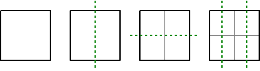
We partition the domain into hyperboxes, which we call blocks. Let be the unique positive integer such that As in the one-dimensional case, the final block covers the entire domain, i.e., . To construct the partition of , we apply the split procedure from Algorithm 2 to . Each split doubles the number of blocks, so after splits, consists of blocks. The splits proceed cyclically over the dimensions: the first along the first dimension, the second along the second, and so forth. After splits, we return to the first dimension and continue this process until all splits have been performed.
Elementary Blocks.
We refer to the blocks at the lowest level of our hierarchy as elementary blocks. Within an elementary block, all points are treated identically by Algorithm 1: by construction, the algorithm’s decisions do not depend on which specific point from the block is presented. Consequently, we may assume that the points drawn within an elementary block are i.i.d. samples from the uniform distribution 222Note that is the restriction of the global distribution to block ..
Block order.
At this stage, we impose an order on the blocks. Consecutive blocks are assigned to consecutive buckets/sub-subarrays. In addition, they are constructed so that they merge early during the execution of our algorithm. This motivates a further property: consecutive blocks must be neighbours, i.e., they share a face (or, more generally, a hyperface). We present Algorithm 3, which traverses the blocks in such an order, and establish its correctness in Lemma 14 which is formally proven in the Appendix of the full version.
Lemma 14.
Algorithm 3 visits every block exactly once, and any two consecutive blocks in the order are adjacent.
4.2 InBucketPlacement
Once mapped to a bucket, an element is placed in an empty cell using Bertram’s adversarial algorithm [6].
4.3 Cost Analysis
Similarly to the stochastic online sorting case, we distinguish three sources of cost: the intra-bucket cost, the inter-bucket cost, and the cost of connecting different subarrays. Since absolute values are not informative, all bounds will be expressed in terms of Opt. Before estimating Opt and analyzing each cost source separately, we recall several key results that will be used throughout the analysis.
Theorem 15 ([5]).
Given sufficiently large , the expected length of a TSP tour with points drawn i.i.d. from is , where . We denote this quantity by .
Corollary 16.
Since Opt represents the length of the optimal tour of points drawn i.i.d. from it is where the randomness is over the drawn instance.
Proposition 17.
The following properties hold:
-
1.
For all and all , we have .
-
2.
For any convex , let denote the expected length of the optimal TSP tour on points drawn uniformly i.i.d. in . Then,
Lemma 18 (Chapter 2, [15]).
Let be the length of the TSP of points drawn i.i.d. in . It holds for some constant :
Estimating the Optimal Cost.
In contrast to the one-dimensional case, there is no simple closed-form expression for the optimal cost in higher dimensions. We therefore rely on asymptotic estimates and concentration bounds to control the value of Opt.
Lemma 19.
With probability at least , the optimal TSP tour satisfies
We now proceed to the analysis of the three sources of cost.
Intra-Bucket Cost.
Lemma 20.
Let be the length of the optimal tour of points drawn uniformly at random from elementary block . Then,
Proof.
Step 1: Block side length.
Since the domain is split times, each dimension is split at least times333We assume that . In the full version we remove this assumption., thus the maximum side length of a block is at most . As and are integers, Hence, each side of has length at most .
Step 2: Expected cost.
The expected length of the optimal subtour inside satisfies:
where is the side length of . Substituting gives:
Step 3: Concentration.
Applying Lemma 18 with , we bound the probability that exceeds three times its expectation:
Corollary 21.
With probability at least , every one of the elementary block tours has length at most
So far, we proved that the length of the optimal tour of points uniformly chosen in a block is bounded by with probability at least . We want to transition from this to a bound of the optimal total intra bucket cost of a subarray , denoted by . For the first subarray, elementary blocks are mapped one to one to buckets and every bucket contains strictly less than points therefore Corollary 21 implies that with probability at least . We now show that any subsequent (fixed) subarray enjoys a comparable bound.
Lemma 22.
Fix an arbitrary phase and an arbitrary block of phase . Block consists of some elementary blocks . Fix any realization of points and let denoted the realized points inside block ,
where denotes the length of the optimal tour of the points in set .
Proof.
A feasible tour inside is obtained by concatenating the optimal tours of and adding at most connecting edges between adjacent elementary blocks. Summed over all phase blocks, the total number of such connectors is at most the number of elementary blocks. By Lemma 28, each connector has length at most , and by Corollary 30 the total intra-subarray connection cost is deterministically bounded by . This yields the claimed inequality.
At this point we restate Lemma 4 slightly changing the phrasing to fit current context.
Lemma 23.
For every subarray , each bucket has capacity less than points.
Corollary 24.
Each subarray gets at most points from any elementary block.
Lemma 25.
For any and any subarray , it holds .
Proof.
The cardinality of is a random variable. However, by Corollary 24, contains fewer than points. In both cases, the points are independently drawn uniformly at random within the same block. The proof then follows from the observation that the probability of the optimal tour length of i.i.d. points in some space exceeding a threshold is non-decreasing in the number of points .
Proposition 26.
Fix any subarray . With probability at least , it is .
Proof.
Lemma 25 combined with Lemma 20 implies . Taking a union bound over different elementary blocks and adding the connecting term completes the proof.
Corollary 27.
By taking a union bound over the subarrays we get that, with probability at least , for every subarray it holds .
Inter-Bucket Cost.
Lemma 28.
The cost of connecting two neighbouring blocks is at most
Remark 29.
Lemma 28 applies to elementary blocks. When moving to higher phases, blocks are formed by merging pairs of blocks from the previous phase. As a result, the diameter of a block (and hence the cost of connecting two neighboring blocks) increases by at most a factor strictly smaller than from one phase to the next. However, at the same time, the number of blocks to be connected decreases by a factor of at each phase. Therefore, the total cost incurred by connecting all blocks within a subarray remains of the same order, which leads to Corollary 30.
Corollary 30.
Using the observation above, the cost of connecting all blocks within a subarray is deterministically bounded by .
Cost of Connecting Subarrays.
Lemma 31.
The cost of connecting two subarrays is at most Opt.
Proof.
Connecting subarrays requires adding a single edge between two points, one from each subarray. Since the optimal tour Opt already spans all points in the domain, the additional cost of this connection is trivially bounded above by Opt.
Putting Everything Together.
We are now ready to prove Theorem 2. We decompose the total cost into four components:
-
Between subarrays: Connecting consecutive subarrays requires at most one additional edge per transition. By Lemma 31, this incurs cost at most Opt per transition. With subarrays, the total cost is .
-
Subarray : The remaining elements are placed in using Bertram’s algorithm [6], incurring total cost , since .
Conditioning on the high-probability event that Corollary 21 holds for all subarrays and conditioning on the event that the algorithm does not fail, the total cost of the algorithm is . This completes the proof of Theorem 2.
5 Conclusion and Open Directions
In this work, we study the stochastic variants of Online Sorting and Online TSP, obtaining polylogarithmic upper bounds in both settings. Analyzing the problem through the lens of the balls-into-bins paradigm reveals exponential improvements over previous approaches. A natural direction is to extend our bounds to general known distributions in higher dimensions. At the same time, our framework also assumes full knowledge of the distribution. Relaxing this assumption prompts several questions: What guarantees are possible when points are drawn i.i.d. from an unknown distribution, or when inputs arrive in uniformly random order with no distributional assumptions?
References
- [1] Anders Aamand, Mikkel Abrahamsen, Lorenzo Beretta, and Linda Kleist. Online Sorting and Translational Packing of Convex Polygons. In Nikhil Bansal and Viswanath Nagarajan, editors, Proceedings of the 2023 ACM-SIAM Symposium on Discrete Algorithms, SODA 2023, Florence, Italy, January 22-25, 2023, pages 1806–1833. SIAM, 2023. doi:10.1137/1.9781611977554.CH69.
- [2] Mikkel Abrahamsen, Ioana O. Bercea, Lorenzo Beretta, Jonas Klausen, and László Kozma. Online Sorting and Online TSP: Randomized, Stochastic, and High-Dimensional. In Timothy M. Chan, Johannes Fischer, John Iacono, and Grzegorz Herman, editors, 32nd Annual European Symposium on Algorithms, ESA 2024, September 2-4, 2024, Royal Holloway, London, United Kingdom, volume 308 of LIPIcs, pages 5:1–5:15. Schloss Dagstuhl – Leibniz-Zentrum für Informatik, 2024. doi:10.4230/LIPIcs.ESA.2024.5.
- [3] Giorgio Ausiello, Esteban Feuerstein, Stefano Leonardi, Leen Stougie, and Maurizio Talamo. Algorithms for the on-line travelling salesman, August 1999.
- [4] Yossi Azar, Debmalya Panigrahi, and Or Vardi. Nearly tight bounds for the online sorting problem, 2025. doi:10.48550/arXiv.2508.14287.
- [5] Jillian Beardwood, J. H. Halton, and J. M. Hammersley. The shortest path through many points. Mathematical Proceedings of the Cambridge Philosophical Society, 55(4):299–327, 1959. doi:10.1017/S0305004100034095.
- [6] Christian Bertram. Online Metric TSP, 2025. doi:10.48550/arXiv.2504.17716.
- [7] Dimitris Bertsimas and Michelangelo Grigni. Worst-case examples for the spacefilling curve heuristic for the euclidean traveling salesman problem. Operations Research Letters, 8(5):241–244, 1989. doi:10.1016/0167-6377(89)90047-3.
- [8] George Christodoulou and Alkmini Sgouritsa. An improved upper bound for the universal TSP on the grid. In Philip N. Klein, editor, Proceedings of the Twenty-Eighth Annual ACM-SIAM Symposium on Discrete Algorithms, SODA 2017, Barcelona, Spain, Hotel Porta Fira, January 16-19, pages 1006–1021. SIAM, 2017. doi:10.1137/1.9781611974782.64.
- [9] Dimitris Fotakis, Rasmus Pagh, Peter Sanders, and Paul Spirakis. Space efficient hash tables with worst case constant access time. In STACS 2003, 20th Annual Symposium on Theoretical Aspects of Computer Science, Berlin, Germany, February 27 - March 1, 2003, Proceedings, pages 271–282, February 2003. doi:10.1007/3-540-36494-3_25.
- [10] Mohammad T. Hajiaghayi, Robert Kleinberg, and Tom Leighton. Improved lower and upper bounds for universal tsp in planar metrics. In Proceedings of the Seventeenth Annual ACM-SIAM Symposium on Discrete Algorithm, SODA ’06, pages 649–658, USA, 2006. Society for Industrial and Applied Mathematics.
- [11] Yang Hu. Nearly optimal bounds for stochastic online sorting, 2025. doi:10.48550/arXiv.2508.07823.
- [12] William Kuszmaul. Fast concurrent cuckoo kick-out eviction schemes for high-density tables, 2016. arXiv:1605.05236.
- [13] Jubayer Nirjhor and Nicole Wein. Improved online sorting, 2025. doi:10.48550/arXiv.2508.14361.
- [14] Loren K. Platzman and John J. Bartholdi. Spacefilling curves and the planar travelling salesman problem. J. ACM, 36(4):719–737, 1989. doi:10.1145/76359.76361.
- [15] J. Michael Steele. Probability Theory and Combinatorial Optimization. Society for Industrial and Applied Mathematics, 1997. doi:10.1137/1.9781611970029.