An Almost-Optimal Upper Bound on the Push Number of the Torus Puzzle

Abstract
We study the Torus Puzzle, a solitaire game in which the elements of an input matrix need to be rearranged into a target configuration via a sequence of unit rotations (i.e., circular shifts) of rows and/or columns.
Amano et al. proposed a more permissive variant of the above puzzle, where each row and column rotation can shift the involved elements by any amount of positions. The number of rotations needed to solve the original and the permissive variants of the puzzle are respectively known as the push number and the drag number, where the latter is always smaller than or equal to the former and admits an existential lower bound of . While this lower bound is matched by an upper bound, the push number is not so well understood. Indeed, to the best of our knowledge, only an upper bound is currently known.
In this paper, we provide an algorithm that solves the Torus Puzzle using unit rotations in a model that is more restricted than that of the original puzzle. This implies a corresponding upper bound on the push number and reduces the gap between the known upper and lower bounds from to .
Keywords and phrases:
Torus puzzle, Push number, Permutation puzzlesCopyright and License:
![[Uncaptioned image]](x1.png) © Matteo Caporrella and Stefano Leucci; licensed under Creative Commons License CC-BY 4.0
© Matteo Caporrella and Stefano Leucci; licensed under Creative Commons License CC-BY 4.0
2012 ACM Subject Classification:
Mathematics of computing Permutations and combinations ; Theory of computation Design and analysis of algorithmsEditor:
John IaconoSeries and Publisher:
 Leibniz International Proceedings in Informatics, Schloss Dagstuhl – Leibniz-Zentrum für Informatik
1 Introduction
The Torus Puzzle, also known as Sliders, TwoBik, RotSquare, Loopover, or Sixteen Puzzle, is a solitaire game played on an matrix whose entries consist of (all and only) the integers from to . These elements are initially scrambled, and the goal is that of rearranging them via a sequence of unit rotations of rows and/or columns that causes the resulting arrangement of the elements to end up in the sorted configuration, i.e., in increasing order when read from left to right and from top to bottom.111More formally, the element on row and column of the sorted configuration is the integer . More precisely, a unit rotation of a row is specified by the row index and by a direction, which can be either leftward or rightward, and consists of a circular shift of all the elements in the chosen row along the chosen direction. Similarly, a column can be rotated either upward or downward. Figure 1 shows an example of such rotations.
It turns out that not all input matrices are sortable, and it is not hard to derive a characterization of sortable matrices which also serves as a linear-time algorithmic test (see the related works section for a more detailed discussion). This motivated previous research to consider only sortable puzzles and to provide general upper and lower bounds on the number of unit rotations needed to solve the puzzle. This quantity is known as the push number and was introduced by Amano et al. [2] along with the related notion of drag number, which counts multiple consecutive rotations of the same row or column only once. Equivalently, the drag number can be interpreted as the number of moves needed to solve the Torus Puzzle when each move allows rotating a row or column of choice by an arbitrary amount.222To be pedantic, [2] only defined the push and drag numbers for a specific sequence of rotations, and then introduced two functions and corresponding to the minimum push and drag numbers among all sequences of rotations that sort the elements of , respectively. We find it natural to refer to and as the push and drag numbers of instance , respectively.
Amano et al. showed a constructive upper bound of on the drag number of any sortable instance of the Torus Puzzle, along with a matching existential lower bound of , i.e., that there exists a constant such that, for any choice of and with , some sortable instance has a drag number of at least . Clearly, the push number is no smaller than the drag number, and it can never exceed it by more than a multiplicative factor of (since a rotation by an arbitrary amount can always be simulated using multiple unit rotations along the “shortest” direction).
Unfortunately, to the best of our knowledge, the best asymptotic lower and upper bounds on the push number, in terms of and , are exactly those obtained by combining the and bounds on the drag number given in [2] with the relations above. That is, there exists an algorithm that solves the Torus Puzzle using unit rotations, and any such algorithm needs to perform at least rotations in the worst case, leaving a multiplicative gap of between the upper and the lower bound.
Our results and techniques.
In this paper we make progress towards closing this gap by providing an algorithm solving any sortable instance of the Torus Puzzle using unit rotations, which is optimal up to polylogarithmic factors in the worst case. We also show that such a sequence of rotations can be found in the same asymptotic worst-case time. The above results hold in the even more restricted model in which the rotation directions cannot be freely chosen by the algorithm, but are independently specified, for each row and column, as part of the input instance.
While the solution strategy of [2] is based on repeatedly swapping triples of distinct elements, an operation that requires unit rotations, our algorithm follows a different approach which relies on three main ingredients. First, we treat all integers that should end up in the first row of the sorted configuration as some sort of buffer elements, whose exact positions can be (temporarily) disregarded; we move each remaining element to its intended final column, and the buffer elements to the first row. Next, we sort the non-buffer elements within each column using a strategy akin to that of RadixSort. This requires handling multiple columns in parallel in order to meet the claimed upper bound on the number of moves. Finally, we deal with the buffer elements: since they are all on the first row, the challenge is that of suitably permuting them without affecting the placement of the other elements. As an intermediate step, we show how to simultaneously swap a collection of pairwise-disjoint pairs of buffer elements while causing only controlled side effects to the rest of the matrix. We can then combine multiple parallel swaps in a way that ensures that their side effects cancel out, thus obtaining the sought sorted matrix.
Some historic notes and related works.
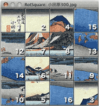
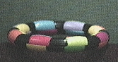
The earliest report we found of the Torus Puzzle dates back to 1981, when Takeshi Ogihara implemented it on a Mitsubishi MELCOM mainframe using a text-based interface. In 1993, following Ogihara’s suggestion while he was involved in upgrading Osaka University’s mainframes to NeXT computers, M. Torigoe, a Faculty of Science student, reimplemented the puzzle as a graphical NeXTSTEP application named RotSquare. Ogihara later ported RotSquare to OpenStep, Mac OS X, and iOS (see Figure 2 (left) for a screenshot) [23]. Several successive implementations have been independently produced under various names. A commercial physical realization of a puzzle that appears very similar to a Torus puzzle has been reported to exist back in 1987 on the MIT’s CubeLovers mailing list (see [25, 19, 18] and Figure 2 (right) for a 1995 photo). Another puzzle involving a toroidal movement mechanic is implemented by the 1992 video game Yoshi’s Cookie for the Nintendo Entertainment System, where players must rotate rows and columns of a grid in order to match similar elements à la Bejeweled [17, 14].
The first mention of the Torus Puzzle in a mathematical context was in 1988, when Diaconis considered the version as an easier to analyze variant of the Fifteen Puzzle, showing that random rotations are enough to randomize the position of each individual element and conjecturing that rotations suffice to shuffle all elements [10, p. 90]. Diaconis’ conjecture is still open to this day, and the best-known upper bound for the Torus Shuffle is of random rotations [5].
In 1997, mathematician Alexander Bogomolny [6] described the puzzle on his website under the name Sliders Puzzle. He proved that every matrix is sortable by providing an explicit strategy that swaps two elements of choice without affecting the positions of the other elements. In general, each arrangement of the elements of an matrix can be seen as a permutation of , with the sorted configuration corresponding to the identity permutation. Bogomolny observed that, in any puzzle with odd , all rotations correspond to even permutations, hence all configurations reachable from the initial one must have its same parity. Moreover, all such parity-preserving configurations can actually be reached when is odd. For even values of , the elements can always be rearranged into any configuration of choice. Bogomolny’s impossibility argument immediately extends to rectangular matrices: an matrix in which both and are odd is sortable only if the permutation induced by the initial configuration of the elements is even.
In 1999, Donald Lee Greenwell gave explicit sequences swapping any two adjacent elements in and matrices [13], and argued that similar swaps can be performed in any matrix, as long as at least one of and is even. Greenwell also proposed two additional variants of the puzzle, where rows and columns wrap around as if they were laid out on a Klein bottle or on the projective plane.
Later, Amano et al. [2] considered general matrices and described a sequence of rotations performing a three-element swap: given three distinct elements , it is possible to move each to the position of without affecting the placement of the other elements.
Then, the authors show how a sequence of three-element swaps can sort any matrix where at least one of , , and the initial permutation of the elements is even.
Since each three-element swap can be implemented by a sequence consisting of a constant number of compound rotations333We use compound rotation to refer to multiple consecutive unit rotations of the same row or column. of rows and columns,
this implies an upper bound of on the drag number. However, the overall number of unit rotations required by a three-element swap can be as large as , yielding the best-known upper bound of on the push number.
As observed by [2], a lower bound on the drag number (and on the push number) can be obtained by noticing that there are at least distinct sortable matrices
and at most distinct sequences of up to (possibly compound) rotations, implying that some sortable matrix requires at least rotations to be sorted.
To summarize, the results in [6, 13, 2] characterize the sortable instances of the Torus Puzzle:
Remark 1.
An instance of the Torus Puzzle can be sorted through a sequence of row and column rotations if and only if at least one of , , and the permutation of induced by the arrangement of elements in is even.
Several heuristic strategies for finding solutions to Torus Puzzle instances have been proposed in [15], and a colored variant of the Torus Puzzle has been shown to be -Hard in [2]. In this variant, each entry of the matrix consists of one of two colors, and the goal is that of determining whether some target arrangement of colors can be reached.
The Torus Puzzle falls into the general category of permutation puzzles [11, 21]: the input configuration is an element of a suitable permutation group, and the goal is that of deciding whether it belongs to the same connected component of the desired target configuration. If the answer is affirmative, then one can also look for a sequence of moves transforming the initial configuration into the target one, or even for the shortest such sequence. These two problems correspond to the generalized word problem and to the shortest word problem on the associated permutation group. Some other notable puzzles in this category are the Fifteen Puzzle [3, 24, 9, 12], the Rubik’s Cube [7, 8] including a variant played on a torus [1], several other swapping token problems (see, e.g., [20, 4, 16, 26] and the references therein), and rotating puzzles on graphs [27, 22]. In particular, the latter appear to be close in spirit to the Torus Puzzle: given a graph with an element on each vertex, the goal is that of rearranging these elements into a target configuration via a sequence of rotations along the cycles of . An instance of the Torus Puzzle can be seen as a rotating puzzle on an torus graph, with the further restriction that only some of the cycles can be rotated.
Finally, we mention that the problem of finding lower and upper bounds to the drag and/or push numbers of Torus Puzzle can be cast as the problem of finding corresponding bounds on the diameter of the Cayley graph of the associated permutation group.
Organization of the paper.
Section 2 introduces the notation used throughout the paper and recalls some standard definitions. Section 3 presents our sorting algorithm, which solves any sortable instance of the Torus puzzle using unit rotations. For the sake of simplicity, we assume that the allowed (unit) row rotations are all in the rightward direction, while columns can only be rotated downward. Section 4 discusses how the algorithm can be implemented to run in time , how it can be adapted to handle the case in which each row and column can only be rotated in a direction specified as part of the input, and the problems left open.
A playable version of the puzzle, along with an implementation of our algorithm, is available at https://www.isnphard.com/g/torus-puzzle/, which might help the reader visualize the different subroutines discussed in the technical part of the paper.
2 Preliminaries
Matrices and rotations.
We use to refer to the matrix to be sorted, and we assume that .444Given an or a matrix , it is easy to design a linear-time algorithm deciding whether can be sorted and, if that is the case, returning a sequence of moves that sorts . For an integer , we denote by and the target row and the target column in which should be placed in the sorted configuration, respectively, i.e., we let and , where rows and columns are numbered from .
The first row of will be denoted by , while will denote either the position on the -th column of or the element contained therein, depending on context. Similarly, the -th column of will be denoted by , and the element or position on the -th row of will be denoted by . We refer to and as the head and the tail of , respectively. The body of refers to all positions/elements that are in column but not in ’s head (notice that the tail of a column is part of its body). Observe that contains all and only the columns’ heads and, more precisely, coincides with .
Since the model considered in the next section only allows for unit rightward rotations of rows, and unit downward rotations of columns, we refer to a row/column notation by the name of the corresponding row/column, and we may omit the terms “unit”, “rightward”, or “downward”. A non-negative integer superscript denotes consecutive rotations of the same row/column, and we may write a sequence of rotations involving multiple rows/columns by juxtaposing row and column names with their respective superscripts. Sequences are evaluated from left to right. For example, is equivalent to and denotes three consecutive downward rotations of , followed by two rightward rotations of , followed by a downward rotation of .
If and are two positions in the matrix, and is a sequence of rotations, we write to denote that, as a result of applying the sequence , the element initially placed in ends up in position . If are positions and are sequences of rotations such that , we might express this compactly using the shorthand . Observe that the above implies , where denotes the concatenation of , in this order.
Permutations.
Since each rotation can also be interpreted as permutation of the elements in , we employ the left-to-right convention for permutation products. In this way, the configuration of elements resulting from a sequence of rotations corresponds to the action on of the permutation resulting from their product. Finally, we briefly recall some standard concepts used in the paper: a permutation can be decomposed into a product of some number of disjoint cycles555A cycle of length is a permutation such that: (i) all elements are distinct, (ii) for , (iii) , and (iv) for all . , i.e., . A transposition is a permutation consisting of a single cycle of length , and an involution is a permutation in which each cycle has length at most , i.e., each cycle is either a fixed-point (a cycle of length ) or a transposition. The number of cycles of length of a permutation is denoted by . Each permutation can be written as either a product of an even number of transpositions, or as a product of an odd number of transpositions, but not both, and the parity of is defined as the parity of the number of such transpositions. If a permutation of elements has cycles (including its fixed-points), then the parity of is equal to the parity of . Moreover, the parity of a permutation is the same as that of its inverse . The product of two permutations and is even if and only if the parities of and are the same (i.e., and are both even or both odd).
3 Solving the Torus Puzzle using unit rotations
In this section we provide an algorithm solving any sortable instance of the Torus Puzzle using only rotations. We consider the case in which all rows can only rotate rightward while columns can only rotate downward. In Section 4 we discuss how arbitrary rotation directions can be handled.
We start with some definitions. We say that a column is near-full if all elements in the body of satisfy , i.e., they are in their target column. If is not near-full, we say that it is underfull. A column is body-full if it is near-full and its body contains all (and only) the elements with and . In other words, the body of contains exactly the same set of elements as that in the sorted configuration, but these elements can appear in an arbitrary order. Finally, a column is body-sorted if all elements in its body are in their respective target positions.
The algorithm first makes all columns near-full, then body-full, then sorts their bodies in groups so that all columns become body-sorted, and finally handles sorting the first row. Each of the following subsections describes one of the above steps, in the above order.
3.1 Making columns near-full
We start by describing a procedure, which we name FillColumns, that receives as input an matrix with and rearranges the elements in via a sequence of rotations to ensure that all columns of the resulting configuration are near-full. Intuitively, the algorithm uses the first row as a sort of “sushi belt” from which each column can “pick up” a desirable element while simultaneously “discarding” an undesirable one.
In details, is repeatedly rotated and, whenever (i) some element in ends up in its target column (i.e., ), and (ii) such a column is underfull, then is also rotated.
The rotation of causes to move from the head to the body of , and the tail of to move to the head of (in place of ), i.e., and .
These column rotations are repeated until either becomes near-full, or the target column of the new head of is no longer (possibly both).
When no element in satisfies conditions (i) and (ii), the procedure resumes rotating the first row. The procedure stops as soon as all columns are near-full. The pseudocode of FillColumns is shown in Algorithm 1, while Figure 3 shows a possible input, an intermediate configuration, and the resulting output.
We start our analysis by bounding the number of column rotations.
Lemma 2.
The number of column rotations performed by FillColumns is .
Proof.
We prove the claim by focusing on a generic column and showing that, once is rotated times, FillColumns performs no additional rotations on .
Indeed, FillColumns ensures that each rotation of moves some element having target column into the body of and, specifically, into . Since additional downward rotations of are needed for to leave the body of , we have that after performing any number rotations of , the body of contains at least elements whose target column is . Then, if the -th rotation of is performed, it must result in a column that is near-full. The claim follows by observing that FillColumns only rotates columns that are not near-full.
Let be the input matrix to FillColumns, and let be the matrix as arranged immediately after the completion of the -th iteration of the outer while loop of Algorithm 1, if it exists. We associate a potential to each , where is defined as the number of elements in that are in the body of some column other than their target column, i.e., . The following lemma shows that each group of iterations of the outer while loop starting from some configuration decreases the potential by at least half the number of underfull columns in .
Lemma 3.
Consider a configuration with underfull columns. If exists, then .
Proof.
We assume that exists since otherwise the claim is trivially true. For an underfull column of , we let be the set of elements in that have as their target column (i.e., such that ), while for each near-full column we let .
Since row of configuration contains at most one element with target column for each of the near-full columns , there must be at least distinct elements in whose target column is underfull. Hence, .
In the rest of the proof we argue that at least elements from are placed in the bodies of their respective columns in . Since the only way for FillColumns to move an element from the head to the body of its target column is that of rotating until some other element with ends up in , causing to decrease by , this will imply that , as claimed.
In particular, we focus on a specific column with , and we show that at least of the elements in are in the body of in configuration . Since row is rotated times from configuration to configuration , and is only rotated if , we have that each element becomes the head of in some (distinct) configuration with . Let be the elements in , in increasing order of . Consider then the -th iteration of the outer while loop of FillColumns. If or , then is underfull in , which means that is moved to the body of in such iteration, and never leaves it in the following iterations. It follows that at least elements are in the body of in configuration .
The above lemma allows us to upper bound the number of rotations of the first row.
Lemma 4.
The number of rotations of performed by FillColumns is .
Proof.
We partition the rotations of performed by FillColumns into phases. We say that a configuration belongs to the -th phase if its number of underfull columns lies in the half-open interval . We also say that a rotation of belongs to phase if the configuration from which it is performed belongs to phase .
By our definition of , we have that if is in phase , then . Moreover, Lemma 3 ensures that, if exists, then . This shows that there can be at most disjoint groups of rotations of in phase . Hence, the number of rotations of in each phase is at most . The claim follows by multiplying by the number of phases.
The stopping condition of FillColumns, together with Lemma 2 and Lemma 4, imply the following corollary, which summarizes the result of this section.
Corollary 5.
Given an input matrix with , FillColumns performs rotations and rearranges the elements in so that all columns become near-full.
3.2 Transforming near-full columns into body-full columns
Once all the columns of a configuration are near-full, it is easy to see that rotations suffice to rearrange the elements in so that all columns become body-full. This is exactly the purpose of our next procedure, which we name FloatMinimums. The corresponding pseudocode is given in Algorithm 2, while Figure 4 shows an example input configuration along with the resulting output.
We start by noticing that the fact that all columns of are near-full implies that contains exactly one element with per column . FloatMinimums uses this fact by performing rotations of : before each rotation, it checks whether any element in is on its target column . Whenever this is the case, column contains all (and only) the elements having as their target column (in some arbitrary order), and FloatMinimums rotates until its head becomes the unique element with and , thus making body-full with at most rotations of . Column will never be rotated again by the procedure. Hence, we have the following:
Lemma 6.
Given an input matrix in which all columns are near-full, procedure FloatMinimums performs rotations and rearranges the elements in so that all columns become body-full.
3.3 Transforming body-full columns into body-sorted columns
In this section, we show how a configuration of an matrix , with , in which all columns are body-full, can be transformed into a configuration in which all columns are body-sorted using rotations.
Sorting the body of a single column.
As a warm-up, we start by sketching how a single body-full column can be made body-sorted using rotations. The procedure will only rotate and , hence all elements in the body of columns other than will remain in their initial positions. In particular, any other column that is already body-full (resp. body-sorted) will remain body-full (resp. body-sorted). This also means that the set of elements in will remain unchanged, although their order might change.
The idea is that of simulating the RadixSort algorithm on the elements in the body of . We achieve this by repeatedly unloading the body of into and then re-loading the same elements back into in a suitable order. In particular, the procedure consists of phases, where the -th phase sorts the elements of according to the -th least significant bit of (a suitably shifted version of) . This sorting step is stable; hence, after the last phase is completed, column is body-sorted.
In details, a phase is subdivided into three sub-phases. In the first sub-phase we unload all elements of into with the sequence of rotations , which also ensures that the overall number of rotations of is . The second sub-phase rotates additional times and, before each rotation, we check whether the element on the head of should be moved to the body of , namely if , , and the -th least significant bit of is set. At this point, has been rotated times, and all the elements that were originally in the body of and have their -th least significant bit set are now in the body of . The third and final sub-phase is similar to the second one, with the only difference that the condition is replaced with . This loads the remaining elements into . Observe that in the second and third sub-phases, the elements inserted in are encountered in the same order in which they were unloaded, hence each phase is stable.
Unfortunately, while sequentially applying the above simulation of RadixSort on each column would render all columns body-full, this would require rotations, which is asymptotically larger than our goal whenever .
Sorting the bodies of up to columns.
To circumvent this issue, we show how to generalize the above RadixSort-inspired scheme to handle a number of up to columns in parallel. The resulting procedure, which we name RadixSortBodies, performs rotations and its pseudocode is given in Algorithm 3.
Let be a set of column indices. RadixSortBodies starts by unloading, in parallel, the bodies of all columns with into . In order to do that, we choose pairwise-disjoint subsets of , each containing elements, e.g., we can choose .666The algorithm described previously for sorting the body of a single column corresponds to the case , , and the choice (where the second set of the union might be empty). Intuitively, set is associated to column and contains the indices corresponding to the positions into which RadixSortBodies unloads the elements in the body of .
As before, the procedure works in phases, where the -th phases is concerned with sorting the elements of interest w.r.t. their -th least significant bit. Similarly, each phase is also split into three sub-phases.
The first sub-phase unloads all elements in the body of the columns with into . In order to do so, we define so that, as a result of performing rotations of , the element that ends up in is the one that was originally placed in . In this sub-phase, row is rotated times and, before each rotation, we check whether for each . For all that satisfy the above condition, we rotate , thus moving the element currently on the tail of into .
The second and third sub-phases behave similarly to one another, and handle the elements having their -th least significant bit set to and , respectively. The second (resp. third) sub-phase, rotates times and, before each rotation, checks whether any of the elements currently on the heads the columns whose bodies are to be sorted should be loaded into their column’s body. More precisely, if is the head of some column with , this happens when , , and for the second sub-phase (resp. for the third sub-phase). Notice that, within each of the last two sub-phases, the loaded elements are inserted in the bodies of the respective columns in the same order as they were unloaded in the first phase, hence the overall algorithm is stable. Figure 5 shows some configurations encountered during an execution of RadixSortBodies.
Sorting all column bodies.
It is now easy to transform any matrix in which each column is body-full into a matrix in which each column is body-sorted using rotations.
Indeed, it suffices to arbitrarily partition the columns into groups of columns each, except possibly for (which has size ).
Then, we iteratively make the columns in each group body-full by invoking RadixSortBodies on the columns in , which requires rotations.
Since the number of groups is , the overall number of rotations is .
The following lemma summarizes the discussion in this section.
Lemma 7.
Given an input matrix with and in which all columns are body-full, there exists a procedure that performs rotations and rearranges the elements in so that all columns become body-sorted.
3.4 Sorting the first row
We now have a sortable matrix where all columns are body-sorted, which implies that contains all and only the elements with , and we are left with the task of sorting the elements in . In particular, the arrangement of elements in can be interpreted as that resulting from the action of some permutation on the set . Then, our goal becomes that of finding a sequence of row and column rotations whose net result is that of applying to . This turns out to be more or less challenging depending on the parity of and on that of .777The elements of , in order, coincide with those of the one-line representation of .
In the rest of this section we build up towards this goal by first showing a way to apply an involution to while keeping side effects under control, and then using such result to handle general permutations.
Swapping pairs of elements in .
We start by describing an auxiliary procedure that takes as input a collection of pairs of column indices, where all such indices are distinct, and swaps each element in with that in , for all . We name this procedure SwapPairs and we give its pseudocode in Algorithm 4.
SwapPairsperforms rotations but produces some side effects. More precisely, the procedure needs to use a distinct auxiliary column for each pair which, for the sake of simplicity, we chose to be column . The elements in the body of each auxiliary column will undergo a circular shift, which can be either upward (i.e., moves to for , and moves to ) or downward (i.e., moves to for , and moves to ). The direction of these rotations is controlled by an additional input parameter , where U (resp. D) denotes an upward (resp. downward) rotation.
We note that these side effects are unavoidable as long as the algorithm needs to work for matrices of arbitrary dimensions. Indeed, it is impossible to swap two (or any even number of pairs of) elements without introducing side effects, as this would allow one to change the parity of the permutation induced by positions of the elements in the matrix (see Remark 1).
The procedure works in three phases. In the first phase, row is rotated times. Before the generic -th rotation, we check for which indices the element originally in is now in , i.e., i.e., we check whether . For any such index , we rotate one time if or times if (effectively simulating an upward rotation of ). Denoting with the sequence of all rotation performed in the first phase, the overall effect of the phase is the following, where and all elements that not explicitly handled are unaffected:
-
When , , , and for ;
-
When , , , and for .
In the second phase, is again rotated times. Before the generic -th rotation, we find all columns that satisfy , and we rotate each such column times if , or one time if . The net effect of the sequence of rotations performed during the second phase (on the matrix resulting from the first phase) is the following:
-
When , , , and for .
-
When , , , and for ;
The third and final phase is identical to the first one, hence its sequence of rotations produces the same net effect (on the matrix resulting from the second phase) as that of sequence . Figure 6 shows some example configurations obtained after the different phases, and after successive executions of SwapPairs.
We can now use SwapPairs to apply any involution to , as the following lemma shows.
Lemma 8.
Consider an matrix . Given an involution on and , there exists a procedure that uses rotations and produces the following effects: (i) permutes according to , and (ii) if (resp. ) performs a cyclic upward (resp. downward) rotation of the body of each with .
Proof.
Let be the transpositions of , where . We invoke SwapPairs using the same value of as the one in the statement and with the pairs of column indices for .
We now prove that such a call has the desired effect. To see that each pair of elements with is indeed swapped, observe that:
-
When , and .
-
When , and .
To see that the body of each column with undergoes the claimed circular shift, observe that:
-
When , for , and .
-
When , for , and .
To conclude the proof, notice that all elements not explicitly discussed above retain their positions after the rotations in , , and .
Decomposing into involutions and transpositions.
We now employ the above result to place all elements in in their target position, while keeping all columns body sorted, and possibly causing circular shift in the body of .
It is folklore that any permutation can be written as the product of two involutions (see, e.g., [28]). One can also ensure that, when is even, these two involutions have the same number of transpositions, while the odd case requires one more transposition. We formally state this result in the following two lemmas, in a way that is convenient for the sequel.
Lemma 9.
Let be a permutation that consists of a single non-trivial cycle. If is even, then there exists two involutions , such that and . If is odd, then there exists four involutions , , , such that , , and .
Proof.
Assume w.l.o.g. that . The proof is split in two cases, depending on the parity of . If is even, then for some positive integer . We choose , and . Observe that . An example is shown in Figure 7 (left).
If is odd, then for some positive integer . We choose , and . Observe that and . An example is shown in Figure 7 (middle). We also choose and . Observe that and . An example is shown in Figure 7 (right).
Lemma 10.
Let be a permutation. If is even, then there exist two involutions such that , and . If is odd, then there exist two involutions and a transposition such that , and .
Proof.
Let and be the non-trivial even and odd cycles of , respectively. Lemma 9 shows that we can write each even cycle as , where and are two involutions with the same number of transpositions. We let and . Similarly, Lemma 9 shows that we can write each odd cycle as both and , where each of , , , and is an involution, , and .
The rest of the proof depends on the parity of . We consider the case in which is even first, which implies that is also even. We let and (notice the alternating superscripts). The claim follows by choosing and .
We now consider the case in which is odd, which implies that is also odd. We let be an arbitrary transposition of , and we define as the involution obtained by removing from (observe that is its own inverse), so that . We let and (notice the alternating superscripts). The claim follows by choosing , , and as defined above.
Applying to .
We can finally show how the elements in can be sorted, i.e., permuted according to . We start with a simplification: we assume w.l.o.g. that if is odd, then is even. Indeed, the case in which is odd and is odd can be avoided by noticing that, whenever this happens, must be even since otherwise the matrix would not be sortable (see Remark 1). Hence, we can reduce to the case in which is even by rotating .
We proceed differently depending on the parity of . If is even, we use Lemma 10 to write as the product of two involutions with . Then we execute procedure SwapPairs twice: the first call applies to and uses , while the second applies to the resulting configuration and uses . Invoking Lemma 8 twice shows that all rotations caused to the column bodies cancel out, while the elements originally in get permuted according to , i.e., they end up in the sorted configuration.
The only remaining case is the one in which is odd and is even. In this case, we use Lemma 10 to write as the product of two involutions with , and a transposition . We call procedure SwapPairs five times. The first two calls apply involutions and to , in this order, with and respectively. Using Lemma 8 twice, we have that the combined effect of these two calls to SwapPairs leaves the positions of the elements not in unaffected. The third call swaps the elements involved in the transposition , while causing a circular shift in body of (the direction of such shift is not important). Since is even, the number of elements in the body of is odd, and the permutation describing their circular shift is even, hence it can be written as the product of two involutions with the same number of transpositions. Since we can equivalently consider the transposed version of matrix , we use the fourth and fifth calls to SwapPairs to apply and , in this order, to the first row of , i.e., to column of . By using opposite values of in these two final calls, we ensure any side effects introduced by the fourth call are undone by the fifth and last call. An example is provided in Figure 8. The above discussion is summarized in the following lemma.
Lemma 11.
Given an matrix in which each column is body-sorted, there exists a procedure that performs rotations and sorts .
Algorithm 5 shows the final pseudocode for solving the Torus Puzzle when (which can be assumed w.l.o.g.), where lines from 6 onward handle sorting as described above.
The main result of this paper follows from combining Corollary 5 and Lemmas 6, 7, and 11.
Theorem 12.
There exists an algorithm that, given a sortable instance of the Torus Puzzle, sorts it by performing rotations, where each rotation is either a unit downward rotation of a column or unit rightward rotation of a row.
4 Concluding remarks and open problems
Remarks on the time-complexity of our algorithm.
An implementation of the procedures used in our algorithm which closely follows the provided pseudocodes can result in a running time that is larger than our upper bound on the push number.
Here, we briefly sketch how the algorithm can be implemented to also run in time . We start by observing that, when , the only row rotated by procedures FillColumns, FloatMinimums, RadixSortBodies, and SwapPairs is . Then, a data structure that maintains the current configuration of while allowing constant-time element access, and constant-time (not necessarily unit) rotations of and can be obtained by storing and each of the column bodies in circular arrays equipped with pointers to their first elements. Moreover, for a given column and at any point during the execution of FillColumns, FloatMinimums, each (sub-)phase of RadixSortBodies, and each of the three phases of SwapPairs, it is easy to know when the next rotation of will occur. The idea is that of introducing a concept of time, which is determined by the number of rotations of performed so far, while maintaining a min-heap storing each of column index with a key equal to the time of the next rotation of (if any). Since the next rotation of a column (if it exists) is never more than time-instants away, can be implemented to support insertions in constant-time, and extractions of the minimum in time proportional to the number of time-instants between the current time and the one given by the key of the extracted element. With these ingredients, all the above procedures can be implemented to run in the same asymptotic time as their respective upper bounds on the number of rotations, and the same follows for the whole sorting algorithm (which, for , repeatedly invokes these procedure while transposing at most once).
Reducing the number of distinct rotation types.
When our algorithm is executed on an input matrix with , all rotations involve or the columns up until the very end, when SwapPairs might be invoked to apply the permutation to (i.e., to the first row of the transposed version of ). This last step may rotate rows other than .
One might wonder whether it is possible to avoid rotating these rows, since doing so would result in an algorithm that sorts any sortable matrix using no more than distinct rotation types, which is also a lower bound.888To see that rotation types are not enough in general, notice that at least one row and at least one column must necessarily be available for rotations. Then, for any such choice of rotations types, there is always a row-column pair such that neither the row nor the column can be rotated, which implies that the element on their intersection cannot be moved from its initial position. This can be by using the following alternative handing of the case in which is odd (i.e., the “else” branch starting at line 13 of Algorithm 5): after decomposing into the product , call SwapPairs with alternating choices of to apply , , , and to , in this order. This results in a matrix in which every element is in its target position, except for and , which need to be swapped. In the full version of the paper, we show a sequence of unit rotation that performs exactly this task when is even (as in the case of interest), while only rotating and .
Handling arbitrary rotation directions.
While the description of our algorithm assumes that all columns can only be rotated downwards, it is easy to check that all our procedures work with either no or with minor modifications even when each column can only be rotated in a direction specified as part of the input (where different columns can have different directions). This implies that our upper bound holds even when both rows and columns have input-specified rotation directions. The easiest way to see this is that of combining the previous discussion showing that the only row that needs to be rotated is , with symmetry arguments which allow to equivalently consider a transposed or mirrored version of .999In this way, one can always assume to be dealing with a matrix with at least as many columns as rows, and where unit rightward rotations of the first row are allowed.
Open problems.
Following our results, the known lower and upper bounds on the push number differ by a multiplicative factor. It would be interesting to close this gap by providing asymptotically tight bounds.
Moreover, to the best of our knowledge, it is still unknown whether the optimization version of the Torus Puzzle (that asks to return the shortest sequence of rotations sorting the input matrix) is solvable in polynomial time, both for the case unit rotations and for the more permissive case of compound rotations. Likewise, no polynomial-time approximation algorithm with an approximation factor better than the trivial is currently known.
References
- [1] Jeremy F. Alm, Michael Gramelspacher, and Theodore Rice. Rubik’s on the torus. Am. Math. Mon., 120(2):150–160, 2013. doi:10.4169/AMER.MATH.MONTHLY.120.02.150.
- [2] Kazuyuki Amano, Yuta Kojima, Toshiya Kurabayashi, Keita Kurihara, Masahiro Nakamura, Ayaka Omi, Toshiyuki Tanaka, and Koichi Yamazaki. How to solve the torus puzzle. Algorithms, 5(1):18–29, 2012. doi:10.3390/A5010018.
- [3] Aaron F Archer. A modern treatment of the 15 puzzle. The American Mathematical Monthly, 106(9):793–799, 1999.
- [4] Davide Bilò, Maurizio Fiusco, Luciano Gualà, and Stefano Leucci. Swapping mixed-up beers to keep them cool. In Andrei Z. Broder and Tami Tamir, editors, 12th International Conference on Fun with Algorithms, FUN 2024, Island of La Maddalena, Sardinia, Italy, June 4-8, 2024, volume 291 of LIPIcs, pages 5:1–5:18. Schloss Dagstuhl – Leibniz-Zentrum für Informatik, 2024. doi:10.4230/LIPIcs.FUN.2024.5.
- [5] Olena Blumberg, Ben Morris, and Alto Senda. Mixing time of the torus shuffle. arXiv preprint arXiv:2411.06006, 2024.
- [6] Alex Bogomolny. Cut The Knot! — Slider Puzzles. Webpage, 1997. Accessed on 2025-12-29. URL: https://www.cut-the-knot.org/pythagoras/sliders.shtml.
- [7] Erik D. Demaine, Martin L. Demaine, Sarah Eisenstat, Anna Lubiw, and Andrew Winslow. Algorithms for Solving Rubik’s Cubes. In Camil Demetrescu and Magnús M. Halldórsson, editors, Algorithms - ESA 2011 - 19th Annual European Symposium, Saarbrücken, Germany, September 5-9, 2011. Proceedings, volume 6942 of Lecture Notes in Computer Science, pages 689–700. Springer, 2011. doi:10.1007/978-3-642-23719-5_58.
- [8] Erik D. Demaine, Sarah Eisenstat, and Mikhail Rudoy. Solving the Rubik’s Cube Optimally is NP-complete. In Rolf Niedermeier and Brigitte Vallée, editors, 35th Symposium on Theoretical Aspects of Computer Science, STACS 2018, Caen, France, February 28 - March 3, 2018, volume 96 of LIPIcs, pages 24:1–24:13. Schloss Dagstuhl – Leibniz-Zentrum für Informatik, 2018. doi:10.4230/LIPIcs.STACS.2018.24.
- [9] Erik D. Demaine and Mikhail Rudoy. A simple proof that the -puzzle is hard. Theor. Comput. Sci., 732:80–84, 2018. doi:10.1016/J.TCS.2018.04.031.
- [10] Persi Diaconis. Group representations in probability and statistics. Lecture notes-monograph series, 11:i–192, 1988.
- [11] Sebastian Egner and Markus Püschel. Solving puzzles related to permutation groups. In Volker Weispfenning and Barry M. Trager, editors, Proceedings of the 1998 International Symposium on Symbolic and Algebraic Computation, ISSAC ’98, Rostock, Germany, August 13-15, 1998, pages 186–193. ACM, 1998. doi:10.1145/281508.281611.
- [12] Oded Goldreich. Finding the shortest move-sequence in the graph-generalized 15-puzzle is np-hard. In Oded Goldreich, editor, Studies in Complexity and Cryptography. Miscellanea on the Interplay between Randomness and Computation, volume 6650 of Lecture Notes in Computer Science, pages 1–5. Springer, 2011. doi:10.1007/978-3-642-22670-0_1.
- [13] Donald Lee Greenwell. Cut The Knot! — Sliders, puzzles on graphs. Webpage, 1999. Accessed on 2025-12-29. URL: https://www.cut-the-knot.org/pythagoras/SLIDER.shtml.
- [14] Luciano Gualà, Stefano Leucci, and Emanuele Natale. Bejeweled, candy crush and other match-three games are (np-)hard. In 2014 IEEE Conference on Computational Intelligence and Games, CIG 2014, Dortmund, Germany, August 26-29, 2014, pages 1–8. IEEE, 2014. doi:10.1109/CIG.2014.6932866.
- [15] Colin Hemphill and Joshua Sheehy. Finding effective search strategies for the twobik puzzle. In Randy K. Smith and Susan V. Vrbsky, editors, Proceedings of the 50th Annual Southeast Regional Conference, 2012, Tuscaloosa, AL, USA, March 29-31, 2012, pages 53–58. ACM, 2012. doi:10.1145/2184512.2184526.
- [16] Sam Hiken and Nicole Wein. Improved hardness-of-approximation for token-swapping. In Anne Benoit, Haim Kaplan, Sebastian Wild, and Grzegorz Herman, editors, 33rd Annual European Symposium on Algorithms, ESA 2025, Warsaw, Poland, September 15-17, 2025, volume 351 of LIPIcs, pages 57:1–57:16. Schloss Dagstuhl – Leibniz-Zentrum für Informatik, 2025. doi:10.4230/LIPIcs.ESA.2025.57.
- [17] Jesper Juul. Swap adjacent gems to make sets of three: A history of matching tile games. Artifact: Journal of Design Practice, 1(4):205–217, 2007.
- [18] Andrew A. Kinsman. Re: Twist torus [small picture]. Message posted to the MIT’s CubeLovers mailing list, December 1995. Posted as “Andy Kinsman 66672”; Message ID: 9512151350.AA20112@newt.PCD1. URL: https://cube20.org/cubelovers/CL18/036.txt.
- [19] Serge Kornfeld. Re twist torus. Message posted to the MIT’s CubeLovers mailing list, December 1995. Message ID: 199512141816.NAA28270@spank.nexen.com. URL: https://cube20.org/cubelovers/CL18/031.txt.
- [20] Daniel Kornhauser, Gary L. Miller, and Paul G. Spirakis. Coordinating pebble motion on graphs, the diameter of permutation groups, and applications. In 25th Annual Symposium on Foundations of Computer Science, West Palm Beach, Florida, USA, 24-26 October 1984, pages 241–250. IEEE Computer Society, 1984. doi:10.1109/SFCS.1984.715921.
- [21] Jamie Mulholland. Permutation puzzles: a mathematical perspective. Departement Of mathematics Simon fraser University, 54, 2016.
- [22] Win Hlaing Hlaing Myint, Ryuhei Uehara, and Giovanni Viglietta. Token shifting on graphs. Int. J. Comput. Math. Comput. Syst. Theory, 7(4):223–234, 2022. doi:10.1080/23799927.2022.2118622.
- [23] Takeshi Ogihara. Personal communication, January 2026.
- [24] Daniel Ratner and Manfred K. Warmuth. Finding a shortest solution for the N × N extension of the 15-puzzle is intractable. In Tom Kehler, editor, Proceedings of the 5th National Conference on Artificial Intelligence. Philadelphia, PA, USA, August 11-15, 1986. Volume 1: Science, pages 168–172. Morgan Kaufmann, 1986. URL: http://www.aaai.org/Library/AAAI/1986/aaai86-027.php.
- [25] Walter P. Smith. Twist torus. Message posted to the MIT’s CubeLovers mailing list, December 1995. Message ID: 199512141525.KAA05516@homer.MCLN.Federal.Unisys.COM. URL: https://cube20.org/cubelovers/CL18/029.txt.
- [26] Richard M Wilson. Graph puzzles, homotopy, and the alternating group. Journal of Combinatorial Theory, Series B, 16(1):86–96, 1974.
- [27] Chao Yang. Sliding puzzles and rotating puzzles on graphs. Discret. Math., 311(14):1290–1294, 2011. doi:10.1016/J.DISC.2011.03.011.
- [28] Qingxuan Yang, John A. Ellis, Khalegh Mamakani, and Frank Ruskey. In-place permuting and perfect shuffling using involutions. Inf. Process. Lett., 113(10-11):386–391, 2013. doi:10.1016/J.IPL.2013.02.017.