A Bookworm Climbs up the Polynomial Hierarchy: Meta-Restoration Complexity in Arithmetic Puzzles

Chapman, Brynmor; Chung, Lily; Demaine, Erik D.; Irino, Yota; Hendrickson, Della; Kamata, Tonan; Uehara, Ryuhei

doi:10.4230/LIPIcs.FUN.2026.12

A Bookworm Climbs up the Polynomial Hierarchy: Meta-Restoration Complexity in Arithmetic Puzzles

Brynmor Chapman CSAIL, Massachusetts Institute of Technology, Cambridge, MA, USA Lily Chung

CSAIL, Massachusetts Institute of Technology, Cambridge, MA, USA Erik D. Demaine

CSAIL, Massachusetts Institute of Technology, Cambridge, MA, USA Yota Irino Japan Advanced Institute of Science and
Technology, Nomi, Ishikawa, Japan Della Hendrickson

CSAIL, Massachusetts Institute of Technology, Cambridge, MA, USA Tonan Kamata

Japan Advanced Institute of Science and
Technology, Nomi, Ishikawa, Japan Ryuhei Uehara

Japan Advanced Institute of Science and
Technology, Nomi, Ishikawa, Japan

Abstract

In arithmetic puzzles, a partially specified arithmetic expression must be completed to make the computation valid. Arithmetical restoration puzzles require filling in missing digits, while cryptarithms involve assigning digits to letters. The Japanese term mushikui-zan (“bookwormed arithmetic”) commonly refers to arithmetical restorations, where we imagine the missing digits have been eaten by a bookworm. Puzzle creator Yousuke Ikeda proposed a new type of puzzle in which a previously designed bookwormed arithmetic with multiplication – known to have a unique solution – has itself been “bookwormed”, that is, partially erased. The goal is to restore the specified blanks so that the resulting bookwormed puzzle again has a unique solution. We further generalize this framework: for each $k\geq 2$ , we define level- $k$ puzzles as those in which type- $k$ blanks must be filled to make the resulting level- $(k{-}1)$ puzzle uniquely solvable. We study the level- $k$ versions of the Boolean satisfiability problem, and show that they form a hierarchy of $\Sigma^{P}_{k}$ -complete decision problems, tightly matching the levels of the polynomial hierarchy. As applications, we show that the level- $k$ arithmetical restoration problem with multiplication is $\Sigma^{P}_{k}$ -complete, as is the level- $k$ cryptarithm problem. On the positive side, we show that level-2 arithmetical restoration puzzles with addition are solvable in polynomial time.

Keywords and phrases:

arithmetical restoration, cryptarithms, polynomial hierarchy, uniqueness quantifier, puzzle complexity

Copyright and License:

2012 ACM Subject Classification:

Theory of computation

\rightarrow

Problems, reductions and completeness ; Theory of computation

\rightarrow

Complexity classes

DOI:

10.4230/LIPIcs.FUN.2026.12

Event:

13th International Conference on Fun with Algorithms (FUN 2026)

Editor:

John Iacono

Series and Publisher:

Leibniz International Proceedings in Informatics, Schloss Dagstuhl – Leibniz-Zentrum für Informatik

1 Introduction

The relationship between puzzles and computational complexity has long attracted attention from both recreational and theoretical perspectives. Since Martin Gardner introduced Conway’s Game of Life to the public, various puzzles have been explored through the lens of computational hardness [7]. Among them, arithmetic puzzles offer a natural interface between everyday logic and formal algorithmic reasoning.

Two prominent types of arithmetic puzzles are cryptarithms and arithmetical restorations. A cryptarithm is a puzzle in which each digit is uniquely replaced by a letter, as in the classic example “SEND + MORE = MONEY” shown in Figure 1. These puzzles have been studied under various names such as alphametics and have been featured in mathematical recreations for over a century [3].

Figure 1: Cryptarithms:

\mathrm{SEND}+\mathrm{MORE}=\mathrm{MONEY}

and its solution (Henry E. Dudeney, 1924).

An arithmetical restoration, on the other hand, requires filling in missing digits in partially erased expressions, as in “The Solitary Seven” shown in Figure 2 [8]. These puzzles, also known as figure logic or missing figure puzzles, emphasize reconstructing a valid equation rather than deciphering encoded symbols.

Figure 2: Arithmetical restorations: “The Solitary Seven” and its solution (E. F. Odling, 1922).

The computational complexity of these puzzles has been studied. In 1987, Eppstein [2] proved that solving cryptarithms with addition is NP-complete. De Bondt [1] showed that they are in fact ASP-complete [9], meaning there is a parsimonious reduction from any NP search problem such that the bijection between solutions to the instances can be computed in polynomial time. Finally, Matsui [6] showed that arithmetical restorations with multiplication are also ASP-complete via a reduction from Positive 1-in-3SAT, which was shown to be ASP-complete in [4].

In 2024, Japanese puzzle creator Yousuke Ikeda proposed a novel extension of the arithmetical restoration puzzle. He was inspired by the Japanese term mushikui-zan (literally “bookwormed arithmetic”), commonly used to describe arithmetical restorations in Japan; we imagine that a bookworm ate some of the digits in an arithmetic expression, and we are trying to figure out what they were. Ikeda’s extension shown in Figure 3 is a simple but powerful idea: take an instance of bookwormed arithmetic that is already uniquely solvable, and then bookworm it again – that is, erase part of the puzzle itself once more. The new challenge is to determine how to restore these higher-level bookwormed blanks so that the resulting puzzle, still with the original bookwormed blanks, is again uniquely solvable.

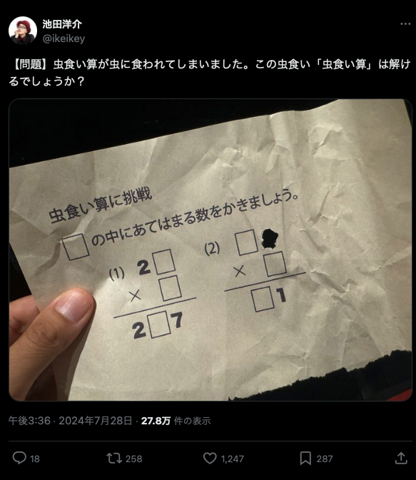
Refer to caption — Figure 3: Screen capture of Yousuke Ikeda’s post [5], proposing a “meta-restoration” puzzle in which a previously restored arithmetic expression is itself damaged again. This screenshot is used with permission from Yousuke Ikeda.

This idea can be generalized naturally to a recursive hierarchy of puzzles (Figure 4). Suppose the erased puzzle was itself a uniquely solvable instance of a prior restoration: this yields a meta-level restoration problem. At level 1, the task is to fill in missing digits in a partially erased arithmetic puzzle, i.e., to solve a standard bookwormed arithmetic. At level 2, some parts of a level-1 puzzle have been bookwormed again, and the goal is to assign digits to these higher-level blanks so that the resulting level-1 puzzle becomes uniquely solvable. This nesting continues: at level $k$ , the solver must assign digits to type- $k$ blanks so that the resulting type- $(k{-}1)$ puzzle admits a unique solution, and so on, all the way down to the base level. Only blanks of the highest type are solved at each level; lower-type blanks remain as part of the sub-instance being reconstructed.

Figure 4: A visual metaphor for meta-level puzzles: each level corresponds to a printout of a uniquely solvable puzzle from the previous level, which is then partially erased. This screenshot has been edited and used with permission from Yosuke Ikeda.

Our main results classify the computational complexity of meta-level puzzles across various settings.

1.

We define a notion of “locally parsimonious reductions” between search problems, and prove that these yield reductions between the meta-level versions of these problems.
2.

In the Boolean satisfiability setting, we show that the level- $k$ SAT problem is complete for the class $\Sigma^{P}_{k}$ . The level- $k$ SAT problem is to decide the truth of quantified Boolean formulae of the form

$\exists x_{1}:\exists!x_{2}:\exists!x_{3}:\dots:\exists!x_{k}:\phi(x_{1},\dots% ,x_{k})$

where each $x_{i}$ denotes a vector of Boolean variables, and $\exists!$ denotes the “exists and is unique” quantifier.
3.

In the arithmetical restoration setting, we show the following partial classification according to which arithmetic operation is involved:

Theorem 1 (Meta-level restorations with multiplication/division).

Let $k\geq 2$ . The level- $k$ meta-restoration problem with multiplication or division is $\Sigma^{P}_{k}$ -complete.

Theorem 2 (Meta-level restorations with addition/subtraction).

The level-2 meta-restoration problem with addition or subtraction is solvable in polynomial time.

As part of showing the latter result, we give a polynomial-time algorithm to determine whether an arithmetical restoration puzzle has a unique solution.

4.

For cryptarithms, we show computational hardness with any of the four arithmetic operations:

Theorem 3 (Meta-level cryptarithms).

Let $k\geq 2$ . The level- $k$ meta-cryptarithm problem with addition, subtraction, multiplication, or division is $\Sigma^{P}_{k}$ -complete.

Along the way to showing these results, we give parsimonious reductions from multiplication to division in arithmetical restorations, and from addition to subtraction, multiplication, or division in cryptarithms. This extends Matsui’s [6] and de Bondt’s [1] results to show ASP-completeness of the corresponding puzzle types.

2 Meta-Level Problems

2.1 Definitions

We define a framework for meta-level problems as follows.

Let $\mathcal{D}$ be a domain, and let $X$ be a set of variables. An assignment $a\in\mathcal{D}^{X}$ is a function assigning each variable in $X$ a value in $\mathcal{D}$ . We can think of a subset $A\subset\mathcal{D}^{X}$ as a solution set to a search problem over the variables $X$ , with each variable taking values in $\mathcal{D}$ .

The level-1 problem corresponding to $A$ is just the ordinary decision problem “Is $A$ nonempty?”. The level- $k$ problem for $k\geq 2$ is specified by assigning each variable in $X$ an integer between 1 and $k$ called its type. The question is whether it is possible to assign values to the type- $k$ variables such that the resulting level- $(k-1)$ problem has a unique solution.

To analyze the computational complexity of such problems, we will consider problems specified by binary strings.

Definition 4.

A search problem $P$ over a domain $\mathcal{D}$ is a function that assigns to each string $s\in\{0,1\}^{*}$ a solution set $P(s)\subset\mathcal{D}^{X}$ , where the set of variables is $X=[|s|]$ .¹¹1We make the set $X$ of variables explicit in this definition, but the point is that the number of variables is polynomially related to the size of the instance.

Note that the domain $\mathcal{D}$ will commonly be infinite: for example, in arithmetic restoration the domain is $\mathbb{N}$ since each variable represents a digit in the base specified by the problem instance.

Definition 5.

Let $P$ be a search problem and $k\geq 1$ be an integer. The level- $k$ $P$ problem is the language of strings $(s,t)$ such that the formula

\exists v_{k}:\exists!v_{k-1}:\exists!v_{k-2}:\dots:\exists!v_{1}:[v\in P(s)]

is satisfied, where $t$ encodes a function from $X=[|s|]$ to $\{1,\dots,k\}$ , and $v_{i}$ is the list of variables $x$ of type $t(x)=i$ .

2.2 Reductions between Meta-Level Versions of Constraint Satisfaction Problems

Now we define a type of reductions between search problems which will turn out to lift to reductions between the level- $k$ versions of those problems.

Definition 6.

Let $A\subset\mathcal{D}^{X}$ and $B\subset\mathcal{E}^{Y}$ be solution sets over the domains $\mathcal{D}$ and $\mathcal{E}$ respectively. We say that $B$ locally reproduces $A$ if there is a bijection $f:A\to B$ with the following properties:

First, for each variable $x\in X$ there must exist a corresponding set of variables $S_{x}\subset Y$ , and an injection $f_{x}:V_{x}\to\mathcal{E}^{S_{x}}$ where $V_{x}=\{a[x]:a\in A\}$ is the set of all possible values taken by the variable $x$ as part of a solution $a\in A$ . The sets $S_{x}$ are required to be disjoint from each other.

Second, the bijection $f$ must satisfy the equation $f(a)[y]=f_{x}(a[x])[y]$ for every assignment $a\in A$ and each pair of variables $x\in X,y\in S_{x}$ .

The definition states that the values of the variables $S_{x}$ in $f(a)$ depend only on the value of $x$ in $a$ . Another phrasing is that the function $a\mapsto f(a)|_{\bigcup_{x}{S_{x}}}$ is the product of the functions $f_{x}$ .

More generally, let $X^{\prime}\subset X$ , and write $Y^{\prime}=\bigcup_{x\in X^{\prime}}S_{x}$ . Define the sets $V_{X^{\prime}}\subset\mathcal{D}^{X^{\prime}},W_{Y^{\prime}}\subset\mathcal{E}% ^{Y^{\prime}}$ by $V_{X^{\prime}}=\{a|_{X^{\prime}}:a\in A\}$ and $W_{Y^{\prime}}=\{b|_{Y^{\prime}}:b\in B\}$ ; these are the sets of feasible partial assignments to $X^{\prime}$ (respectively, $Y^{\prime}$ ) which can be extended to an assignment in $A$ (respectively, $B$ ). We write $\tilde{f}_{X^{\prime}}:V_{X^{\prime}}\to\mathcal{E}^{Y^{\prime}}$ for the product function $\tilde{f}_{X^{\prime}}=\prod_{x\in X^{\prime}}f_{x}$ .

Lemma 7.

The function $\tilde{f}_{X^{\prime}}$ is in fact a bijection $\tilde{f}_{X^{\prime}}:V_{X^{\prime}}\to W_{Y^{\prime}}$ .

Proof.

We prove that $\tilde{f}_{X^{\prime}}$ always outputs an element of $W_{Y^{\prime}}$ , that it is injective, and that it is surjective on $W_{Y^{\prime}}$ .

First, consider an arbitrary element of $V_{X^{\prime}}$ ; it can be written as $a|_{X^{\prime}}$ for some $a\in A$ . Then $\tilde{f}_{X^{\prime}}(a|_{X^{\prime}})$ is equal to $f(a)|_{Y^{\prime}}$ , and the latter is in $W_{Y^{\prime}}$ because $f(a)\in B$ . So $\tilde{f}_{X^{\prime}}$ always outputs an element of $W_{Y^{\prime}}$ .

Second, $\tilde{f}_{X^{\prime}}$ is injective because it is the product of the injective functions $f_{x}$ .

Third, consider an arbitrary element of $W_{Y^{\prime}}$ ; it can be written as $b|_{Y^{\prime}}$ for some $b\in B$ . Then $\tilde{f}_{X^{\prime}}(f^{-1}(b)|_{X^{\prime}})=b|_{Y^{\prime}}$ , so $\tilde{f}_{X^{\prime}}$ is surjective onto $W_{Y^{\prime}}$ . $\hfill\blacktriangleleft$

The purpose of Definition 6 is to prove the following:

Lemma 8.

Let $A\subset\mathcal{D}^{X}$ and $B\subset\mathcal{E}^{Y}$ be solution sets, and $t:X\to\{1,\dots,k\}$ be a function assigning types to the variables in $X$ . Suppose $B$ locally reproduces $A$ , so there exist $f,f_{x},S_{x}$ as in Definition 6.

Assign types to the variables in $Y$ according to the function

t^{\prime}(y)=\begin{cases}t(x)&\text{if $y\in S_{x}$ for some $x\in X$}\\ 1&\text{otherwise.}\\ \end{cases}

Now fix $j\in\{1,\dots,k\}$ , and let $X_{>j}$ and $Y_{>j}$ be the sets of variables in $X$ and $Y$ (respectively) of type strictly greater than $j$ .

Suppose $a\in V_{X_{>j}}$ is a feasible partial assignment to $X_{>j}$ . Then the equivalences

	$\displaystyle\mathrel{\phantom{\iff}}\Bigl(\exists!v_{j}:\exists!v_{j-1}:\dots% :\exists!v_{1}:[a\\|v_{j}\\|\dots\\|v_{1}\in A]\Bigr)$
	$\displaystyle\iff\Bigl(\exists!w_{j}:\exists!w_{j-1}:\dots:\exists!w_{1}:[% \tilde{f}_{X_{>j}}(a)\\|w_{j}\\|\dots\\|w_{1}\in B]\Bigr)$

and

	$\displaystyle\mathrel{\phantom{\iff}}\Bigl(\exists v_{j}:\exists!v_{j-1}:\dots% :\exists!v_{1}:[a\\|v_{j}\\|\dots\\|v_{1}\in A]\Bigr)$
	$\displaystyle\iff\Bigl(\exists w_{j}:\exists!w_{j-1}:\dots:\exists!w_{1}:[% \tilde{f}_{X_{>j}}(a)\\|w_{j}\\|\dots\\|w_{1}\in B]\Bigr)$

both hold, where $v_{i}$ is the list of variables in $X$ of type $i$ , $w_{i}$ is the list of variables in $Y$ of type $i$ , and $\|$ denotes combination of assignments to disjoint sets of variables.

Proof.

The proof is by induction on $j$ . We write $X_{=j}$ and $Y_{=j}$ for the sets of type- $j$ variables in $X$ and $Y$ respectively. Note that by definition of $t^{\prime}$ we have $Y_{=j}=\bigcup_{x\in X_{=j}}S_{x}$ except when $j=1$ .

Let $j=1$ , and fix a feasible partial assignment $a$ to $X_{>1}$ . We exhibit a bijection between the sets $\{c_{1}:a\|c_{1}\in A\}$ and $\{d_{1}:\tilde{f}_{X_{>1}}(a)\|d_{1}\in B\}$ . The bijection is given by $c_{1}\mapsto f(a\|c_{1})|_{Y_{=1}}$ , whose inverse is $d_{1}\mapsto f^{-1}(\tilde{f}_{X_{>1}}(a)\|d_{1})|_{X_{=1}}$ . So these sets have the same size, which means the formulae in the lemma statement are equivalent.

Now let $j>1$ , and fix a feasible partial assignment $a$ to $X_{>j}$ . Suppose $c_{j}$ is a partial assignment to $X_{=j}$ such that $a\|c_{j}$ is feasible. Then by the inductive hypothesis, the formula

\exists!v_{j-1}:\dots:\exists!v_{1}:[a\|c_{j}\|v_{j-1}\|\dots\|v_{1}\in A]

(1)

is equivalent to

\exists!w_{j-1}:\dots:\exists!w_{1}:[\tilde{f}_{X_{>j-1}}(a\|c_{j})\|w_{j-1}\|% \dots\|w_{1}\in B].

Since $\tilde{f}_{X_{>j-1}}(a\|c_{j})=\tilde{f}_{X_{>j}}(a)\|\tilde{f}_{X_{=j}}(c_{j})$ , it follows using Lemma 7 that $\tilde{f}_{X_{=j}}$ is a bijection between partial assignments $c_{j}$ satisfying the formula (1) and partial assignments $d_{j}$ to $Y_{=j}$ satisfying

\exists!w_{j-1}:\dots:\exists!w_{1}:[\tilde{f}_{X_{>j}}(a)\|d_{j}\|w_{j-1}\|% \dots\|w_{1}\in B].

In particular, the number of such $c_{j}$ is equal to the number of such $d_{j}$ , which proves the lemma statement. $\hfill\blacktriangleleft$

Using this lemma, we can define our desired reductions between search problems.

Definition 9.

Let $P$ and $Q$ be search problems. A locally parsimonious reduction from $P$ to $Q$ is a function $g:\{0,1\}^{*}\to\{0,1\}^{*}$ such that $Q(g(s))$ locally reproduces $P(s)$ for each $s\in\{0,1\}^{*}$ , and the sets $S_{x}$ can be computed in polynomial time.

Many existing parsimonious reductions are in fact locally parsimonious. For instance, this is true for the reduction from SAT to 3SAT given in [9], since every SAT variable is given a single corresponding 3SAT variable. The same holds for the reduction from SAT to 1-in-3SAT.

Theorem 10.

Let $P$ and $Q$ be search problems over the domains $\mathcal{D}$ and $\mathcal{E}$ respectively, and $g$ be a locally parsimonious reduction from $P$ to $Q$ . Then there is a polynomial-time reduction from the level- $k$ $P$ problem to the level- $k$ $Q$ problem.

Proof.

Let $(s,t)$ be an instance of the level- $k$ $P$ problem. We define the output of the reduction to be $(g(s),t^{\prime})$ where $t^{\prime}$ is defined as in Lemma 8. It follows immediately from Lemma 8, that $(s,t)$ is a YES instance if and only if $(g(s),t^{\prime})$ is. $\hfill\blacktriangleleft$

Combined with the results of the next section, Theorem 10 can be used to show $\Sigma^{P}_{k}$ -hardness for the level- $k$ version of a problem by finding a locally parsimonious reduction from SAT (or 3SAT, or 1-in-3SAT) to that problem. Similarly, containment in $\Sigma^{P}_{k}$ can be shown by finding a locally parsimonious reduction in the other direction.

3 $\Sigma^{P}_{k}$ -Completeness of Level- $𝒌$ SAT

In this section, we prove that level- $k$ SAT is $\Sigma^{P}_{k}$ -complete.

Theorem 11 (Level- $𝒌$ SAT is $\Sigma^{P}_{k}$ -complete).

For every $k\geq 1$ , the satisfiability problem for formulae of the form $\exists x_{1}:\exists!x_{2}:\exists!x_{3}:\cdots:\exists!x_{k}:\phi(x_{1},% \dots,x_{k})$ , where each $x_{i}$ denotes a vector of Boolean variables, is $\Sigma^{P}_{k}$ -complete.

Proof of Theorem 11.

We claim that any formula of the form $\exists!x_{1}:\exists!x_{2}:\cdots:\exists!x_{k}:\phi(x_{1},\dots,x_{k},z)$ , where $x_{i},z$ are vectors of Boolean variables and $z$ is free, can be transformed in polynomial time into two equivalent Boolean formulae with $k+1$ blocks of alternating quantifiers: one starting with $\exists$ and the other starting with $\forall$ . We refer to these two desired forms as the “ $\Sigma^{P}_{k+1}$ form” and the “ $\Pi^{P}_{k+1}$ form” respectively.

The proof is by induction on $k$ . The key observation is that each uniqueness quantifier $\exists!x$ can be rewritten using standard quantifiers in two different ways:

	( $\exists\,\forall$ rewriting)	$\displaystyle\exists!x:\psi(x)\iff\exists x:\forall x^{\prime}:[\psi(x)\land(% \psi(x^{\prime})\rightarrow x^{\prime}=x)],$
	( $\forall\,\exists$ rewriting)	$\displaystyle\exists!x:\psi(x)\iff\forall x^{\prime}_{1}:\forall x^{\prime}_{2% }:\exists x:[\psi(x)\land((\psi(x^{\prime}_{1})\land\psi(x^{\prime}_{2}))% \rightarrow x^{\prime}_{1}=x^{\prime}_{2})].$

Let $\psi(x_{1})=\exists!x_{2}:\cdots:\exists!x_{k}:\phi(x_{1},\dots,x_{k},z)$ . By the inductive hypothesis, we can rewrite $\psi(x_{1})$ in both $\Sigma^{P}_{k}$ form and $\Pi^{P}_{k}$ form. To write $\exists!x_{1}:\psi(x_{1})$ in $\Sigma^{P}_{k+1}$ form, we apply the $\exists\forall$ rewriting above. We then replace the positive occurrence of $\psi(x_{1})$ with its $\Pi^{P}_{k}$ form and the negative occurrence of $\psi(x_{1})$ with its $\Sigma^{P}_{k}$ form. After applying De Morgan’s laws and the equivalences

	$\displaystyle(\forall x:\phi_{0}(x))\land(\forall x:\phi_{1}(x))$	$\displaystyle\iff\forall x:\forall b\in\{0,1\}:(b=0\to\phi_{0}(x))\land(b=1\to% \phi_{1}(x))$
	$\displaystyle(\forall x:\phi_{0}(x))\lor(\forall x:\phi_{1}(x))$	$\displaystyle\iff\forall x_{0}:\forall x_{1}:\phi_{0}(x_{0})\lor\phi_{1}(x_{1})$

to move all quantifiers to the beginning, the result is a formula in $\Sigma^{P}_{k+1}$ form. Finding the $\Pi^{P}_{k+1}$ form is analogous, but we use the $\forall\exists$ rewriting and make the opposite choices for $\psi(x_{1})$ . These rewriting steps take polynomial time,²²2The time taken and the size of the output formula are both exponential in the constant $k$ , but polynomial in the size of the input formula. so the claim is proved. It follows from this that satisfiability of formulae of the form $\exists x_{1}:\exists!x_{2}:\cdots:\exists!x_{k}:\phi(x_{1},\dots,x_{k})$ is contained in $\Sigma^{P}_{k}$ , simply by rewriting $\exists!x_{2}:\cdots:\exists!x_{k}:\phi(x_{1},\dots,x_{k})$ in $\Sigma^{P}_{k}$ form.

It remains to show $\Sigma^{P}_{k}$ -hardness. Consider any formula of the form $\neg\exists x_{1}:\neg\exists x_{2}:\cdots:\neg\exists x_{k}:\phi(x_{1},\dots,% x_{k},z)$ where $x_{i},z$ are vectors of Boolean variables and $z$ is free. An induction on $k$ shows that this formula is equivalent to

	$\displaystyle\exists!(x_{1},a_{1}):\exists!(x_{2},a_{2}):\cdots:\exists!(x_{k}% ,a_{k}):$
	$\displaystyle\left(\bigwedge_{i=2}^{k}(a_{i-1}\to a_{i})\right)\land\left(% \bigwedge_{i=1}^{k}(a_{i}\to x_{i}=\langle 0,\ldots,0\rangle)\right)\land\left% (\phi(x_{1},\dots,x_{k},z)\lor\bigvee_{i=1}^{k}a_{i}\right),$

where each $a_{i}$ is a single Boolean variable. Proof by induction:
$\displaystyle\mathrel{\phantom{\iff}}\left[\begin{gathered}\exists!(x_{1},a_{1% }):\exists!(x_{2},a_{2}):\cdots:\exists!(x_{k},a_{k}):\\ \left(\bigwedge_{i=2}^{k}(a_{i-1}\to a_{i})\right)\land\left(\bigwedge_{i=1}^{% k}(a_{i}\to x_{i}=\langle 0,\ldots,0\rangle)\right)\land\left(\phi(x_{1},\dots% ,x_{k},z)\lor\bigvee_{i=1}^{k}a_{i}\right)\end{gathered}\right]$ $\displaystyle\iff\begin{gathered}\exists!(x_{1},a_{1}):\\ \begin{cases}\left[\begin{gathered}\exists!(x_{2},a_{2}):\cdots:\exists!(x_{k}% ,a_{k}):\\ \left(\bigwedge_{i=3}^{k}(a_{i-1}\to a_{i})\right)\land\left(\bigwedge_{i=2}^{% k}(a_{i}\to x_{i}=\langle 0,\ldots,0\rangle)\right)\land\left(\phi(x_{1},\dots% ,x_{k},z)\lor\bigvee_{i=2}^{k}a_{i}\right)\end{gathered}\right]\\ \hfill\text{if }a_{1}=0\\ \left[\begin{gathered}\exists!(x_{2},a_{2}):\cdots:\exists!(x_{k},a_{k}):\\ \left(\bigwedge_{i=2}^{k}a_{i}=1\right)\land\left(\bigwedge_{i=1}^{k}x_{i}=% \langle 0,\ldots,0\rangle\right)\end{gathered}\right]\hfill\text{if }a_{1}=1% \end{cases}\end{gathered}$ $\displaystyle\iff\exists!(x_{1},a_{1}):\begin{cases}\neg\exists x_{2}:\neg% \exists x_{3}:\cdots:\neg\exists x_{k}:\phi(x_{1},\dots,x_{k},z)&\text{if }a_{% 1}=0\\ x_{1}=\langle 0,\ldots,0\rangle&\text{if }a_{1}=1\end{cases}$ $\displaystyle\iff\neg\exists x_{1}:\neg\exists x_{2}:\cdots:\neg\exists x_{k}:% \phi(x_{1},\dots,x_{k},z)$

Since satisfiability of formulae of the form $\exists x_{1}:\neg\exists x_{2}:\neg\exists x_{3}:\cdots:\neg\exists x_{k}:% \phi(x_{1},\dots,x_{k})$ is $\Sigma^{P}_{k}$ -complete, it follows from the above that satisfiability of formulae of the form $\exists x_{1}:\exists!x_{2}:\exists!x_{3}:\cdots:\exists!x_{k}:\phi(x_{1},% \dots,x_{k})$ is $\Sigma^{P}_{k}$ -complete also, by rewriting the rest of the formula after the first quantifier. $\hfill\blacktriangleleft$

4 Arithmetic Puzzles: Definitions

4.1 Arithmetical Restorations

In order to formalize arithmetical restorations, we focus here on addition, which is the primary case where tractability arises. Other operations (subtraction, multiplication, and division) are treated analogously but lead to different complexity classifications, as discussed later.

An instance $X_{+}$ consists of two $m$ -digit addends and their sum in base $n$ , possibly of length $m$ or $m+1$ . To streamline notation, we include two boundary columns: $C_{0}=(0,0,0)$ and $C_{m+1}=(0,0,\alpha)$ with $\alpha\in\{0,1\}$ , resulting in $m+2$ columns in total: $C_{m+1},C_{m},\dots,C_{0}$ (see Figure 6). Each internal column $C_{i}$ ( $1\leq i\leq m$ ) consists of a triple $(c_{i}^{1},c_{i}^{2},c_{i}^{3})$ , where $c_{i}^{1}$ and $c_{i}^{2}$ are the digits to be added, and $c_{i}^{3}$ is the corresponding digit of the sum.

Figure 5: Basic layout of an arithmetical restoration for addition.

Figure 6: Formal structure of the addition puzzle.

Let $x_{1},\dots,x_{k}$ be the variables in $X_{+}$ . For an assignment $s\in\{0,\dots,n{-}1\}^{k}$ , let $X_{+}(s)$ denote the resulting table after substitution. An assignment $s$ is a solution if $X_{+}(s)$ satisfies the addition rule with proper carry propagation. Evaluation proceeds from the least significant digit (rightmost column) to the most significant digit, propagating carries according to:

\mathrm{Carry}(C_{i}(s)):=\begin{cases}0&\text{if }c^{1}_{i}+c^{2}_{i}+\mathrm% {Carry}(C_{i-1}(s))<n\\ 1&\text{otherwise}.\end{cases}

4.2 Cryptarithms

Cryptarithms are puzzles in which digits are replaced by letters. The goal is to assign distinct digits to letters so that the resulting arithmetic expression is valid. We focus on multiplication; other operations follow analogous definitions. An instance $Y_{\times}$ consists of:

1.

a multiplicand $S_{1}$ of length $p$ ,
2.

a multiplier $S_{2}$ of length $q$ ,
3.

$q$ partial products $S_{i}$ of length $\ell_{i}$ with $3\leq i\leq q+2$ , where $1\leq\ell_{i}\leq p+1$ , and
4.

a final product $S_{q+3}$ of length $1\leq\ell_{q+3}\leq pq+1$ .

Let $S$ be the set of letters used in $Y_{\times}$ . A digit assignment $s:S\to\{0,\dots,n{-}1\}$ induces a concrete puzzle $Y_{\times}(s)$ via substitution. An assignment $s$ is a solution if:

1.

all arithmetic operations in $Y_{\times}(s)$ are correct in base $n$ , and
2.

all digits assigned are pairwise distinct.

Figure 7: Structure of a multiplication cryptarithm.

5 Arithmetic Puzzles: Hardness

5.1 Parsimonious Reductions Across Arithmetic Operations

We now show that arithmetical restoration and cryptarithm puzzles involving subtraction, multiplication, and division are all ASP-complete.

Lemma 12 (ASP-completeness across operations).

Arithmetical restorations with multiplication or division are ASP-complete. Cryptarithms with subtraction, multiplication, or division are also ASP-complete. Thus the corresponding counting problems are #P-complete.

To prove Lemma 12, we systematically construct parsimonious reductions between puzzle types and operations. These reductions preserve the number of solutions, allowing us to transfer the known hardness of addition and multiplication to subtraction and division. We divide the proof into four parts, each showing a parsimonious reduction between two operations.

Reduction from Multiplication to Division in Restorations.

Matsui [6] showed that the arithmetical restoration problem with multiplication is ASP-complete via a reduction from Monotone 1-in-3SAT. The instance $X_{\times}$ consists of digit sequences $S_{A}$ , $S_{B}$ , $S_{C}$ , and $S_{1},\ldots,S_{q}$ arranged to represent a multiplication table.

Figure 8 illustrates the structure of $X_{\times}$ .

Figure 8: Multiplication instance

X_{\times}

reduced from Monotone 1-in-3SAT [6].

Figure 9: Division instance

X_{\div}

constructed from the multiplication instance

X_{\times}

.

To reduce to division, we construct a new instance $X_{\div}$ that reuses these sequences in a division layout. We add auxiliary rows $S^{\prime}_{1},\ldots,S^{\prime}_{q}$ to account for intermediate subtractions. Each subtraction step in the division corresponds to a row in the multiplication layout, preserving the structure of the solution.

Fixing the divisor and quotient uniquely determines all subtraction steps, so the number of solutions is preserved. Thus, the reduction is parsimonious.

Reduction from Addition to Subtraction in Cryptarithms.

Let $Y_{+}(\phi)$ be the cryptarithm with addition derived from a Positive 1-in-3SAT instance. It consists of three rows: $G_{1}+G_{2}=G_{3}$ .

We construct $Y_{-}(\phi)$ by rearranging the rows as $G_{3}-G_{2}=G_{1}$ and changing the operator to subtraction. This transformation preserves the solution space, due to the symmetry between carry and borrow behavior in digit gadgets.

(a)

(b)

(c)

(d)

Figure 10: Carry-borrow symmetry in digit gadgets under row-swapping.

Reduction from Addition to Multiplication in Cryptarithms.

We embed the structure of $Y_{+}(\phi)$ into a multiplication layout to form $Y_{\times}(\phi)$ . Fixed digits $c_{0}=0$ and $c_{1}=1$ are introduced to maintain constant semantics. The region corresponding to $G_{1}+G_{2}=G_{3}$ is preserved within the multiplicative table layout.

Figure 11: Reduction from cryptarithm addition

Y_{+}(\phi)

to multiplication

Y_{\times}(\phi)

.

Figure 12: Reduction from cryptarithm subtraction

Y_{-}(\phi)

to division

Y_{\div}(\phi)

.

This transformation embeds the original constraint structure without ambiguity, ensuring a one-to-one correspondence of solutions.

Reduction from Subtraction to Division in Cryptarithms.

Finally we reduce cryptarithm subtraction to division by embedding the instance $Y_{-}(\phi)$ into a division layout. We reuse the row configuration $G_{3}-G_{2}=G_{1}$ to form a long division table $Y_{\div}(\phi)$ , fixing $c_{0}=0$ and $c_{1}=1$ as constants.

The core structure is preserved inside a designated region, and all auxiliary digits are placed disjointly to avoid interference. The transformation is again parsimonious.

This completes the proof of Lemma 12.

5.2 Meta-Level Complexity

We now complete the classification of meta-level puzzles by proving Theorem 1 and Theorem 3, which concern the complexity of multiplicative meta-restorations and meta-cryptarithms, respectively.

We accomplish this by applying the results of Section 2.2 to the preceding parsimonious reductions, allowing us to obtain reductions between the meta-level versions of the problems. Indeed, from the structure of the reductions it is clear that every variable of the input instance corresponds to a single variable of the output instance, so the reductions are in fact locally parsimonious. The same is true for the reductions of [4, 6, 1] used to show ASP-completeness of arithmetical restorations with multiplication and cryptarithms with addition. By Theorems 10 and 11, these reductions show that the preceding problems are $\Sigma^{P}_{k}$ -hard. We can also represent arithmetic restoration and cryptarithms with SAT formulae in a locally parsimonious way, showing containment in $\Sigma^{P}_{k}$ .

Therefore, the meta-restoration and meta-cryptarithm problems are $\Sigma^{P}_{k}$ -complete for all $k\geq 2$ .

6 Arithmetic Puzzles: Algorithms

6.1 Polynomial-Time Algorithms for Arithmetical Restorations with Addition and Subtraction

We prove the following result, which provides a polynomial-time decision algorithm for restorations with addition and subtraction:

Lemma 13 (Additive restorations).

Determining whether a given arithmetical restoration puzzle with addition and subtraction admits a unique solution is in $P$ .

The basic idea is a dynamic programming approach that focuses on the carry-over values between columns. We first define the corresponding subproblem.

Definition 14 (Extended column feasibility).

Given a column $C_{i}$ and two carry values $(\beta,\alpha)$ , we say that $C_{i}$ is feasible with carries $(\beta,\alpha)$ if there exists an assignment to the variables in $C_{i}$ that is consistent with incoming carry $\beta$ and outgoing carry $\alpha$ .

Lemma 15.

An arithmetical restoration $X_{+}$ has a solution if and only if there exists a sequence $l\in\{0,1\}^{m+1}$ such that, for each $i\in\{1,2,\ldots,m\}$ , the column $C_{i}$ is feasible with carries $(l_{i-1},l_{i})$ .

Proof.

( $\Rightarrow$ ): Suppose $X_{+}$ has a solution $s$ . Let $l=(l_{0},\ldots,l_{m})$ be the carry sequence induced by $s$ , where $l_{i-1}$ is the carry entering column $C_{i}$ and $l_{i}$ the carry leaving it. For each $i$ , the restriction $w_{i}$ of $s$ to $C_{i}$ makes the column feasible with $(l_{i-1},l_{i})$ . Hence the condition holds.
( $\Leftarrow$ ): Conversely, suppose there exists $l$ such that each column $C_{i}$ admits an assignment $w_{i}$ consistent with $(l_{i-1},l_{i})$ . Since the $w_{i}$ concern disjoint sets of variables, their union $s:=\bigcup_{i=1}^{m}w_{i}$ forms a global assignment. By construction, every column constraint is satisfied with the designated carries $l$ , so $s$ is a solution of $X_{+}$ .

$\hfill\blacktriangleleft$

We now develop a column-wise feasibility check for given carry-in and carry-out values, which forms the basis of our algorithm.

Lemma 16.

For a column $C_{i}$ and carry values $(\beta,\alpha)\in\{0,1\}^{2}$ , we can determine in $O(n)$ time whether $C_{i}$ is feasible with carries $(\beta,\alpha)$ .

Proof.

Fix a column $i$ . For each entry $c_{i}^{j}$ in row $j\in\{1,2,3\}$ , define

(x^{j},y^{j}):=\begin{cases}(c_{i}^{j},0)&\text{if }c_{i}^{j}\text{ is type 0}% ,\\ (0,c_{i}^{j})&\text{if }c_{i}^{j}\text{ is type 1}.\end{cases}

From the carry definition, we require: $y^{1}+y^{2}-y^{3}=x^{3}-x^{1}-x^{2}+\alpha n-\beta$ . The left-hand side is a linear expression in at most three variables ranging over $\{0,1,\dots,n-1\}$ , and the right-hand side is constant. The number of variable entries is at most three, and we can compute the range of the left-hand side in constant time by bounding it between $-\theta^{3}(n-1)\quad\text{and}\quad(\theta^{1}+\theta^{2})(n-1)$ , where $\theta^{j}=1$ if $c_{i}^{j}$ is a variable and $0$ otherwise. A feasible assignment exists if and only if the right-hand side lies within this range. $\hfill\blacktriangleleft$

Using this feasibility check, we now describe a polynomial-time algorithm that verifies the existence of a consistent carry sequence across all columns. We construct a directed graph representing feasible carry transitions:

1.

For each $i\in\{0,1,\ldots,m+1\}$ and each $b\in\{0,1\}$ , define a vertex $v_{i,b}$ .
2.

Add an edge from $v_{i-1,\beta}$ to $v_{i,\alpha}$ if column $C_{i}$ admits a feasible assignment with carry-in $\beta$ and carry-out $\alpha$ , as determined by Lemma 16.

Figure 13: Graph structure representing feasible carry transitions.

The total number of vertices is $2(m+2)$ and the number of edges is at most $4(m+1)$ , since each transition layer has at most 4 feasible carry transitions. Each feasibility check runs in $O(n)$ time, and the overall graph construction takes $O(nm)$ time. Finally, we perform a reachability test from $v_{0,0}$ and $v_{0,1}$ to $v_{m+1,0}$ or $v_{m+1,1}$ . This can be done in $O(nm)$ time. Thus, the entire algorithm runs in $O(nm)$ time, proving Lemma 13.

6.2 Polynomial-Time Algorithm for Level-2 Additive Restorations

We now establish Theorem 2 by presenting a polynomial-time algorithm for solving level-2 meta-restorations involving addition or subtraction.

The core idea is to extend the level-1 restoration algorithm, which checks the consistency of a partially erased addition table, to also verify uniqueness – a requirement at level 2. To this end, we construct a directed graph that captures all valid and unique carry-over transitions across columns.

Specifically, let each vertex $v_{i,b}$ represent the carry value $b\in\{0,1\}$ at column index $i$ (from right to left). We add an edge $v_{i-1,b}\to v_{i,b^{\prime}}$ if there exists an assignment to the type-2 entries of column $C_{i}$ such that there exists a unique way to fill in the type-1 entries of column $C_{i}$ such that:

1.

the incoming carry is $b$ and the outgoing carry is $b^{\prime}$ ,
2.

the assignment respects the roles of the cells (type-0: fixed, type-1: blank at level 1, type-2: blank at level 2), and
3.

the assignment is consistent with addition modulo $n$ .

We can then decide solvability by checking whether this graph contains a valid path from the leftmost vertex (typically $v_{0,0}$ ) to the rightmost vertex (typically $v_{\ell,0}$ , where $\ell$ is the number of columns).

The following lemma underpins the tractability of the edge construction step:

Lemma 17.

Fix a column $C_{i}$ with given carry-in $\beta$ and carry-out $\alpha$ . We can determine in $O(n)$ time whether there exists an assignment to the type-2 variables in $C_{i}$ (if any) such that the values of all type-1 variables in $C_{i}$ are uniquely determined and the column is consistent.

Proof.

Fix a column $C_{i}$ with carry-in $\beta$ and carry-out $\alpha$ .

Let $c_{i}^{1},c_{i}^{2},c_{i}^{3}$ denote the three entries of column $C_{i}$ . Each $c_{i}^{j}$ is interpreted as follows: if it is of type 0, then $c_{i}^{j}$ is the fixed digit given in the puzzle; if it is of type 1 or type 2, then $c_{i}^{j}$ denotes the corresponding variable to be assigned. For each row $j\in\{1,2,3\}$ , define:

(x^{j},y^{j},z^{j}):=\begin{cases}(c_{i}^{j},0,0)&\text{if }c_{i}^{j}\text{ is% type 0},\\ (0,c_{i}^{j},0)&\text{if }c_{i}^{j}\text{ is type 1},\\ (0,0,c_{i}^{j})&\text{if }c_{i}^{j}\text{ is type 2}.\end{cases}

From the semantics of additive restoration with carries, we require:

z^{1}+z^{2}-z^{3}=x^{3}+y^{3}-x^{1}-x^{2}-y^{1}-y^{2}+\alpha n-\beta.

Let $C:=x^{1}+x^{2}-x^{3}-\alpha n+\beta$ , which is fully determined by type-0 entries and carry values.

We distinguish cases according to the presence/absence of type-1 and type-2 entries in the column:

(1)

All of $c_{i}^{1},c_{i}^{2},c_{i}^{3}$ are not type-2. In this case, it suffices to check whether the type-1 variables admit a unique assignment, which can be done by a straightforward extension of Lemma 16.
(2)

All of $c_{i}^{1},c_{i}^{2},c_{i}^{3}$ are not type-1. In this case, there are no type-1 variables, so uniqueness holds vacuously. We only need to check whether there exists an assignment to the type-2 variables that makes the column consistent. This can be done by treating all type-2 variables as type-1 variables and applying Lemma 16.
(3)

Exactly one of $c_{i}^{1},c_{i}^{2},c_{i}^{3}$ is a type-1 variable. In this case, equation (6.2) becomes $C+z^{1}+z^{2}-z^{3}=y^{3}-y^{1}-y^{2}.$ The right-hand side can only take a restricted range of values: if $y^{3}$ is the type-1 variable, then it ranges over $[0,n-1]$ ; if $y^{1}$ or $y^{2}$ is the type-1 variable, then it ranges over $[-(n-1),0]$ . Thus the feasibility reduces to checking whether one can assign values to at most two type-2 variables among $z^{1},z^{2},z^{3}$ so that the left-hand side falls into the corresponding range. This can be decided in polynomial time by the same idea as in Lemma 16.
(4)
Exactly two of $c_{i}^{1},c_{i}^{2},c_{i}^{3}$ are type-1 variables. In this case, equation (6.2) becomes $C+z^{1}+z^{2}-z^{3}=y^{3}-y^{1}-y^{2}.$ There are two subcases:
1. (i)
  
  $y^{3}=0$ and both $y^{1},y^{2}$ are type-1. Then the equation reduces to $C+z^{1}+z^{2}-z^{3}=-(y^{1}+y^{2})$ . The pair $(y^{1},y^{2})$ is uniquely determined only if the right-hand side is $0$ or $-2(n-1)$ , yielding $(y^{1},y^{2})=(0,0)$ or $(n-1,n-1)$ .
2. (ii)
  
  $y^{1}=0$ (without loss of generality) and $y^{2},y^{3}$ are type-1. Then the equation becomes $C+z^{1}+z^{2}-z^{3}=y^{3}-y^{2}$ . The pair $(y^{2},y^{3})$ is uniquely determined only if the right-hand side is $n-1$ or $-(n-1)$ , which forces $(y^{2},y^{3})=(0,n-1)$ or $(y^{2},y^{3})=(n-1,0)$ .
Thus the decision reduces to checking whether the unique type-2 variable among $z^{1},z^{2},z^{3}$ can be assigned so that the left-hand side matches one of these special values. This check can be performed in polynomial time by the same idea as in Lemma 16.

$\hfill\blacktriangleleft$ By applying Lemma 17 to each candidate edge, we can construct the graph in polynomial time. Reachability in this graph determines whether a globally consistent and unique assignment exists, completing the algorithm for level-2 restorations.

7 Open Questions

We conclude with some open questions.

1.

In this paper we explored the complexity of formulae involving nested $\exists!x$ quantifiers. What can be said about other similar types of quantifiers? For instance, we could consider quantifiers such as “there exist exactly two $x$ satisfying $P(x)$ ” and “exactly half of all $x$ satisfy $P(x)$ ”.
2.

Are there natural examples of parsimonious reductions that are not locally parsimonious?
3.

Regarding the hardness of meta-level additive restorations: While we have shown that level-2 additive restorations admit a polynomial-time algorithm, the computational complexity of level- $k$ additive or subtractive restorations for $k>2$ remains open. Do such problems climb higher in the polynomial hierarchy, or can they still be solved efficiently?

References

[1] Michael de Bondt. On the ASP-completeness of cryptarithms. Technical Report 0419, Department of Mathematics, Radboud University, Nijmegen, Netherlands, November 2004. URL: https://hdl.handle.net/2066/60283.
[2] David Eppstein. On the NP-completeness of cryptarithms. ACM SIGACT News, 18(3):38–40, 1987. doi:10.1145/24658.24662.
[3] Kozaburo Fujimura. Puzzles and Problems (in Japanese). Diamond Sha Co., Ltd., 1969.
[4] Harry B. Hunt, Madhav V. Marathe, Venkatesh Radhakrishnan, and Richard E. Stearns. The complexity of planar counting problems. SIAM Journal on Computing, 27(4):1142–1167, 1998. doi:10.1137/S0097539793304601.
[5] Yousuke Ikeda. X post on July 28, 2024. https://x.com/ikeikey/status/1817448938322202776. Accessed: 2024-09-21.
[6] Tomomi Matsui. NP-completeness of arithmetical restorations. Journal of Information Processing, 21(3):402–404, July 2013. doi:10.2197/IPSJJIP.21.402.
[7] Ryuhei Uehara. Computational complexity of puzzles and related topics. Interdisciplinary Information Sciences, 29(2):1–23, 2023. doi:10.4036/iis.2022.R.06.
[8] Ryuhei Uehara. Algorithms for Puzzles (in Japanese). Nippon Hyoron Sha Co., Ltd., 2024.
[9] Takayuki Yato and Takahiro Seta. Complexity and completeness of finding another solution and its application to puzzles. IEICE Transactions on Fundamentals of Electronics, Communications, and Computer Sciences, E86-A(5):1052–1060, 2003. Also IPSJ SIG Notes 2002-AL-87-2, 2002. URL: http://ci.nii.ac.jp/naid/110003221178/en/.

[bib.bib1] [1] Michael de Bondt. On the ASP-completeness of cryptarithms. Technical Report 0419, Department of Mathematics, Radboud University, Nijmegen, Netherlands, November 2004. URL: https://hdl.handle.net/2066/60283.

[bib.bib2] [2] David Eppstein. On the NP-completeness of cryptarithms. ACM SIGACT News, 18(3):38–40, 1987. doi:10.1145/24658.24662.

[bib.bib3] [3] Kozaburo Fujimura. Puzzles and Problems (in Japanese). Diamond Sha Co., Ltd., 1969.

[bib.bib4] [4] Harry B. Hunt, Madhav V. Marathe, Venkatesh Radhakrishnan, and Richard E. Stearns. The complexity of planar counting problems. SIAM Journal on Computing, 27(4):1142–1167, 1998. doi:10.1137/S0097539793304601.

[bib.bib5] [5] Yousuke Ikeda. X post on July 28, 2024. https://x.com/ikeikey/status/1817448938322202776. Accessed: 2024-09-21.

[bib.bib6] [6] Tomomi Matsui. NP-completeness of arithmetical restorations. Journal of Information Processing, 21(3):402–404, July 2013. doi:10.2197/IPSJJIP.21.402.

[bib.bib7] [7] Ryuhei Uehara. Computational complexity of puzzles and related topics. Interdisciplinary Information Sciences, 29(2):1–23, 2023. doi:10.4036/iis.2022.R.06.

[bib.bib8] [8] Ryuhei Uehara. Algorithms for Puzzles (in Japanese). Nippon Hyoron Sha Co., Ltd., 2024.

[bib.bib9] [9] Takayuki Yato and Takahiro Seta. Complexity and completeness of finding another solution and its application to puzzles. IEICE Transactions on Fundamentals of Electronics, Communications, and Computer Sciences, E86-A(5):1052–1060, 2003. Also IPSJ SIG Notes 2002-AL-87-2, 2002. URL: http://ci.nii.ac.jp/naid/110003221178/en/.

A Bookworm Climbs up the Polynomial Hierarchy: Meta-Restoration Complexity in Arithmetic Puzzles

Abstract

Keywords and phrases:

Copyright and License:

2012 ACM Subject Classification:

DOI:

Event:

Editor:

Series and Publisher:

1 Introduction

Theorem 1 (Meta-level restorations with multiplication/division).

Theorem 2 (Meta-level restorations with addition/subtraction).

Theorem 3 (Meta-level cryptarithms).

2 Meta-Level Problems

2.1 Definitions

Definition 4.

Definition 5.

2.2 Reductions between Meta-Level Versions of Constraint Satisfaction Problems

Definition 6.

Lemma 7.

Proof.

Lemma 8.

Proof.

Definition 9.

Theorem 10.

Proof.

3 𝚺𝒌𝑷-Completeness of Level-𝒌 SAT

Theorem 11 (Level-𝒌 SAT is 𝚺𝒌𝑷-complete).

Proof of Theorem 11.

4 Arithmetic Puzzles: Definitions

4.1 Arithmetical Restorations

4.2 Cryptarithms

5 Arithmetic Puzzles: Hardness

5.1 Parsimonious Reductions Across Arithmetic Operations

Lemma 12 (ASP-completeness across operations).

Reduction from Multiplication to Division in Restorations.

Reduction from Addition to Subtraction in Cryptarithms.

Reduction from Addition to Multiplication in Cryptarithms.

Reduction from Subtraction to Division in Cryptarithms.

5.2 Meta-Level Complexity

6 Arithmetic Puzzles: Algorithms

6.1 Polynomial-Time Algorithms for Arithmetical Restorations with Addition and Subtraction

Lemma 13 (Additive restorations).

Definition 14 (Extended column feasibility).

Lemma 15.

Proof.

Lemma 16.

Proof.

6.2 Polynomial-Time Algorithm for Level-2 Additive Restorations

Lemma 17.

Proof.

7 Open Questions

References

3 $\Sigma^{P}_{k}$ -Completeness of Level- $𝒌$ SAT

Theorem 11 (Level- $𝒌$ SAT is $\Sigma^{P}_{k}$ -complete).