Lozenge Tiling by Computing Distances

Abstract
The Calisson puzzle is a recent tiling game in which one must tile a triangular grid inside a hexagon with lozenges, under the constraint that certain prescribed edges must remain tile boundaries and that adjacent lozenges along these edges have different orientations. We present the first polynomial-time algorithm for this problem, with running time for a hexagon of side length . This algorithm, called the advancing surface algorithm, can be executed in a simple and intuitive way, even by hand with a pencil and an eraser. Its apparent simplicity conceals a deeper algorithmic reinterpretation of the classical ideas of John Conway and William Thurston, which we revisit from a theoretical computer science perspective.
We introduce a graph-theoretic and difference constraints overlay that complements Thurston’s theory of lozenge tilings, revealing its intrinsic algorithmic structure and extending its scope to tiling problems with interior constraints and without necessarily boundary conditions. In Thurston’s approach, lozenge tilings are lifted to monotone stepped surfaces in the three-dimensional cubic lattice and projected back to the plane using height functions, reducing the tiling problem to the computation of heights. We show that, at an algorithmic level, selecting a monotone surface corresponds to selecting a directed cut (dicut) in a periodic directed graph, while height functions are solutions of a system of difference constraints. In this formulation, a region is tilable if and only if the associated weighted directed graph contains no cycle of strictly negative total weight. This new graph layer completing Thurston’s theory shows that Bellman–Ford’s shortest path algorithm is the only algorithmic primitive needed to decide feasibility and compute solutions. In particular, our framework allows us to decide whether the infinite triangular grid can be tiled while respecting a finite set of prescribed local constraints, a setting in which no boundary conditions are available.
Keywords and phrases:
Tiling, Lozenge, Directed Graph, Dicut, Difference Constraints, Bellman-FordFunding:
Pascal Lafourcade: ANR PRC grant SEVERITAS (ANR-20-CE39-0005), ANR Project PRIVA-SIQ (ANR-23-CE39-0008) and IDEX-ISITE initiative 16-IDEX-0001 (CAP 20-25).Copyright and License:
![[Uncaptioned image]](x1.png) © Jean-Marie Favreau, Yan Gerard, Pascal Lafourcade, and Léo Robert; licensed under Creative Commons License CC-BY 4.0
© Jean-Marie Favreau, Yan Gerard, Pascal Lafourcade, and Léo Robert; licensed under Creative Commons License CC-BY 4.0
2012 ACM Subject Classification:
Theory of computation Computational geometryEditor:
John IaconoSeries and Publisher:
 Leibniz International Proceedings in Informatics, Schloss Dagstuhl – Leibniz-Zentrum für Informatik
1 Introduction
Lozenge tilings are found in art, architecture, and monuments around the world. They are universal patterns. In science, their geometric and combinatorial properties have intrigued mathematicians for centuries, drawing the attention of renowned researchers like John Conway and William Thurston in recent decades.
In 2022, Olivier Longuet, a mathematics teacher in a French high school, introduced a geometric logic game called the Calisson puzzle (original name, le jeu du calisson222The name Calisson comes from a traditional French sweet shaped like a lozenge and produced in Aix-en-Provence, a town in the south of France.). The puzzle consists in tiling a hexagonal region of the triangular grid with lozenges subject to local constraints. Olivier Longuet writes a blog (in French) at https://mathix.org/calisson/blog/ where he presents the rules of the puzzle and more than five hundred instances of the game [6]. The game can also be played online at https://martialtarizzo.github.io/Calisson-Game/index.en.html [7].
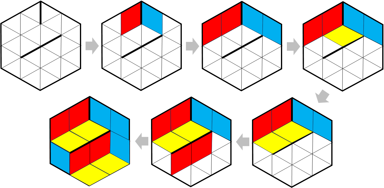
The game is played in a triangular grid bounded by a regular hexagon. The triangular grid contains three classes of edges, depending on their orientation: vertical (the / o’clock direction), the / o’clock direction, and the / o’clock direction. A lozenge is the union of two adjacent unit triangles. Its type is determined by the orientation of the edge shared by the two triangles. There are three types of lozenges, depending on the orientation of their common edge. Lozenges whose common edge is vertical, in the / o’clock direction, or in the / o’clock direction are, for instance, colored respectively in yellow, red, and blue. The rules of the game are simple. They are illustrated in Fig. 1.
Rules of the Calisson puzzle
Input: A triangular grid bounded by a regular hexagon, together with a set of edges of the grid denoted by (notation used in the later).
Goal: the problem is to tile the grid with lozenges in such a way that the input edges are not overlapped (such a condition is called non overlapping constraint) and are adjacent to two lozenges of different colors (saliency constraint).
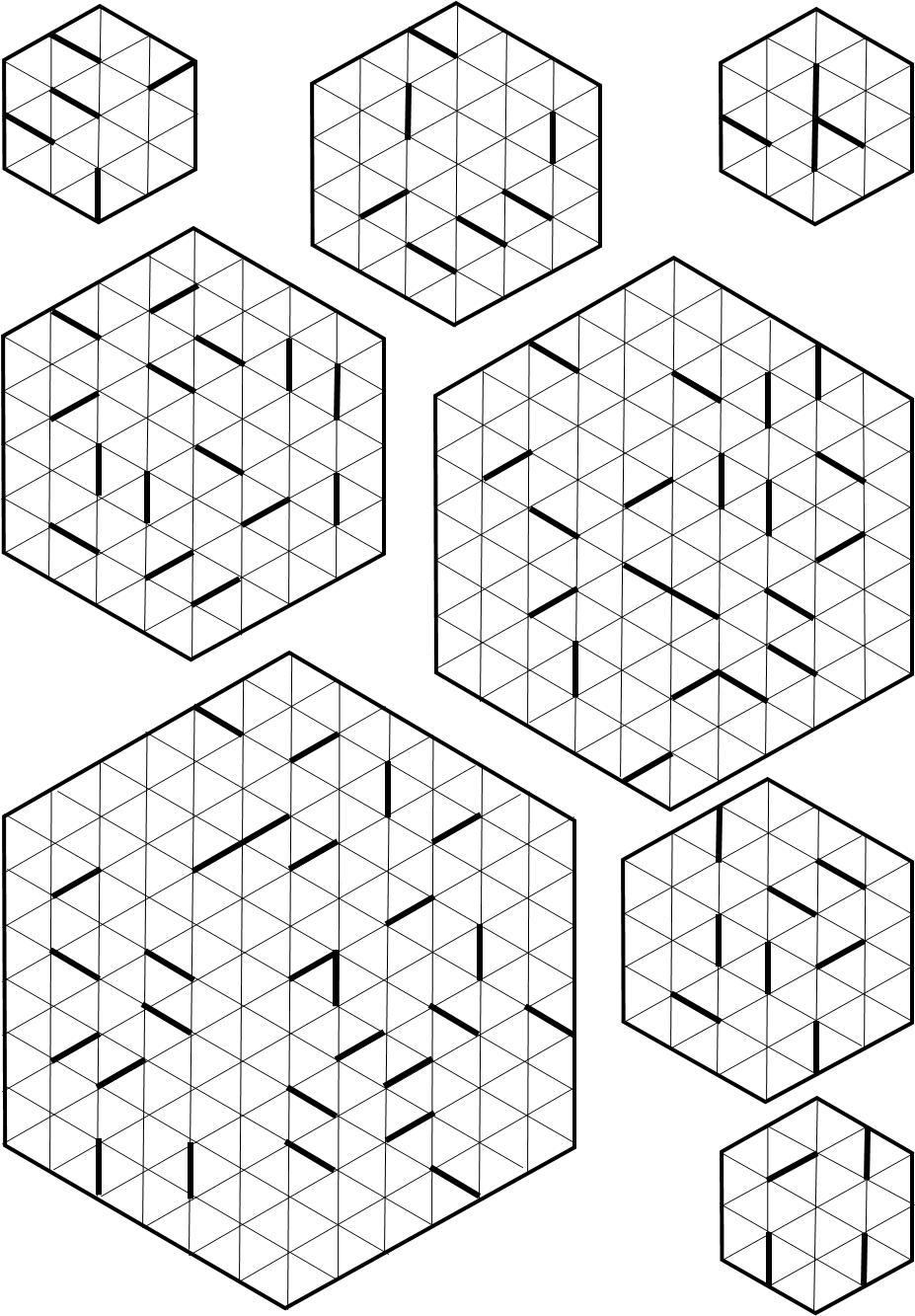
The puzzle appeals to the classical observation that lozenge tilings can be viewed as perspective images of stepped surfaces. As exercise, we invite the reader to solve some of the instances of the puzzle drawn in Fig. 2.
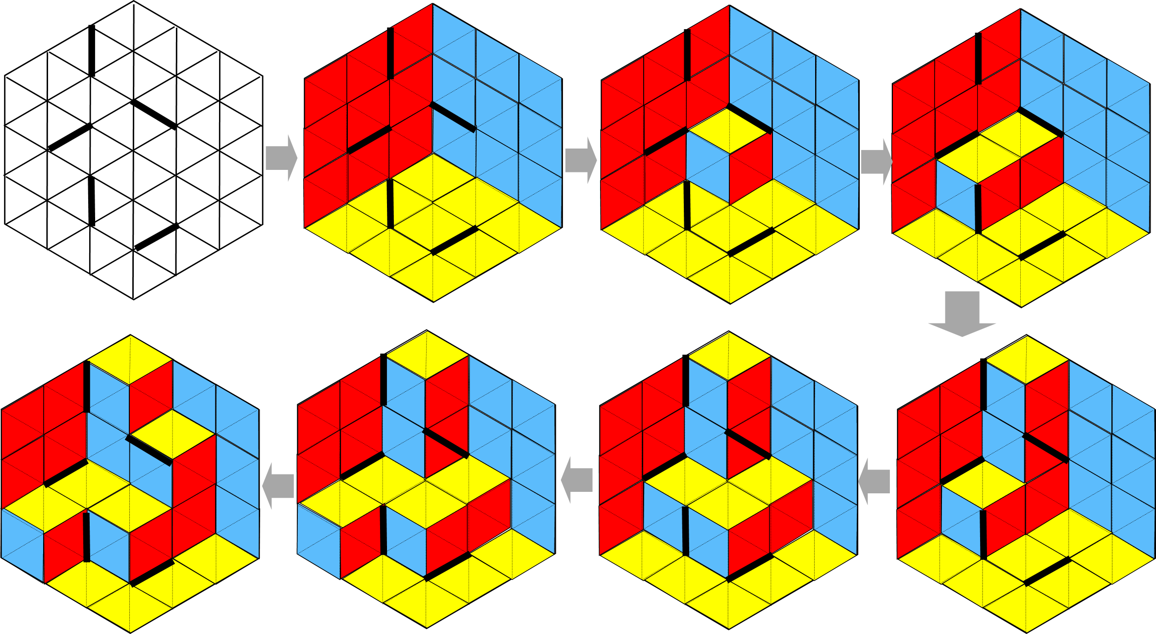
Surprisingly, the Calisson puzzle introduces a saliency constraint (the requirement that lozenges adjacent to a given edge have different orientations) that usual tiling algorithms cannot handle directly. The most classical algorithmic strategy for tiling regions by dominoes or lozenges is to reduce the problem to the computation of a matching. The interest of the Calisson puzzle comes from the fact that this strategy fails, as illustrated in Fig. 6, while the other classical algorithm, Thurston’s algorithm cannot take into account prescribed interior edges. It makes from the computational complexity of the puzzle an interesting question. The first contribution of this paper is a polynomial-time algorithm for solving the Calisson puzzle. We called this algorithm the advancing surface algorithm since its strategy works by adding cubes so that their surface seems to advance from the back of the hexagon to its front. This algorithm is sufficiently simple to be carried out with pencil and paper, and is illustrated in Fig. 3.
Since this algorithm is not a straightforward application of existing results, it naturally raises several questions. Does it extend to arbitrary regions? How does it relate to the classical theory of lozenge tilings? Addressing these questions leads us to the central part of the paper where we revisit and complete the theory and folklore of lozenge tilings from an algorithmic point of view. In Conway and Thurston approach, a lozenge tiling of a simply connected region is lifted to a monotone stepped surface in a three-dimensional cubic lattice. This surface can then be projected back to the plane using a height function defined on the vertices of the triangular grid. In this framework, tiling a region reduces to finding a height function satisfying local constraints.
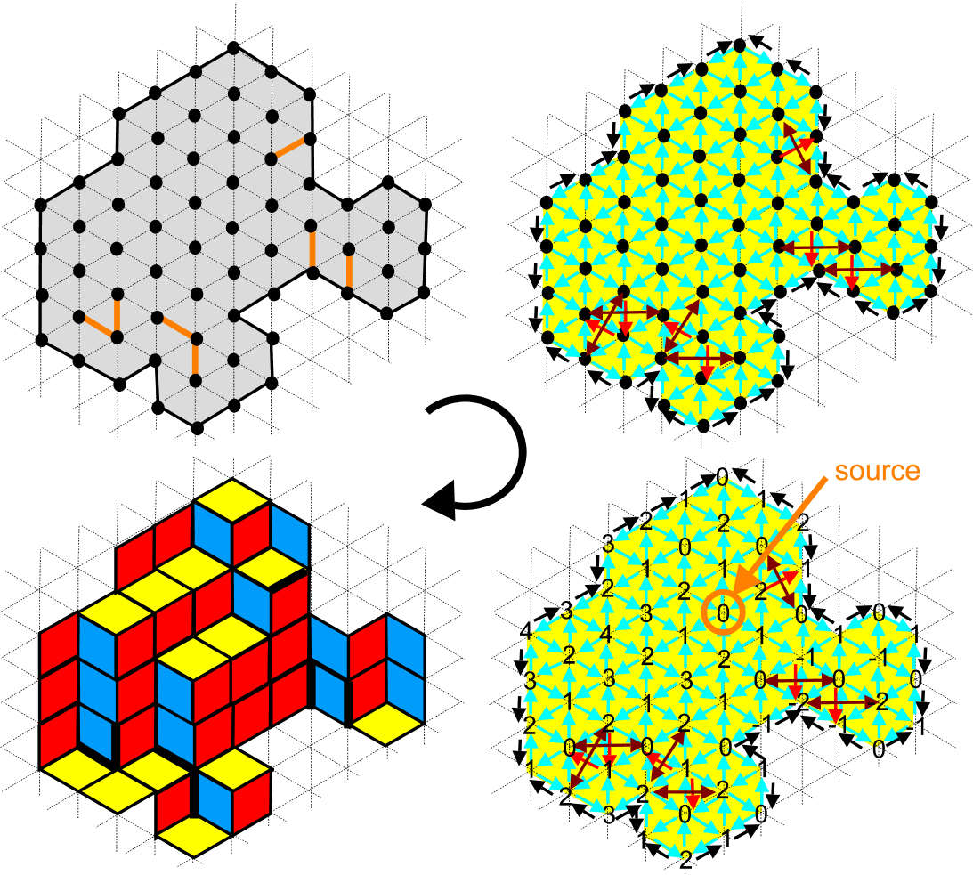
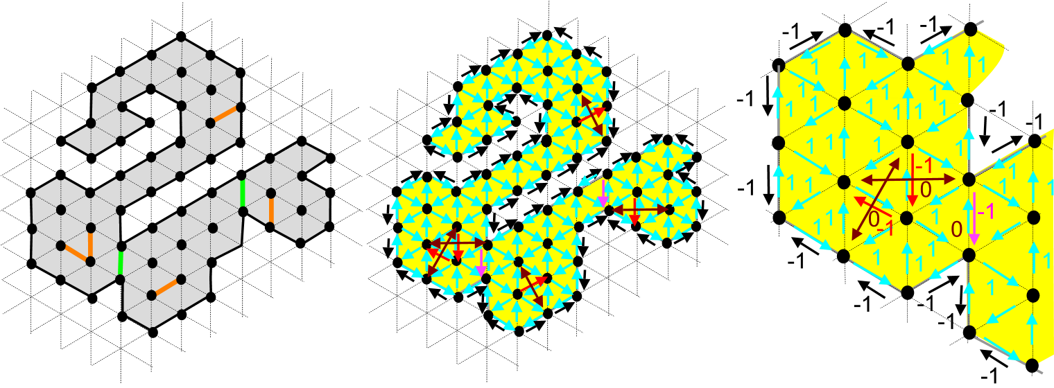
We reformulate Thurston’s theory in the language of directed graphs. Monotone stepped surfaces in the three-dimensional cubic lattice are interpreted as directed cuts (dicuts) in a periodic directed graph whose vertices correspond to unit cubes. Within this framework, height functions naturally arise as solutions of systems of difference constraints. It shows that lozenge tilings can be computed by solving shortest-path problems in weighted directed graphs. With negative weights, the shortest paths algorithm is Bellman–Ford [1]. This original process is illustrated in Fig. 4.
The directed graph overlay introduced in this work constitutes a substantial complement of Thurston’s classical theory of lozenge tilings. It provides a unified and flexible algorithmic framework, allowing one to incorporate interior constraints – such as non-overlapping and saliency constraints – in a simple and systematic way. To the best of our knowledge, such constraints had not previously been integrated explicitly into the height-function framework. This approach makes it possible to solve a wide variety of lozenge tiling problems, several of which are illustrated in Fig. 5. Finally, beyond its theoretical interest, the method has an appealing pedagogical aspect: before understanding the underlying theory, computing a tiling by merely running a shortest-path algorithm, as in Fig. 4, has the flavor of a magic trick, which can surprise and attract the attention of young audiences who are sensitive to recreational mathematics.
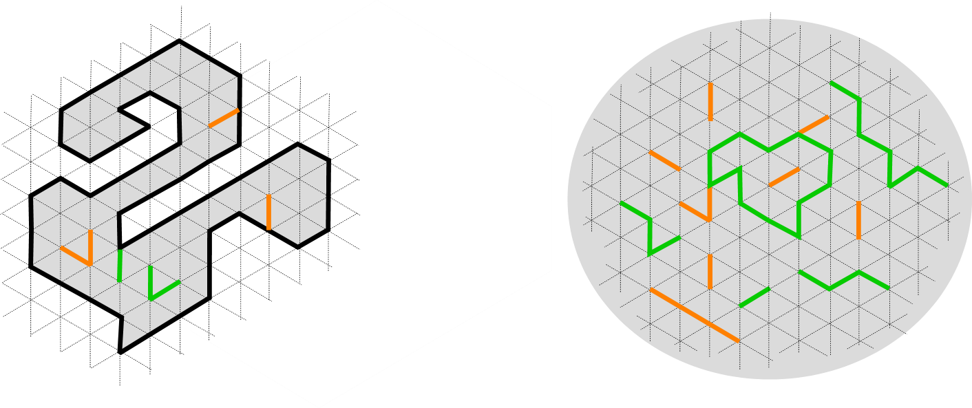
The paper is organized as follows. In Section 2, we present a state of the art of the classical algorithm that can be used for solving the Calisson puzzle and which turn out to fail. In Section 3, we state formaly a generic problem of tilability and present our results. In Section 4, we explain how the lozenges tiling problems can be reduced to systems of difference constraints. This equivalence passes through directed cuts in a periodic directed graph. The algorithms are presented in details in Section 5.
2 Classical Algorithms Fail to Solve the Calisson puzzle
A reasonable idea for solving Calisson puzzles is to use classical techniques from tiling problems. The classical Thurston’s algorithm for determining whether a region is tilable by calissons can take into account neither the interior edges of the instance, nor the saliency constraints. It is therefore not directly able to solve the Calisson puzzles without the kind of complement that we describe in the paper. However, there are other approaches, either used for tilability by dominos or for general combinatorial problems. Three methods are worth examining: -SAT, matching in a bipartite graph and a reduction to Maximum Independent Set.
3-SAT.
The Calisson puzzle is easily expressed as a 3-SAT formula. Consider a variable for each lozenge of the region to be tiled. The variable is equal to if the lozenge is included in the solution’s tiling and otherwise. We have four classes of clauses.
-
-clauses for expressing the condition that all the triangles of the region must be covered by at least one lozenge (for boundary triangles, these are 2-clauses or even 1-clauses).
-
-clauses for avoiding to cover twice a given triangle.
-
-clauses for expressing the non overlapping constraints of the input edges.
-
-clauses for expressing the saliency constraints.
Unfortunatly, this reduction to 3-SAT does not provide a Horn formula and thus it is not known for being solvable in polynomial time.
Matching.
A classic, non-exponential approach to compute tilings by dominoes (lozenges are unions of two adjacent triangles) is to reduce the problem to the computation of a perfect matching in the graph of adjacency of the triangles (see for example [5]). This approach is illustrated in Fig. 6. It allows us to tile the region by taking into account the non overlapping constraints given by the edges of , but not the saliency constraints. Adapting the matching strategy to take into account the saliency constraints does not seem easy.


Maximum Independent Set in an almost perfect graph.
The idea is to consider a dual graph whose nodes are the edges of the triangular grid and where nodes/edges are linked when they belong to a common triangle. In this graph, an independent set of nodes can be seen as a set of lozenges which do not overlap. It reduces the computation of a tiling of a region to the computation of a maximum independent set as done in Fig. 7. The saliency constraint can be taken into account by replacing the forbidden edges by crossed links (green crosses in the second row of Fig. 7). Unfortunatly, this new graph is no more a line perfect graph for which a maximum independent set is known to be computable in polynomial time.
3 Problem Statement and Results
We first provide a general formulation of lozenge tiling problems with optional non overlapping and saliency constraints. We then state the main results of the paper.
3.1 Problem Statement
Regions to which our results apply.
The triangular grid is denoted . We use the letter to denote a region of the triangular grid. Formally, is a simplicial complex whose sets of triangles, edges, and vertices are respectively denoted by , , and . Motivated by the Calisson puzzle, particular attention is paid to regular hexagonal regions. The regular hexagon of size is denoted by .
The results presented in this paper do not require the region to be compact. However, we assume that is simply connected (i.e connected with no holes). In particular, we consider instances where the region is the entire infinite triangular grid, denoted , together with a finite set of input edges. The boundary of is denoted by .
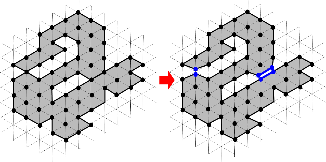
Our results can also be extended to regions whose boundary passes several times through the same vertices or edges. As long as no saliency constraint is imposed on such shared edges, this can be handled by duplicating boundary vertices and edges, as illustrated in Fig. 8. For the sake of simplicity, we omit these cases from the formal statements and proofs.
Edge constraints.
We consider two types of constraints on edges of the triangular grid. The first set, denoted , consists of edges that must not be overlapped by any lozenge. This is the non overlapping constraint. The second set, denoted , consists of edges that must not be overlapped and whose two adjacent lozenges must have distinct orientations. This additional requirement is the saliency constraint.
Generic lozenge tiling problem.
This leads to the following general tiling problem:
Tiling
-
Input: A region and a set of edges of the triangular grid, partitioned into two subsets .
-
Output: A lozenge tiling of the region such that (i) no edge of is overlapped by a lozenge, and (ii) for every edge in , the two adjacent lozenges have different orientations.
A Calisson puzzle with a set of interior saliency constraints corresponds to the instance Tiling.
3.2 Results
We present two algorithmic approaches, both rooted in the three-dimensional interpretation of lozenge tilings as stepped surfaces.
The Advancing Surface Algorithm.
The advancing surface algorithm is illustrated in Figs. 3 and 18 on instances of the Calisson puzzle Tiling. It fills an initially empty cube of size by progressively adding unit cubes, each time adding as few cubes as possible, so as to satisfy the non overlapping and saliency constraints as a simple graph traversal algorithm. It can be easily extended to bounded, simply connected regions of the triangular grid. This extension only requires to add a preprocessing step that computes the minimal and maximal tilings (for instance by running classical Thurston’s algorithm). The advancing surface algorithm then progressively adds unit cubes in the volume between these two extremal tilings. The algorithm and its analysis are detailed in Subsection 5.2.
Theorem 1.
The advancing surface algorithm solves Tiling for a bounded, simply connected region in running time .
In the special case of the Calisson puzzle, the region is the hexagon . Then the two extremal tilings are straightforward (the projections of the surface of an empty and a full cube).
Corollary 2.
The advancing surface algorithm solves Calisson puzzle instances
Tiling
with running time .
Reduction of Tiling to a System of Difference Constraints.
The main contribution of this paper is the completion of Thurston’s theory of lozenge tilings with a graph-theoretical layer. This additional structure allows us to translate the generic tiling problem Tiling into an equivalent system of difference constraints. This system is induced by a weighted directed graph, denoted and defined as follows:
Construction of the DC graph
Some notations: An oriented edge of the triangular grid is said to be positive if it points in the time direction of , , or o’clock, and negative if it points in the time direction of , , or o’clock.
We also introduce lateral edges, which complement the edges of the triangular grid. Given an edge of the triangular grid, let and be the two vertices adjacent to both and . The lateral edges associated with are the two oriented edges and .
Construction of the weighted directed graph
:
The construction can be followed in Fig. 9.
The vertex set of is the set of the vertices of the region .
Its directed edges are defined as follows:
-
Every positively oriented edge contained in is assigned weight .
-
For every edge in , the negatively oriented version of is assigned weight . These edges encode the non-overlapping constraints.
-
For every edge , the pair of lateral edges associated with is assigned weight . These edges encode the saliency constraints.
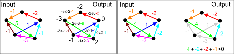
A system of difference constraints induced by a weighted directed graph is the assignation problem of a value to each vertex such that, for every directed edge with weight , the inequality is satisfied (see Fig. 10 or reference CLRS [2] section 24.4).
We claim that the tiling instance Tiling is equivalent to the system of difference constraints induced by .
Theorem 3.
There is a one-to-one correspondence between the tiling which are solutions of Tiling and integer-valued functions satisfying the system of difference constraints induced by , up to an additive constant.
The tiling is obtained from the integer-valued function by linking the adjacent vertices of whose value differ from (as illustrated in Fig. 4).
Classically, systems of difference constraints are solved by shortest-path algorithms such as Bellman–Ford [2]. If the graph contains a directed cycle of strictly negative total weight, then the system has no feasible solution. Otherwise, shortest-path distances from an arbitrary source yield a valid solution of the constraints.
This dichotomy is illustrated in Fig. 11.

As a direct consequence of Theorem 3, we obtain the following corollary.
Corollary 4.
For any finite simply connected region , the tiling problem Tiling can be solved in time by applying the Bellman–Ford algorithm to the directed graph .
We conclude this section by considering the decision problem of tiling the entire triangular grid with a finite set of constraints and .
Corollary 5.
Let and be finite sets of edges. The feasibility of Tiling can be decided by solving a finite system of difference constraints derived from , in time .
Due to the absence of boundary conditions and the infinite number of tiles, this last problem cannot be addressed by classical approaches such as matching-based methods, Thurston’s original algorithm, SAT encodings, or maximum independent set formulations. The corollary 5 illustrates that the difference constraints formulation induced by is not a mere technical rewriting of Thurston’s theory, but rather an essential complement that clarifies the algorithmic theory of lozenge tilings and enables the solution of tiling problems beyond the reach of standard methods. Due to lack of space, we omit its proof and report the reader to the full Arxiv version of the paper.
4 Why it Works
The goal of this section is to prove Theorem 3 by showing that solving the generic tiling problem Tiling is equivalent to solving the system of difference constraints induced by the weighted directed graph .
This equivalence is obtained through a sequence of transformations that can be summarized as Each transformation is the purpose of a dedicated subsection, and an additional subsection is devoted to the encoding of the non-overlapping and saliency constraints. Thurston’s original approach follows the shorter path which is sufficient for simply connected regions without interior constraints. Our contribution is to make explicit the intermediate graph-theoretic structure of directed cuts, which provides a complete and uniform framework before passing to height functions and difference constraints. This additional layer makes it possible to incorporate interior constraints and to rely on classical algorithmic tools from Theoretical Computer Science.
4.1 Notations
The Grids , , and the Projection .
The primary unit cube is . The cubes of the cubic grid are denoted , with (see Fig. 12). The sets of cubes, faces, edges, and vertices of the cubic grid are respectively denoted , , , and . Throughout the paper, we follow the convention that a superscript indicates the dimension of the objects in the corresponding set.
The infinite triangular grid is obtained by projecting the edges of using a map . More precisely, denotes the projection of the three-dimensional space onto a plane of equation , along the direction . The plane is naturally decomposed into a simplicial complex consisting of triangles, edges, and vertices.
Any vertex of is incident to six edges. Their directions are given by , , , and their opposites. Rather than using two-dimensional coordinates in the plane , we use homogeneous coordinates: a point of is represented as with . Clearly, for any . Adding such a constant changes the height in the direction without affecting the projection. This notion of height was introduced by Thurston. The height of is simply .
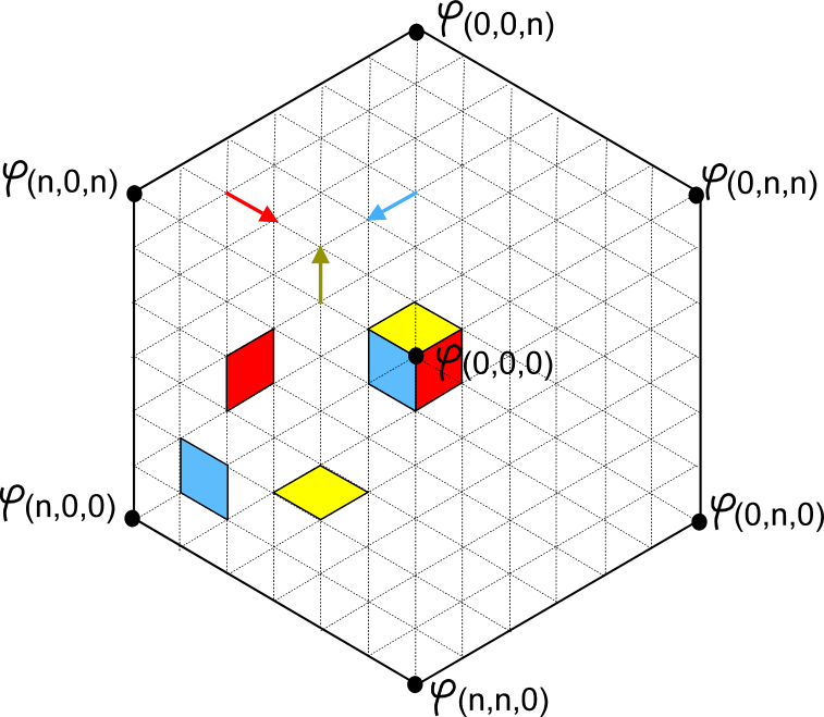
The Lozenges.
Our two-dimensional tiles are lozenges. A lozenge is defined as the projection under of a two-dimensional face of the cubic grid . Since the faces of have three possible orientations, there are exactly three types of lozenges. Blue, red, and yellow lozenges are the projections of square faces with normal directions , , and .
4.2 From Tilings to Roofs (Thurston’s Theorem)
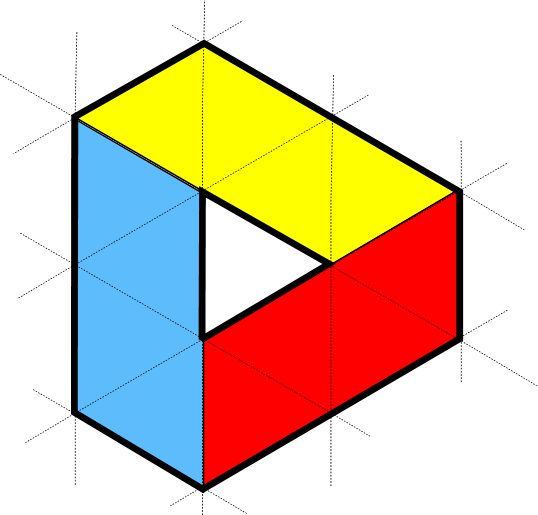
William Thurston showed that any lozenge tiling of a simply connected region can be lifted through to a monotone stepped surface of the cubic grid , where monotonicity is considered with respect to the direction . This surface is unique up to translations in the direction. By fixing the height of a single point, the lifting is therefore uniquely defined. In [9, 8], this surface is called the roof of the tiling .
Theorem 6 (Thurston).
Any lozenge tiling of a simply connected region of the triangular grid can be lifted to a surface of the cubical -complex, denoted and called the roof of , such that the projections of the square faces of the roof are exactly the lozenges of .
Moreover, the height of a vertex is defined as the value of the unique point in that belongs to the roof . This height is defined up to an additive constant, but height differences are unambiguous and play a central role in what follows.
4.3 From Roofs to Directed Cuts
At this point, we depart from the standard geometric viewpoint introduced by Thurston to adopt a graph Theoretical Computer Science framework (directed cuts and difference constraints systems) that is best suited to address the algorithmic questions arising in the computation of lozenge tilings with local constraints.
The Ascendant Graph of Cubes and Its Projection.
With our notation, each cube of is identified with its base point , yielding a natural one-to-one correspondence between and . We define as the set of cubes whose base points project into the region , that is, such that . Equivalently, consists of infinite stacks of cubes above the vertices in the direction .
We endow with a directed graph structure, called the ascendant graph and denoted . There is a directed edge in if and only if the following two conditions hold:
-
(a)
the cube is one of the three cubes , , or . In other words, edges of go from a cube to one of its three face-adjacent cubes of height exactly one unit higher.
-
(b)
The projection of this edge by , , is an edge of the triangular grid belonging to the region, that is, .
When the boundary of the region folds back onto itself, Condition (b) prevents the introduction of spurious edges. By construction, the edges of the ascendant graph correspond to square faces of the cubic grid whose projections by are either entirely contained in or overlap boundary edges of .
Remark 7.
The projection of the adjacent square face/edge of from to is precisely the lozenge overlapping the edge of the triangular grid. The same remark holds for the two other coordinate directions.
The ascendant graph is acyclic, hence a directed acyclic graph (DAG). Moreover, it is invariant under translations by vectors of the form with , and therefore admits a -periodic structure. This periodicity is essential and will be exploited later.
Roofs as Directed Cuts of the Ascendant Graph.
We now return to the roof associated with a lozenge tiling of a simply connected region and interpret it as a directed cut of the ascendant graph .
Each square face of the roof is adjacent to a pair of cubes and , where equals one of , , or . Since the projection of this square face by lies in the region , both cubes belong to and therefore define an edge of . It follows that the square faces of the roof correspond exactly to a subset of edges of the ascendant graph. This subset has an important property.
We now introduce the notion of a directed cut (or dicut) of a directed graph. A dicut is a partition of the vertex set into two non empty subsets that we denote and such that all edges crossing the cut are directed from to . The difference between a simple cut and a dicut is illustrated in Fig. 14.

One of the properties that we use in the following is that a directed path in a directed graph cannot be cut twice by a dicut.
The roof of the tiling being a monotone surface, it provides a partition of the cubes of which are above and below it. This partition is a dicut of .
Claim 8.
The roof of a tiling of a simply connected region defines a dicut of the ascendant graph .
At this stage, the correspondence is only one-way. While the roof of a tiling of always induces a directed cut of the ascendant graph , the converse is not true in general: there exist dicuts of whose projections (the projections of the square faces separating the two sides of the cut) do not form a valid tiling of the region , because some projected lozenges may overlap boundary edges of or violate interior constraints.
From the algorithmic perspective of solving an instance of Tiling, the central question therefore becomes the following: under which conditions does the projection of a dicut of the ascendant graph yield a valid tiling of the region satisfying the non overlapping and saliency constraints encoded by and ?
4.4 Encoding the Local Constraints by Unbreakable Edges
We arrive at the step where the dicut perspective is essential. We express the constraints that a dicut must satisfy for providing a valid solution of Tiling by introducing the notion of unbreakable edges. Certain edges of the ascendant graph must not be crossed by a dicut, because cutting them would produce projected lozenges that violate the tiling constraints. We now explain how the non overlapping and saliency constraints translate into unbreakable edges in .
Non Overlapping Constraints.
The first type of constraint enforces that no lozenge overlaps either a boundary edge of or an interior edge belonging to . Consider, for instance, an edge of the triangular grid between the vertices and that must not be overlapped by a lozenge. By Remark 7, the lozenge overlapping this edge is exactly the projection of the square face separating the cubes and .
Therefore, forbidding this overlap is equivalent to requiring that the directed edge of from to does not belong to the dicut. The same restriction applies to all translated pairs and for any . In other words, all directed edges between these pairs of cubes are declared unbreakable. Conversely, if a directed cut does not cut any of these unbreakable edges, then the corresponding lozenge overlapping the edge cannot appear in the projection. Equivalent claims hold for the two other directions. It shows that by declaring unbreakable some pairs of cubes and for any , we exactly encode the non overlapping constraints.
Saliency Constraints.
We now consider the saliency constraints imposed by the edges of . Assume that the edge between the vertices and belongs to . The saliency constraint requires that the two lozenges adjacent to have distinct orientations.
To encode this condition in the ascendant graph, we introduce four families of cubes for each integer :
as illustrated in Fig. 15. Each of these cubes has a face whose projection is a lozenge adjacent to or overlapping the edge .
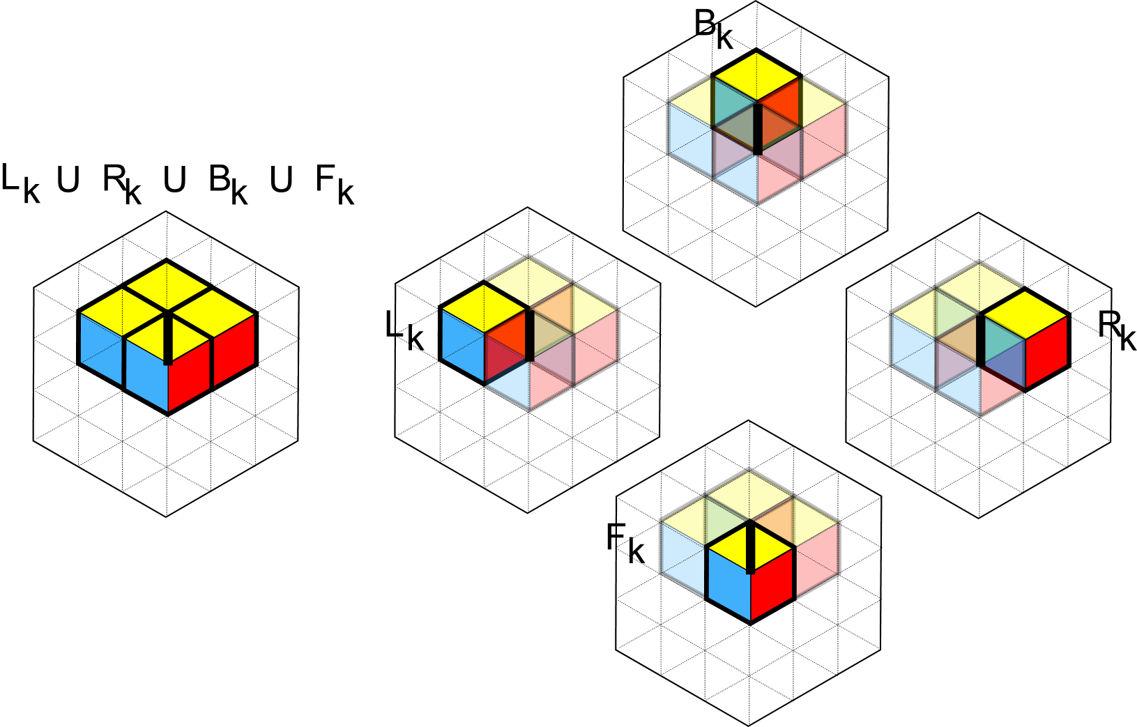
With this notation, the non overlapping constraint on is expressed by declaring the edge from to unbreakable. We now show how the saliency constraint itself can be enforced. The ascendant graph contains the following chain of cubes: Any directed cut must intersect this infinite periodic chain at least once, otherwise one side of the cut would be empty. Several cutting patterns are possible, as shown in Fig. 16.
Cutting the two edges and satisfies the saliency constraint (Case 1 in Fig. 16). In contrast, cutting together with (Case 2), or symmetrically cutting together with (Case ), produces two adjacent lozenges of the same orientation and therefore violates the saliency constraint. Cutting both edges and is valid (Case 3). Finally, cutting violates the non overlapping constraint on .
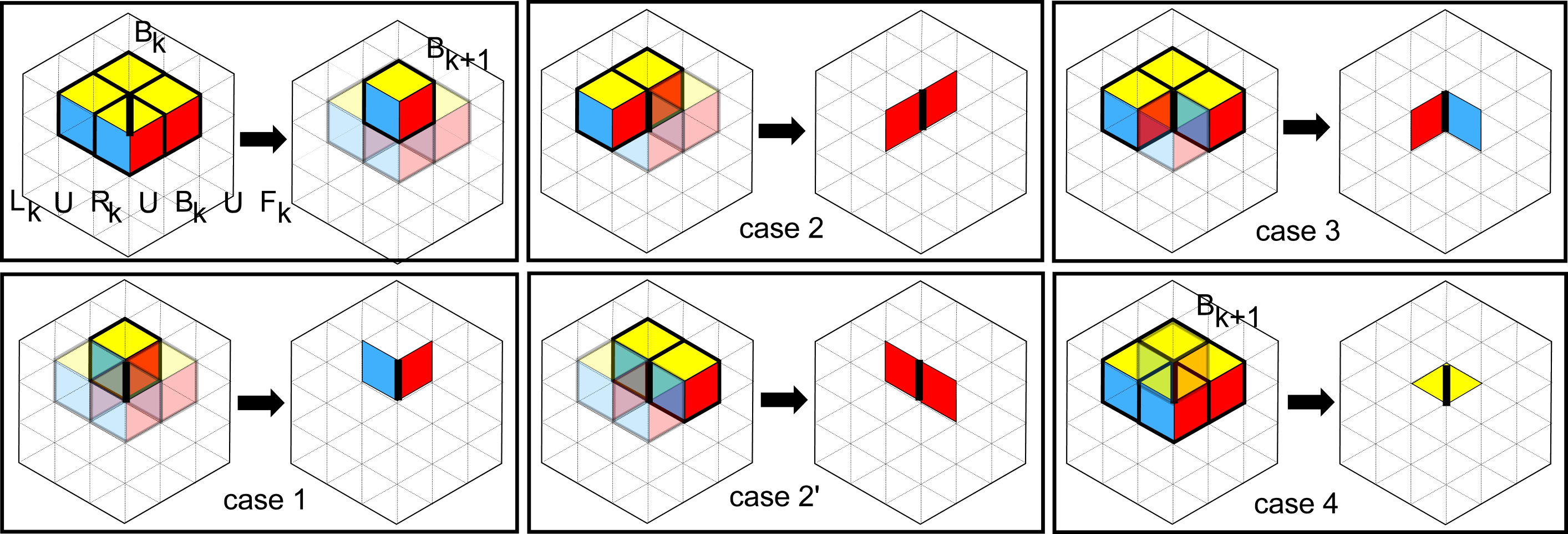
The conclusion is that the saliency constraint on the edge is satisfied if and only if the two cubes and lie on the same side of the dicut. Equivalently, for every , the pair must not be separated by the dicut. Thus, the saliency constraint is enforced by declaring an unbreakable edge between and for all .
The Enhanced Ascendant Graph .
A simple way to enforce that two vertices and of a directed graph belong to the same side of any dicut is to add a pair of opposite directed edges: one from to and one from to . Indeed, no dicut can separate and without cutting at least one of these edges in a wrong direction.
This observation provides a simple mechanism for incorporating non overlapping and saliency constraints into the ascendant graph. We denote by the enhanced ascendant graph, obtained from by adding, for every unbreakable constraint induced by , , and , a pair of edges in opposite directions between the corresponding cubes.
We can now state the central correspondence between tilings and dicuts.
Proposition 9.
A tiling is a solution of the generic tiling problem Tiling if and only if is the projection by of a dicut of the enhanced ascendant graph .
Moreover, the corresponding dicut is unique up to a global translation along the vector , reflecting the classical height-shift ambiguity.
The proof of Theorem 9 is simply obtained by merging the previous arguments. The main idea is the translation of the non overlapping and saliency constraints into the unbreakable edges added in the enhanced ascendant graph . The detailed proof can be found in the full version available on ArXiv.
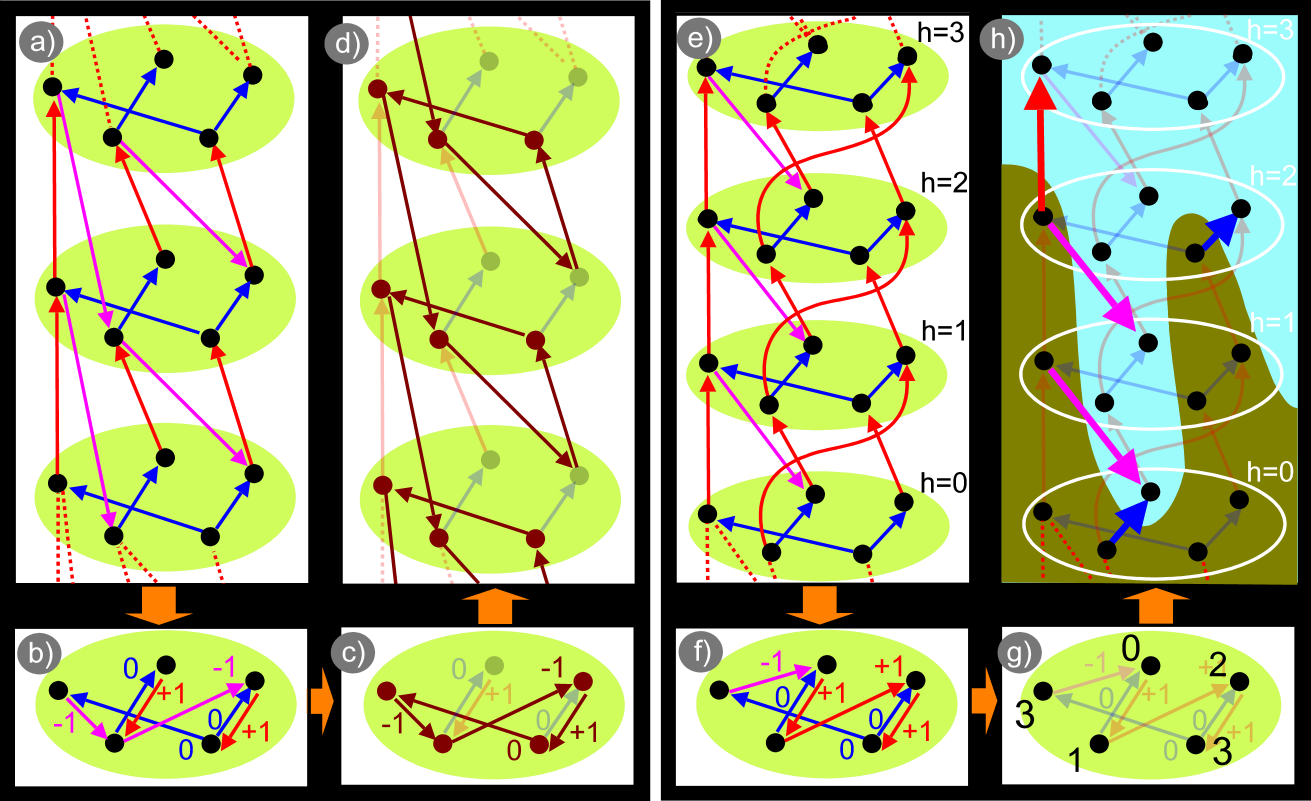
The goal of the next steps is to transform the problem of computing a dicut in the periodic graph into a system of difference constraints. This type of reduction is not specific to the graph : it applies more generally to -periodic directed graphs. Since a full general treatment is beyond the scope of this paper, we only illustrate the mechanism in Fig. 17, using -periodic graphs different from . The purpose of this illustration is to provide intuition for why dicuts in -periodic graphs can be characterized and computed via systems of difference constraints.
4.5 From Dicuts to Height Functions
Any dicut of the enhanced ascendant graph can be characterized by the heights of the highest cubes belonging to the part of the cut. Equivalently, a dicut induces an integer-valued function , defined on the vertices of the triangular grid, where is the maximum height of a cube of and that lies below the cut (with the association cube / point that we use, the height of the cube is the height of the point ).
The function is defined up to an additive constant, reflecting the invariance of under translation by the vector . Up to this global shift, coincides with Thurston’s classical height function associated with lozenge tilings.
4.6 From Height Functions to Difference Constraints
Each directed edge of the enhanced ascendant graph induces a local constraint on the height function . Here (resp. ) is a cube projecting onto a vertex (resp. ) of the region . We denote by the fixed height increment associated with this edge, namely
Let be the highest cube based in that lies below the cut. By definition, its height is . By the -periodicity of the graph , the directed edge appears at all vertical levels. In particular, there exists a cube based in a point of such that is an edge of . Since this edge has height increment , the cube has height .
As lies below the cut, we must have , or equivalently,
Thus, each directed edge of yields a difference constraint on the height function .
In the enhanced ascendant graph , the value of depends only on the type of the edge. There are three types of edges:
-
1.
The original ascendant edges of , which go from a cube to one of its three upper adjacent cubes. These edges increase the height by and therefore have weight .
-
2.
The descending edges added to encode non overlapping constraints through unbreakable edges (arising from and from ). These edges go from to , , or , and decrease the height by . Their weight is .
-
3.
The unbreakable edges encoding saliency constraints, which connect pairs of cubes at the same height (such as the cubes and ). These edges have weight .
Collecting all such inequalities yields a system of difference constraints whose variables are the values for . In Section 2, we have denoted by the weighted directed graph encoding these constraints. This last step ends the sequence of transformations of the generic tiling problem Tiling and proves Theorem 3.
Theorem 3.
[Restated, see original statement.]
There is a one-to-one correspondence between the tiling which are solutions of Tiling and integer-valued functions satisfying the system of difference constraints induced by , up to an additive constant.
Absorbing Cycles and Feasibility.
A classical result on systems of difference constraints states that such a system is feasible if and only if the associated weighted directed graph contains no cycle of strictly negative total weight. These two cases are illustrated in Fig. 11. It shows the next corollary of Theorem 3.
Corollary 10.
A tiling instance Tiling admits a solution if and only if the graph has no cycle of strictly negative weight.
When there is no cycle of strictly negative weight, a feasible height function can be computed using classical shortest-path algorithms for graphs with possibly negative weights, such as the Bellman-Ford algorithm [1]. The resulting height function directly defines a dicut of and therefore a valid tiling of the region . It provides the first algorithm that we now discuss with its variants.
5 Algorithms
We now discuss the algorithms that can be used to solve the generic tiling problem Tiling before concluding the section with the special case where the underlying region is the infinite triangular grid subject to finitely many local constraints.
5.1 Bellman-Ford
The Bellman–Ford algorithm is the standard method for solving systems of difference constraints [1]. Given a weighted directed graph, it detects the presence of a cycle of strictly negative total weight, and otherwise computes a set of distances satisfying all constraints. Its time complexity is for a graph with vertex set and edge set .
A direct strategy for solving Tiling consists of first constructing the weighted directed graph , which can be done in linear time with respect to the size of the region, and then applying the Bellman–Ford algorithm to the resulting system of difference constraints. This approach is illustrated in Figs. 3 and 4.
In the graph , the vertex set is , and the number of edges is linear in . Therefore, running Bellman–Ford on requires time or equivalently time. In particular, for the Calisson puzzle Tiling, where , the Bellman–Ford approach runs in time .
5.2 The Advancing Surface Algorithm
Unlike the advancing surface algorithm, this new algorithm does not compute a height function on the vertices of the region. Instead, it works directly in the graph of cubes by constructing a dicut of the enhanced ascendant graph .
The key idea is that it is not necessary to consider the full infinite graph . One can restrict attention to a finite domain delimited by two extremal dicuts and then compute a solution by a graph traversal procedure.
First step: Lower and Upper Dicuts.
As in Thurston’s algorithm, we first examine the boundary of the region . If the directed boundary cycles has nonzero total weight, then is not tilable and we stop. We therefore assume that the boundary cycle has total weight zero.
We temporarily ignore the interior constraints and work in the cube graph . The boundary cycle of can be lifted to a directed cycle in this graph. By periodicity, this yields an infinite stack of directed cycles, each translated from the previous one by the vector . If the region is tilable, the graph admits a dicut, and each cycle of this stack lies entirely either in the bottom or in the top part of the cut. Consequently, there exists a pair of consecutive cycles and such that lies in the bottom part and in the top part of the dicut. Then all cubes that can reach a cube of by a directed path belong to the lower part of a new dicut, which we call the lower cut. Dually, all cubes reachable from a cube of belong to the upper part of a second new dicut, called the upper cut. Any dicut of separating and must lie between these two extremal cuts.
The first step of the algorithm therefore consists in computing the lower and upper dicuts of using Thurston’s algorithm. Either this step determines that is not tilable, or it provides the two extremal dicuts.

Second step: Incorporating Interior Constraints.
Assuming the first step succeeds, we now incorporate the interior constraints given by and . These constraints introduce additional directed edges in the enhanced graph , which may create new predecessors for cubes in the lower cut.
The second step consists of a graph traversal starting from the lower cut: we iteratively add to the lower part of the lower dicut all cubes that have a directed edge leading to an already known cube of the lower part.
If during this process a cube belonging to the top part of the upper cut is added, then no dicut separating and exists. In this case, the instance Tiling is not feasible. Otherwise the growth of the bottom part of the lower dicut eventually ends when it remains no predecessor to add, providing a dicut of the graph and thus a tiling solution of Tiling .
Complexity.
The time complexity of the first step is that of Thurston’s algorithm. The second step visits only cubes lying between the lower and upper dicuts of . The vertical distance between these two cuts is bounded by the length of the boundary, namely . Therefore, the number of cubes in this intermediate region is at most , which bounds the running time of the second step.
Overall, the advancing surface algorithm runs in time .
In the particular case of the Calisson puzzle Tiling, the lower and upper cuts are trivial: they correspond respectively to the empty and full cube. Since and , the advancing surface algorithm runs in time .
With a Pencil and a Rubber.
Although the mathematical framework underlying the advancing surface algorithm is nontrivial, its implementation in the context of the Calisson puzzle is remarkably simple. Using only a pencil, an eraser, and a three-dimensional intuition, one can simulate on the paper the successive additions of cubes. The previous analysis guarantees that this naive-looking procedure never misses a solution when one exists. Figure 18 illustrates several steps of the algorithm applied to the largest instance of Fig. 2.
Future Works
A natural direction for future work is to investigate whether the graph and difference constraints overlay introduced in this paper can be extended to other tiling problems that admit a height-function formulation. Is this approach specific to lozenge tilings or does it apply to a broader class of planar tilings whose configurations can be encoded by monotone surfaces?
References
- [1] Richard Bellman. On a routing problem. Quarterly of Applied Mathematics, 16:87–90, 1958.
- [2] Thomas H. Cormen, Charles E. Leiserson, Ronald L. Rivest, and Clifford Stein. Introduction to Algorithms. The MIT Press, 2nd edition, 2001. URL: https://en.wikipedia.org/wiki/Introduction_to_Algorithms.
- [3] Jean-Marie Favreau, Yan Gerard, Pascal Lafourcade, and Léo Robert. The calissons puzzle, 2023. doi:10.48550/arXiv.2307.02475.
- [4] Jean-Marie Favreau, Yan Gerard, Pascal Lafourcade, and Léo Robert. Lozenge tiling by computing distances, 2026. arXiv:2603.02476.
- [5] Claire Kenyon and Eric Rémila. Perfect matchings in the triangular lattice. Discrete Mathematics, 152(1):191–210, 1996. doi:10.1016/0012-365X(94)00304-2.
- [6] Olivier Longuet. Le jeu du calisson, 2022. [accessed in January 2026]. URL: https://mathix.org/calisson/blog/.
- [7] Arnaud Durand Martial Tarizzo. Speedy calisson game, 2024. [accessed in January 2026]. URL: https://martialtarizzo.github.io/Calisson-Game/index.en.html.
- [8] William P. Thurston. Conway’s tiling groups. The American Mathematical Monthly, 97(8):757–773, 1990. doi:10.1080/00029890.1990.11995660.
- [9] William P. Thurston. Groups, tilings, and finite state automata. Summer 1989 AMS Colloquium lectures, 1990.