Shortest Paths in Geodesic Unit-Disk Graphs

Abstract
Let be a set of points in a polygon with vertices. The geodesic unit-disk graph induced by has vertex set and contains an edge between two vertices whenever their geodesic distance in is at most one. In the weighted version, each edge is assigned weight equal to the geodesic distance between its endpoints; in the unweighted version, every edge has weight . Given a source point , we study the problem of computing shortest paths from to all vertices of . To the best of our knowledge, this problem has not been investigated previously. A naive approach constructs explicitly and then applies a standard shortest path algorithm for general graphs, but this requires quadratic time in the worst case, since may contain edges. In this paper, we give the first subquadratic-time algorithms for this problem. For the weighted case, when is a simple polygon, we obtain an -time algorithm. For the unweighted case, we provide an -time algorithm for simple polygons, and an -time algorithm for polygons with holes.
Keywords and phrases:
unit-disk graph, geodesic distance, shortest paths, geodesic Voronoi diagrams, range emptiness queries, dynamic data structuresCopyright and License:
![[Uncaptioned image]](x1.png) © Bruce W. Brewer and Haitao Wang; licensed under Creative Commons License CC-BY 4.0
© Bruce W. Brewer and Haitao Wang; licensed under Creative Commons License CC-BY 4.0
2012 ACM Subject Classification:
Theory of computation Computational geometry ; Theory of computation Design and analysis of algorithmsEditors:
Hee-Kap Ahn, Michael Hoffmann, and Amir NayyeriSeries and Publisher:
 Leibniz International Proceedings in Informatics, Schloss Dagstuhl – Leibniz-Zentrum für Informatik
1 Introduction
Let be a set of points in the plane. The unit-disk graph induced by has vertex set and contains an edge between two vertices if their Euclidean distance is at most one. Equivalently, the unit-disk graph is the intersection graph of the set of congruent disks of radius centered at the points of : each disk corresponds to a vertex, and two disks are adjacent precisely when they intersect. Unit-disk graphs are extensively studied in computational geometry due to their rich geometric structure and numerous applications [12]. One motivation arises from wireless ad-hoc networks. Here, each point of models a device capable of transmitting and receiving wireless signals within a fixed range, which we normalize to one. Thus, two devices can communicate directly exactly when they are connected by an edge in the corresponding unit-disk graph. Many fundamental algorithmic tasks for wireless networks reduce to classical graph problems on unit-disk graphs, such as coloring, independent set, and dominating set [12]. A central question is how to route a message between two devices and . If and are not within communication range, then the message must be relayed via intermediate devices. In graph terms, the message must follow an - path in the unit-disk graph, and ideally one of minimum length. For this reason, the shortest path problem in unit-disk graphs plays a key role in both theory and applications.
Another natural application of unit-disk graphs arises in motion planning with recharging/refueling. Suppose a vehicle (for example, a delivery drone) must travel from a start point to a target point , but lacks sufficient battery capacity to traverse this distance directly. Instead, it may need to stop at intermediate charging stations. Consider the graph whose vertices represent charging stations and where two stations are connected by an edge if the vehicle can travel between them on a full charge. After scaling the maximum travel distance on a full charge to one, this graph is precisely a unit-disk graph. Thus, the motion planning problem reduces to finding a shortest - path in the unit-disk graph.
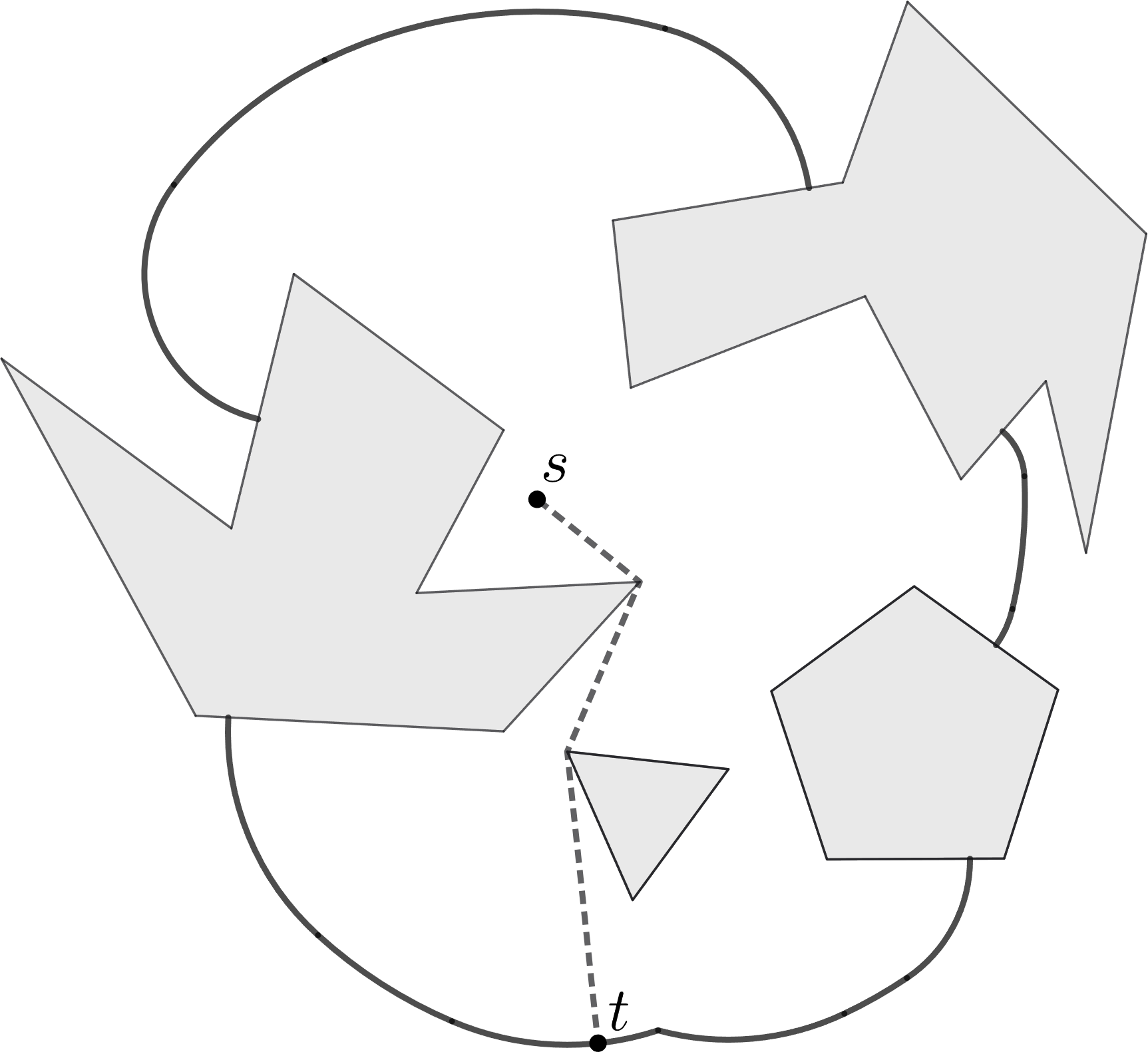
Now consider the above applications in the presence of obstacles that must be avoided. In wireless ad-hoc networks, an obstacle may prevent a signal from traveling directly between two devices, forcing it to bend around buildings or terrain features. In the motion planning scenario, obstacles may correspond to physical barriers or restricted regions. In such environments, Euclidean distance no longer reflects the true travel cost between two points. Instead, the relevant distance is the geodesic distance, i.e., the length of a shortest obstacle-avoiding path between two points. Figure 1 illustrates a “geodesic unit disk”.
Problem definition.
Motivated by these applications, we study geodesic unit-disk graphs, defined as follows. Let be a polygonal domain with holes and a total of vertices in the plane. Thus, is a closed, multiply connected region whose boundary consists of disjoint polygonal cycles. The holes of , together with the region outside , are referred to as obstacles. For any two points in , their geodesic distance is the length of a shortest path between them in . Let be a set of points (also called sites) contained in . The geodesic unit-disk graph induced by has vertex set and contains an edge between two sites whenever their geodesic distance is at most one. In the unweighted case, every edge of has weight ; in the weighted case, the weight of an edge is the geodesic distance between its endpoints. The appropriate choice of model depends on the application. Given a source site , we consider the single-source shortest-path (SSSP) problem in : for a given polygonal domain , site set , and source , compute shortest paths in from to all other vertices. To the best of our knowledge, this problem has not been studied previously.
Related work.
As discussed above, problems on Euclidean unit-disk graphs (i.e., when is given in the plane without obstacles) are well studied [12]. For the unweighted case, Cabello and Jejčič [8] gave an -time algorithm for the SSSP problem, matching an lower bound [8]. Chan and Skrepetos [9] later obtained an -time algorithm under the assumption that the points are presorted by - and -coordinates.
For the weighted case, Roditty and Segal [28] obtained an -time algorithm for any . Cabello and Jejčič [8] improved this to time. Their runtime has since been reduced due to improvements in dynamic bichromatic closest-pair structures, first by Kaplan, Mulzer, Roditty, Seiferth, and Sharir [20] and then by Liu [23]. Most recently, Wang and Xue [29] proposed a new algorithm that avoids dynamic bichromatic closest-pair structures, and their algorithm runs in time; Brewer and Wang [7] further improved the time to by refining a key bottleneck subproblem.
1.1 Our results
A straightforward approach is to construct explicitly and then run a standard SSSP algorithm. However, may contain edges, leading to quadratic time in the worst case. In this paper, we present three subquadratic-time algorithms for three problem variants.
-
1.
For the weighted case, when is a simple polygon, we obtain an -time algorithm. When applied to the Euclidean setting by taking (i.e., is the entire plane), our runtime is only roughly a logarithmic factor slower than the current best bound of [29, 7]. The Euclidean algorithms in [29, 7] rely crucially on a grid decomposition of the plane, a technique that does not extend naturally to the polygon setting since a grid cell may be fragmented into multiple disconnected components by the boundary of . We therefore use a different algorithmic strategy.
-
2.
For the unweighted case in a simple polygon, we give an -time algorithm. Applied to the Euclidean setting, this matches the lower bound [8].
-
3.
When has holes, the problem becomes substantially more challenging. For the unweighted case in this setting, we develop an -time algorithm.
Our techniques involve solving two subproblems that may be interesting in their own rights. Indeed, solving these problems is one of the major contributions of this paper.
Subproblem 1: Deletion-only geodesic unit-disk range emptiness queries.
In this problem, we preprocess a set of points inside a simple polygon of vertices to support two operations: (1) given a query point , determine whether there exists a point whose geodesic distance to is at most , and if so return such a point; and (2) delete a point from . We refer to the first operation as a geodesic unit-disk range emptiness (GUDRE) query.
Using the dynamic randomized nearest neighbor data structure of Agarwal, Arge, and Staals [1], each deletion can be supported in expected amortized time, and each GUDRE query can be answered in time. In the Euclidean case (i.e., when is the entire plane), one can preprocess in time and support both queries and deletions in time [14, 30].
We obtain the following result. After an -time global preprocessing step for , we can, for any given set of points in , build a data structure in time such that deletions take amortized time and GUDRE queries take time. Our result is remarkable in three aspects. First, compared to applying [1], our result improves deletion time by a factor of and improves query time by a factor of , while being deterministic rather than randomized (note that [1] also supports insertions and more general queries). Second, when applied to the Euclidean case (with ), our bounds match the optimal Euclidean results of [14, 30]. Third, our result has an interesting implicit nature: after the global preprocessing of , the construction time for any given depends only logarithmically on .
Subproblem 2: Implicit additively weighted geodesic Voronoi diagram.
In this problem, we wish to construct a nearest neighbor data structure for a set of additively weighted points in a simple polygon with vertices, under the requirement that the data structure be implicitly constructed. That is, after a global preprocessing of , the time to build the data structure for should depend only logarithmically on . Such a data structure is referred to as an implicit Voronoi diagram.
An explicit diagram for can be built in time [19], after which weighted nearest neighbor queries can be answered in time via standard point location queries [21, 13]. However, this explicit approach cannot be used in the implicit setting, as even constructing a point location data structure requires time.
For the unweighted version of this implicit problem, the method in [1] obtains the following: after -time global preprocessing, one can build a structure for in time that answers nearest neighbor queries in time.
The weighted case is more challenging, as several geometric properties used in [1] no longer hold in the presence of weights. We develop a new method and show that, after -time global preprocessing of , a data structure for can be built in time, and each weighted nearest neighbor query can be answered in time.
Outline.
In the rest of the paper, after introducing preliminary concepts in Section 2, we present our algorithm for the weighted case in simple polygons in Section 3. This algorithm relies on the solutions to the two subproblems. Section 4 discusses the first subproblem. For the unweighted case, we describe our algorithm for simple polygons in Section 5, and extend it to polygons with holes in Section 6. Thus, Section 6 is the only section dealing with polygons with holes. Due to space constraints, many details and proofs are omitted but can be found in the full paper.
2 Preliminaries
We follow the notation in Sect. 1, e.g., , , , , , and . Throughout the paper, is a simple polygon unless stated otherwise (an exception is Sect. 6, where may have holes).
We use to denote the line segment connecting points and , and to denote its (Euclidean) length. For any geometric object in the plane, let denote its boundary.
For any two points , let denote a shortest - path in . If multiple shortest paths exist (which can happen only when has holes), may refer to an arbitrary one. Let denote the geodesic distance between and , i.e., the length of . We assume that is oriented from to . It is known that every interior vertex of (i.e., except and ) is a vertex of . The vertex of adjacent to is called the anchor of in , and the vertex of adjacent to is called the anchor of .
Notation for the simple polygon case.
When is a simple polygon, for any three points , the vertex of farthest from is called the junction vertex of and . For a point and a segment , let be the junction vertex of and . Following standard terminology [22, 16], the paths and together with form a funnel, denoted ; see Figure 2. The point is the cusp of the funnel, and and are the two sides, each of which is a concave chain.
When is a simple polygon, we will frequently use the data structure of Guibas and Hershberger [15, 17], referred to as the GH data structure. It can be built in time and supports computing in time for any . It can also return the anchors of and on , and even a compact representation of that supports binary search along the path. Furthermore, it can compute the junction vertex of and for any .
Balanced polygon decomposition (BPD).
For a simple polygon , we will use a balanced polygon decomposition (BPD) [16, 15, 11]. A line segment inside connecting two vertices of that is not an edge of is called a diagonal. Chazelle [10] proved that must contain a diagonal that partitions into two subpolygons, each with at most vertices. Recursively decomposing the subpolygons until each becomes a triangle yields the BPD.
The BPD can be represented by a tree , called the BPD-tree. Each node of corresponds to a subpolygon of : the root corresponds to itself, and each leaf corresponds to a triangle. Let denote the diagonal used to split into its two child subpolygons. The triangles at the leaves of form a triangulation of . The entire decomposition and can be constructed in time [15].
Geodesic Voronoi diagram.
We will also make extensive use of the geodesic Voronoi diagram of in [2, 24, 19, 27]. For a site , its Voronoi region is defined as
We treat as including its boundary. For two sites , the Voronoi edge is the locus of points satisfying for all .
If is a simple polygon, then has a single connected component [2], while in general polygonal domains it may have multiple components [19]. Each component consists of a sequence of hyperbolic arcs (including line segments as a degenerate case). We do not use special notation for Voronoi vertices, i.e., points equidistant to at least three sites and strictly farther from all others. Let denote the geodesic Voronoi diagram of in .
The definitions extend naturally to the additively weighted case. Each site has a weight , and the weighted distance from to any is . Replacing geodesic distances by weighted distances yields the weighted geodesic Voronoi diagram. Note that all weights considered in this paper are additive.
3 The weighted case in a simple polygon
We now consider the SSSP problem in weighted geodesic unit-disk graphs within a simple polygon. Here, lies inside a simple polygon , and for every edge of connecting two sites , the weight of is defined to be the geodesic distance .
To solve the problem, as discussed in Section 1.1, it seems difficult to extend the Euclidean case algorithm in [29, 7]. Another direction is to extend the -time algorithm of Cabello and Jejčič [8], which relies on a dynamic weighted bichromatic closest pair (BCP) data structure. Combining with the randomized dynamic BCP structures [20, 23], the runtime improves to expected time. But this approach does not seem to generalize to the polygon case due to the lack of an efficient dynamic weighted BCP structure under geodesic distance.
We instead take a different approach that avoids BCP altogether. Our algorithm runs in deterministic time. Notably, when applied to the Euclidean case by treating as the whole plane (i.e., ), the running time becomes , which is even faster than the algorithm of [8] combined with dynamic BCP structures [20, 23].
In what follows, we first describe the algorithm and then discuss its implementation.
3.1 Algorithm description
Given a source point , our goal is to compute shortest paths from to all other vertices in . Let denote the shortest-path distance from to in . Our algorithm maintains an array such that, at termination, for all . With standard modifications, the predecessor information can also be maintained so that the shortest path tree from can be obtained.
We maintain two subsets and of . The set consists of all sites whose values have been finalized, and . We further partition into two subsets, and , such that no site of is adjacent to any site of in . Initially, we set , , , and . We also initialize for every .
In each iteration, we select , and perform two subroutines:
- Subroutine I.
-
Compute the set , i.e., all sites in that are adjacent to in .
- Subroutine II.
-
For each site , compute , and set .
Afterward, we move all sites of from into , and we move from into . This completes one iteration. The algorithm terminates once becomes empty.
Algorithm correctness.
Although the algorithm looks simple, its correctness is not immediate. See the full paper for the proof. In particular, we show that the algorithm maintains the following two invariants. (I) For every site , we have . (II) For every site , every site adjacent to in is already in . Using these, we can show that after the algorithm terminates, holds for every site .
3.2 Algorithm implementation and time analysis
The main difficulty lies in implementing the two subroutines efficiently. Indeed, each subroutine corresponds precisely to one of the two subproblems introduced in Section 1.1.
We maintain the set in a min-heap with as the key for all . Thus, extracting takes time, and each insertion into also takes time. We now discuss the implementation of the two subroutines.
Subroutine I.
To compute , we repeatedly locate a point with and delete it from , stopping once no such point remains. Thus, the task reduces exactly to supporting deletion-only geodesic unit-disk range emptiness (GUDRE) queries, as introduced in Section 1.1. Given a set of points in , we require a data structure that supports:
- Delete:
-
Remove a point from .
- GUDRE query:
-
Given a point , determine whether there exists with , and if so, return such a point.
One of our main results in this paper is the following theorem, proved in Section 4.
Theorem 1.
Let be a simple polygon with vertices, and assume that a GH data structure for has been built in time. For any set of points in , we can construct a data structure for in time such that each deletion takes amortized time and each GUDRE query takes time.
Using Theorem 1, we implement Subroutine I as follows. Initially, . We build the GUDRE data structure for in time, where the term is for constructing the GH data structure. Since the algorithm performs deletions and GUDRE queries overall, the total time spent in Subroutine I is .
Subroutine II.
For the second subroutine, observe that each is essentially the (additively) weighted nearest neighbor of in , where each site has weight , and the weighted distance from to a query point is defined as . Thus, we require a weighted nearest neighbor data structure for .
Furthermore, since at the end of each iteration, we will move all points of from to and move from to , we need a dynamic data structure for that supports both insertions and deletions. A direct dynamic data structure supporting both insertions and deletions appears difficult to obtain. However, we show that the problem can be reduced so that only insertions are needed. The key is the following Lemma 2.
Lemma 2.
For any site and any site , we have . Moreover, whenever a site is added to , we have , and holds for all .
We maintain a balanced binary search tree whose leaves store the sites of in increasing order of . By Lemma 2, the points of can always be arranged so that all sites of appear to the left of all sites of ; we refer to this as the ordering property of . For each node of , let denote the set of sites whose leaves lie in the subtree rooted at . For each , we construct a weighted nearest neighbor data structure for , where each has weight .
Given a point , we compute as follows. Because of the ordering property and the definition of , all sites of lie in leaves strictly to the right of the leaf of . In , we find a set of nodes whose leaf ranges form a partition of the leaves to the right of (including the leaf of ). For each , using , we compute a weighted nearest neighbor of in and treat each as a candidate for . We then return the candidate minimizing . Thus, computing requires weighted nearest neighbor queries plus geodesic distance queries. Recall that a GH data structure for can be built in time, after which each distance query is computable in time.
Next we address updates. At the end of each iteration, for every , after computing , we insert into . This places at a leaf, and for each node on the path to the root, we insert into . By Lemma 2, the ordering property of is preserved automatically. Therefore, there is no need to delete from , and each need only support insertions.
To build an insertion-only data structure , one might attempt Bentley’s logarithmic method [3] together with a static geodesic Voronoi diagram for . Since computing the geodesic Voronoi diagram of in requires time (note that the best algorithm can compute the diagram in time [24]), rebuilding these diagrams times would lead to total time, which is too slow. Instead, we require an implicit construction whose dependence on is only polylogarithmic. This is exactly the subproblem introduced in Section 1.1. In the full paper, we establish the following result.
Theorem 3.
Let be a simple polygon with vertices, and assume that a GH data structure for has been built in time. Given a set of weighted sites in , we can construct a weighted nearest neighbor data structure for in time such that each query can be answered in time.
With Theorem 3, we construct for every node of . Using Bentley’s method, each insertion into takes amortized time. Each weighted nearest neighbor query takes time. Since has height , computing takes time, and inserting a site into takes amortized time. Thus, the total running time of Subroutine II over the entire algorithm is , including the time required to build the GH data structure for in Theorem 3. It is actually bounded by .
Theorem 4.
The SSSP problem in the weighted geodesic unit-disk graph in a simple polygon of vertices for a set of points can be solved in time.
4 Deletion-only geodesic unit-disk range emptiness (GUDRE) queries
In this section, we prove Theorem 1 for the deletion-only GUDRE query problem. The problem can be reduced to a diagonal-separated problem by using the balanced polygon decompositions (BPD) of simple polygons as described in Section 2.
Diagonal-separated deletion-only GUDRE queries.
Consider a diagonal that partitions into two subpolygons and . In the diagonal-separated setting, we assume that all points of lie in , and every query point lies in . We have the following result.
Lemma 5.
Let be a simple polygon with vertices, and assume that a GH data structure has been built for . Given a diagonal that partitions into two subpolygons and , and a set of points contained in , we can construct a data structure for in time that supports the following operations:
-
1.
Delete: delete a point from in amortized time.
-
2.
GUDRE query: for any query point , determine whether there exists a point with , and if so, return such a point as a witness, in time.
4.1 Proof of Lemma 5 – a very brief sketch
We give a very brief sketch of the proof of Lemma 5. See the full paper for all details. We follow the notation in the lemma statement, e.g., , , , , , , . Without loss of generality, we assume that is vertical and is locally to the right of . Let and denote the lower and upper endpoints of , respectively.
For each point , we define as the geodesic unit-disk centered at , which consists of all points with . We define to be .
For any query point , we need to know whether . Observe that if and only if . Based on this observation, our strategy is to maintain an implicit representation of , where is the portion of in . To this end, we propose a concept right envelope as follows.
Right envelope.
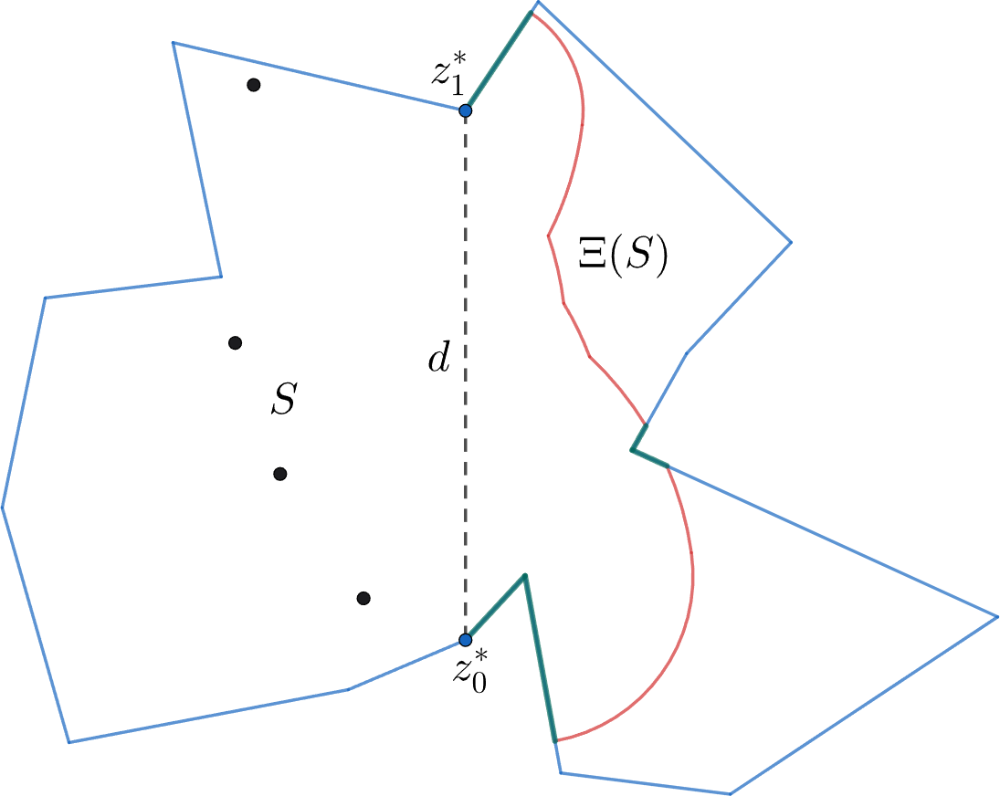
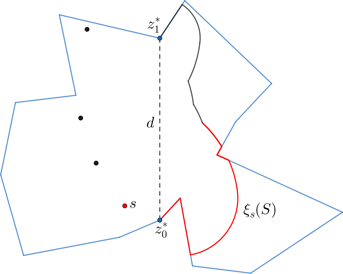
Roughly speaking, the right envelope of is the boundary of excluding . Specifically, is union of and , with and . In general, is a collection of circular arcs each belonging to for some point , while is a collection of segments on ; see Figure 3(a).
Note that may have multiple connected components. We can show that for each connected component of , consists of a single segment of and is simply connected (i.e., there are no holes), meaning that is composed of a segment of and a simple curve connecting the two endpoints of .
For any point , define as the set of points such that for any other point . In other words, if we consider the geodesic Voronoi diagram of , then consists of all points in the Voronoi region of ; see Figure 3(b). A useful property is that if , then is a single connected portion of .
Answering queries using the right envelope.
Intuitively, for any point , if and only if is “to the left of” . However, the question is how to interpret “left.”
In the Euclidean case where is the entire plane and becomes a vertical line, is a -monotone curve. Due to this property, there is a trivial way to determine whether is to the left of : First find by binary search the arc of intersecting the horizontal line through , and then determine whether is to the left of the arc [14, 30].
In our problem, however, is no longer -monotone. Intuitively, this is because is not “large enough” and changes the “shape” of . Thus, we need a new approach. At a very high level, our strategy is to develop some concepts analogous to those in the Euclidean case. Specifically, we introduce an order for any two points of ; this order corresponds to the -coordinate order in the Euclidean case. We also define a traversal order for any two points of ; in the Euclidean case, this would be the order of traversing on from bottom to top as is -monotone. In addition, we define an order for all points of based on their geodesic distances to the lower endpoint of (i.e., for any two points , define if ). A useful property is that these three orders are consistent with each other, which is crucial to the success of our approach.
A brief data structure description.
Our data structure is a complete binary tree whose leaves from left to right store the points of under the order . For each node , let be the subset of points stored in the leaves of the subtree rooted at . We wish to store an implicit representation of at . Let be the set of points such that . We consider a list of its points sorted under .
If is the root, then we store at explicitly. If we store at explicitly for all nodes , then would take super-linear space. We instead employ a standard space saving technique [18, 26], where we store a point in the highest node such that . Using this strategy, the total space of is .
For a node with left child and right child , define , i.e., among all points in , is the largest one following the order . Symmetrically, define . We can show that is a prefix of and is a suffix of . Hence, is the concatenation of and , where the notation represents the prefix of up to and including and represents the suffix of from and including . We store both and at . As is the concatenation of and , we only store in a list at and similarly store in at . This means that in a descent from the root of , we can do the following. Let be the current node in our descent and assume , which is true initially when is the root. Suppose has left child and right child . We can cut at to obtain and . As is stored in , we can concatenate and to obtain . We can do likewise to obtain . In an ascent, we can simply reverse this process to obtain from and using and . To facilitate the queries, additional information will also be maintained such as the endpoints of for each point .
5 The unweighted simple polygon case
In this section, we present our SSSP algorithm for unweighted when is a simple polygon. To solve the problem, a natural idea is to see whether the algorithms for the Euclidean case can be adapted. Two algorithms are known that can solve the Euclidean case in time [8, 9]. The algorithm in [9] relies on constructing a grid in the plane, which seems inherently not applicable to the polygon setting as explained in Section 1.1.
We therefore adapt the approach of [8]. After introducing notation, we first describe the algorithm at a high level and then discuss its implementation and time analysis.
5.1 Notation
We follow the notation already defined in Sections 1 and 2, including , , , , , , , , . For any subset and a point , let denote the nearest neighbor of in and . Note that .
We define for to be the set of vertices of whose shortest path lengths from in are equal to . Clearly, . Define .
Our goal is to compute the sets , for . In our discussion, we will focus on describing the algorithm to compute these sets. By slightly modifying the algorithm, we can also compute the predecessor information of the shortest paths.
Let denote the set of vertices of , which are also referred to as obstacle vertices. For ease of exposition, we make the following general position assumptions: (1) the shortest paths in between any two points in are unique, and (2) no point in is equidistant (in geodesic distance) to two other points in . Note that the second assumption implies that no obstacle vertex lies on a Voronoi edge of , which further means that each Voronoi edge of is one-dimensional. The second assumption also implies that the nearest neighbor of a site in any subset , i.e., , is unique.
We use to denote the dual graph of . Specifically, the vertex set of is , and two sites have an edge in if their Voronoi regions in share a Voronoi edge, i.e., . For any site , we define as the set of vertices of adjacent to ; we also refer to sites of as neighbors of in . For a subset , by slightly abusing the notation, we let .
5.2 Algorithm description
We first construct the geodesic Voronoi diagram . The algorithm then proceeds in iterations. Initially, we have . In the -th iteration for , we compute the set as follows. We assume that is available. Let , i.e., the sites in adjacent to those of in but not in . For each site , we remove from and determine whether . If so, we add to . In addition, we update , i.e., add the sites of that are not in to for the current . We repeat this until becomes empty. The -th iteration finishes once become empty. If , then the algorithm stops; otherwise, we proceed with the next iteration. See Algorithm 1 for the pseudocode.
Correctness.
It is not obvious why the algorithm is correct. See the full paper for the proof.
5.3 Algorithm implementation and time analysis
First of all, computing can be done in time [24] (see also [2, 27, 25] for other algorithms). Note that the combinatorial size of is [2]. Therefore, can be obtained from in additional linear time. In addition, since has vertices and is a planar graph, has edges.
Throughout the whole algorithm, each edge of is considered at most four times (twice for each vertex) in the construction of the neighborhood sets. Specifically, the edge for will be considered by Line 9 in the -th iteration and by Line 4 in the -th iteration. There are edges in , so there are at most insertions (and thus pop operations) to . Hence, the while loop on Line 5 has at most iterations throughout the whole algorithm. It remains to determine the time complexity for the operation of checking whether on Line 7.
Notice that if and only if has a point with . Hence, the problem can be solved by a geodesic unit-disk range emptiness (GUDRE) query. Using Theorem 1, we construct a GUDRE data structure for in time at the beginning of each -th iteration of Algorithm 1. Using a GUDRE query, whether can be determined in time by Theorem 1. Note that no deletions on are needed. Since , the overall time for constructing the GUDRE data structure for in all iterations of the algorithm is .
We conclude that the total time of the algorithm is , which is .
Theorem 6.
Given a simple polygon of vertices, a set of points in , and a source point , we can compute shortest paths from to all points of in the geodesic unit-disk graph of in time.
6 The unweighted polygonal domain case
When is a polygonal domain with holes, the framework of Algorithm 1 continues to apply. The main difficulty is algorithmic. Unlike the simple polygon setting, we do not have an efficient analogue of Theorem 1 for polygonal domains (even without deletions) that would allow us to evaluate the condition on Line 7.
As before, the algorithm proceeds in iterations, with the th iteration responsible for computing . Our key idea is to distinguish between iterations based on the size of . If , we classify the iteration as heavy; otherwise, it is light. We design separate procedures for these two types, referred to as the heavy-iteration procedure and the light-iteration procedure, respectively. At the start of iteration , the value of is not known in advance. Our strategy is therefore to always begin with the light-iteration procedure. If, during its execution, more than sites are discovered for , we immediately abort the light-iteration procedure and switch to the heavy-iteration procedure.
A useful observation is that there can be at most heavy iterations, since the sets are disjoint, their union is , and each heavy iteration has at least sites.
We only give a very brief sketch below. See the full paper for the details. We follow the notation and the discussion in Section 5.1. While the heavy-iteration procedure is relatively easy, the light procedure is quite interesting.
Heavy-iteration procedure.
We compute the geodesic Voronoi diagram of in in time. With the diagram and a point location data structure, for each site , we can compute and its geodesic distance from in time [19]; note that their geodesic distance is . If , we add to . This computes in time, which is . Since the number of heavy iterations in the entire algorithm is , the total time of all heavy procedures in the algorithm is .
Light-iteration procedure.
The procedure runs in rounds, and each round computes at least one new point for . If a round does not compute any new point for , then we can assert that all sites of have been computed. If after a round becomes larger than or equal to , then we terminate the procedure and switch to the heavy-iteration procedure.
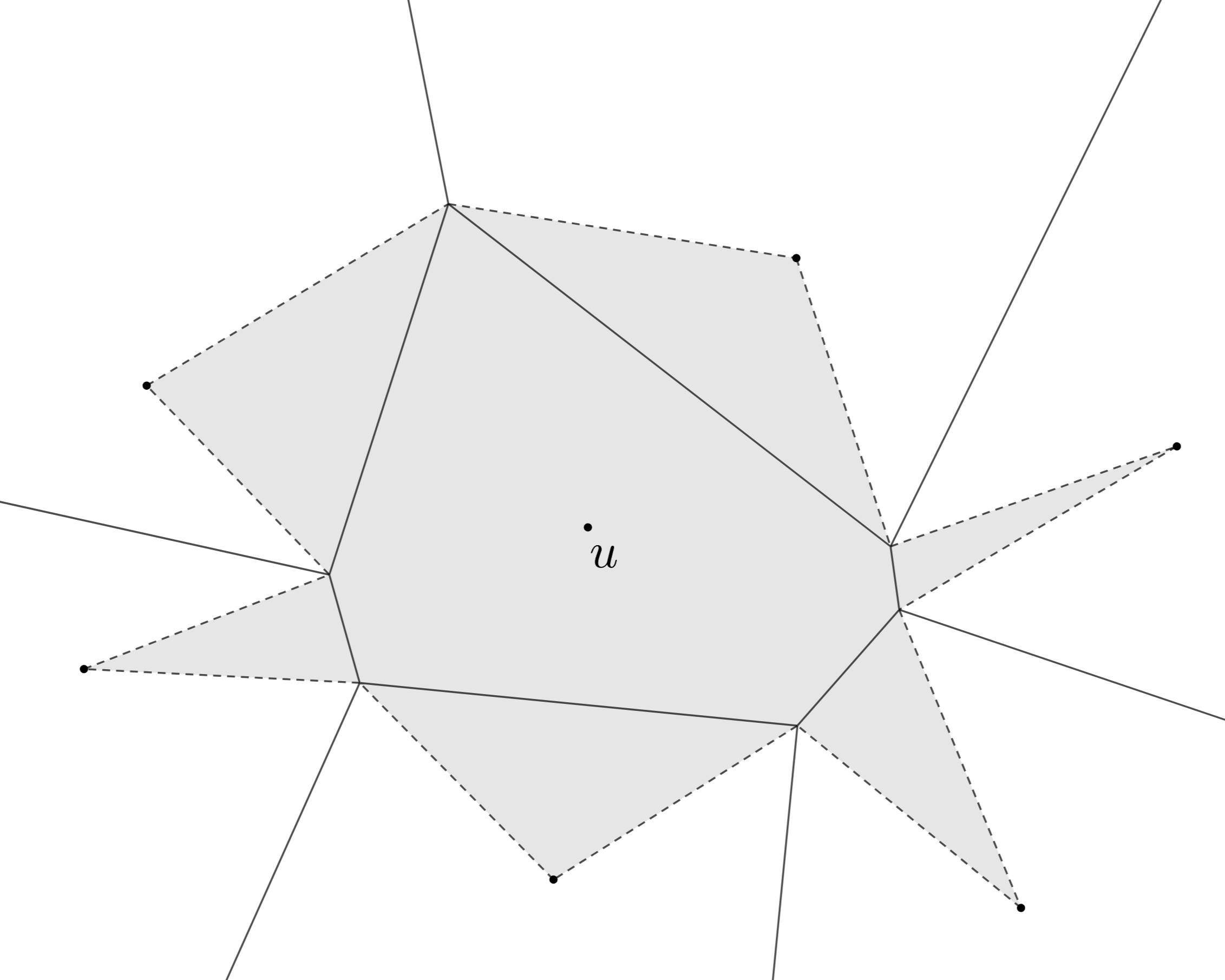
In each round, we search in the neighborhoods of the sites of and the current . We find that we do not need in the entire to conduct this search, and only a “small portion” of it suffices. More specifically, suppose there is a shortest path from a site of to and enters through for a neighbor . Consider the Voronoi edge of between and . This edge may be comprised of multiple connected components where each component is a sequence of hyperbolic arcs. For each component , let be the subregion of bounded by , , and , where and are the two endpoints of (note that and must be in ). We observe that for any point in , there exists a shortest path that is inside . Therefore, if we want to include the shortest path through , the only portion of that we need to include when constructing the Voronoi diagram for is union of for all components . See Figure 4. Motivated by this, for each site , we define to be the union of and all for all and all connected components ; see Figure 5. By including in our “work region” for computing the Voronoi diagram for , we ensure that for all , if crosses , then this path will be included in our work region. This leads to a total of time for all light procedures.
References
- [1] Pankaj K. Agarwal, Lars Arge, and Frank Staals. Improved Dynamic Geodesic Nearest Neighbor Searching in a Simple Polygon. In Proceedings of the 34th International Symposium on Computational Geometry (SoCG), pages 4:1–4:14, 2018. doi:10.4230/LIPIcs.SoCG.2018.4.
- [2] Boris Aronov. On the geodesic Voronoi diagram of point sites in a simple polygon. Algorithmica, 4:109–140, 1989. doi:10.1007/BF01553882.
- [3] Jon L. Bentley. Decomposable searching problems. Information Processing Letters, 8:244–251, 1979. doi:10.1016/0020-0190(79)90117-0.
- [4] Mark de Berg, Sándor Kisfaludi-Bak, Morteza Monemizadeh, and Leonidas Theocharous. Clique-based separators for geometric intersection graphs. Algorithmica, 85:1652–1678, 2022. doi:10.1007/s00453-022-01041-8.
- [5] Magdalene G. Borgelt, Marc van Kreveld, and Jun Luo. Geodesic disks and clustering in a simple polygon. In Proceedings of the 18th International Conference on Algorithms and Computation (ISAAC), pages 656–667, 2007. doi:10.5555/1781574.1781647.
- [6] Prosenjit Bose, Paz Carmi, and Thomas C. Shermer. Piercing pairwise intersecting geodesic disks. Computational Geometry: Theory and Applications, 98(101774), 2021. doi:10.1016/j.comgeo.2021.101774.
- [7] Bruce W. Brewer and Haitao Wang. An improved algorithm for shortest paths in weighted unit-disk graphs. In Proceedings of the 36th Canadian Conference on Computational Geometry (CCCG), pages 57–64, 2024. arXiv:2407.03176.
- [8] Sergio Cabello and Miha Jejčič. Shortest paths in intersection graphs of unit disks. Computational Geometry: Theory and Applications, 48:360–367, 2015. doi:10.1016/j.comgeo.2014.12.003.
- [9] Timothy M. Chan and Dimitrios Skrepetos. All-pairs shortest paths in unit-disk graphs in slightly subquadratic time. In Proceedings of the 27th International Symposium on Algorithms and Computation (ISAAC), pages 24:1–24:13, 2016. doi:10.4230/LIPIcs.ISAAC.2016.24.
- [10] Bernard Chazelle. Cutting hyperplanes for divide-and-conquer. Discrete and Computational Geometry, 9(2):145–158, 1993. doi:10.1007/BF02189314.
- [11] Bernard Chazelle and Leonidas J. Guibas. Visibility and intersection problems in plane geometry. Discrete and Computational Geometry, 4:551–589, 1989. doi:10.1007/BF02187747.
- [12] Brent N. Clark, Charles J. Colbourn, and David S. Johnson. Unit disk graphs. Discrete Mathematics, 86:165–177, 1990. doi:10.1016/0012-365X(90)90358-O.
- [13] Herbert Edelsbrunner, Leonidas J. Guibas, and Jorge Stolfi. Optimal point location in a monotone subdivision. SIAM Journal on Computing, 15(2):317–340, 1986. doi:10.1137/0215023.
- [14] Alon Efrat, A. Itai, and Matthew J. Katz. Geometry helps in bottleneck matching and related problems. Algorithmica, 31(1):1–28, 2001. doi:10.1007/s00453-001-0016-8.
- [15] Leonidas J. Guibas and John Hershberger. Optimal shortest path queries in a simple polygon. Journal of Computer and System Sciences, 39:126–152, 1989. doi:10.1016/0022-0000(89)90041-X.
- [16] Leonidas J. Guibas, John Hershberger, Daniel Leven, Micha Sharir, and Robert E. Tarjan. Linear-time algorithms for visibility and shortest path problems inside triangulated simple polygons. Algorithmica, 2:209–233, 1987. doi:10.1007/BF01840360.
- [17] John Hershberger. A new data structure for shortest path queries in a simple polygon. Information Processing Letters, 38(5):231–235, 1991. doi:10.1016/0020-0190(91)90064-O.
- [18] John Hershberger and Subhash Suri. Applications of a semi-dynamic convex hull algorithm. BIT, 32:249–267, 1992. doi:10.1007/BF01994880.
- [19] John Hershberger and Subhash Suri. An optimal algorithm for Euclidean shortest paths in the plane. SIAM Journal on Computing, 28(6):2215–2256, 1999. doi:10.1137/S0097539795289604.
- [20] Haim Kaplan, Wolfgang Mulzer, Liam Roditty, Paul Seiferth, and Micha Sharir. Dynamic planar Voronoi diagrams for general distance functions and their algorithmic applications. Discrete and Computational Geometry, 64:838–904, 2020. doi:10.1007/s00454-020-00243-7.
- [21] David G. Kirkpatrick. Optimal search in planar subdivisions. SIAM Journal on Computing, 12:28–35, 1983. doi:10.1137/0212002.
- [22] D.T. Lee and Franco P. Preparata. Euclidean shortest paths in the presence of rectilinear barriers. Networks, 14(3):393–410, 1984. doi:10.1002/net.3230140304.
- [23] Chih-Hung Liu. Nearly optimal planar nearest neighbors queries under general distance functions. SIAM Journal on Computing, 51:723–765, 2022. doi:10.1137/20M1388371.
- [24] Eunjin Oh. Optimal algorithm for geodesic nearest-point Voronoi diagrams in simple polygons. In Proceedings of the 20th Annual ACM-SIAM Symposium on Discrete Algorithms (SODA), pages 391–409, 2019. doi:10.1137/1.9781611975482.25.
- [25] Eunjin Oh and Hee-Kap Ahn. Voronoi diagrams for a moderate-sized point-set in a simple polygon. Discrete and Computational Geometry, 63:418–454, 2020. doi:10.1007/s00454-019-00063-4.
- [26] Mark H. Overmars and Jan van Leeuwen. Maintenance of configurations in the plane. Journal of Computer and System Sciences, 23(2):166–204, 1981. doi:10.1016/0022-0000(81)90012-X.
- [27] Evanthia Papadopoulou and D.T. Lee. A new approach for the geodesic Voronoi diagram of points in a simple polygon and other restricted polygonal domains. Algorithmica, 20:319–352, 1998. doi:10.1007/PL00009199.
- [28] Liam Roditty and Michael Segal. On bounded leg shortest paths problems. Algorithmica, 59:583–600, 2011. doi:10.1007/s00453-009-9322-3.
- [29] Haitao Wang and Jie Xue. Near-optimal algorithms for shortest paths in weighted unit-disk graphs. Discrete and Computational Geometry, 64:1141–1166, 2020. doi:10.1007/s00454-020-00219-7.
- [30] Haitao Wang and Yiming Zhao. Computing the minimum bottleneck moving spanning tree. Algorithmica, 22:6:1–6:22, 2026. doi:10.1007/s00453-025-01358-0.