The Squishy Grid Problem

Abstract
In this paper we consider the problem of approximating Euclidean distances by the infinite integer grid graph. Although the topology of the graph is fixed, we have control over the edge-weight assignment , and hope to have grid distances be asymptotically isometric to Euclidean distances, that is:
| For all grid points , . |
We give three methods for solving this problem, each attractive in its own way.
-
Our first construction is based on an embedding of the recursive, non-periodic pinwheel tiling of Radin and Conway [15, 16, 9] into the integer grid. Distances in the pinwheel graph are asymptotically isometric to Euclidean distances, but no explicit bound on the rate of convergence was known. We prove that the multiplicative distortion of the pinwheel graph is , where is the Euclidean distance and . The pinwheel tiling approach is conceptually simple, but can be improved quantitatively.
-
Our second construction is based on a hierarchical arrangement of highways. It is simple, achieving stretch , which converges doubly exponentially faster than the pinwheel tiling approach.
-
The first two methods are deterministic, with rigorous guarantees. An even simpler approach is to sample the edge weights independently and randomly from a common distribution . Whether there exists a distribution that makes grid distances Euclidean, asymptotically and in expectation, is major open problem in the theory of first passage percolation. Previous experiments show that when is a Fisher distribution (which is continuous), grid distances are within of Euclidean distances. We demonstrate experimentally that this level of accuracy can be achieved by a simple 2-point distribution that assigns weights or with probability % and %, respectively.
Keywords and phrases:
grid graph, Euclidean distance, metric embedding, first passage percolationCopyright and License:
![[Uncaptioned image]](x1.png) © Zixi Cai, Kuowen Chen, Shengquan Du, Arnold Filtser, Seth Pettie, and Daniel Skora; licensed under Creative Commons License CC-BY 4.0
© Zixi Cai, Kuowen Chen, Shengquan Du, Arnold Filtser, Seth Pettie, and Daniel Skora; licensed under Creative Commons License CC-BY 4.0
2012 ACM Subject Classification:
Theory of computation Randomness, geometry and discrete structuresFunding:
Supported by NSF Grants CCF-2221980 and CCF-2446604 and Israel Science Foundation Grant No. 1042/22.Editors:
Hee-Kap Ahn, Michael Hoffmann, and Amir NayyeriSeries and Publisher:
 Leibniz International Proceedings in Informatics, Schloss Dagstuhl – Leibniz-Zentrum für Informatik
1 Introduction
In this paper we consider a natural geometric problem tangentially related to metric embeddings, spanners, and, in its randomized form, percolation theory. Suppose we wish to approximate Euclidean distances between points on the plane, but with a simple discrete structure: the integer grid graph . If we consider all edges of to have unit length, then can be regarded as a -spanner since for any ,
Now define to be endowed with a non-negative edge-weight assignment , and let be the distance function with respect to . We consider the natural question: does there exist a that is an asymptotic 1-spanner of the Euclidean plane?
Question 1 (The Squishy Grid Problem).
Does there exist a weight function such that for all is asymptotically Euclidean? That is,
If so, we may distinguish various types of convergence:
- Polynomial.
-
.
- Subpolynomial.
-
.
- Constant.
-
.
Before discussing our approach to answering Question 1 we review the history of Question 1 and its connections to percolation theory.
1.1 History of the Problem and Related Results
G. Tardos (personal communication) made us aware of a 1990 book chapter of Pach, Pollack, and Spencer [14] who attributed some version of Question 1 to Paul Erdős. Pach et al. [14] proved that for any fixed there exists a graph on the vertex set such that for all ,
Unfortunately, is not planar and obviously depends on , so it does not lead to a resolution of Question 1. Burago and Ivanov [6] exhibited a regular, weighted graph on the vertex set for which
for some absolute constant . However, is also not planar.
Borradaile and Eppstein [4] considered a more general problem: given a point set , compute a weighted planar graph with Steiner points such that -approximates the Euclidean distance . They proved that suffices, where is the sharpest angle in the Delaunay triangulation of . A result of Chang, Krauthgamer, and Tan [8] implies an upper bound of , which is slightly superlinear but independent of .
The problem was first posed to us by G. Bodwin, not as a deterministic design problem (Question 1) but as a randomized one. Whenever is a distribution over , let be the distribution of weighted graphs such that for each , is sampled independently from the distribution. Is it possible to find a distribution such that distances in are Euclidean in expectation? In more detail:
Question 2 (Randomized Squishy Grid Problem).
Does there exist a distribution over such that if is a randomly weighted graph, for all ,
The randomized process implicit in Question 2 is actually not new, but dates back to at least a 1965 paper of Hammersley and Welsh [11], who called it first passage percolation. They imagined an orchard in which trees were planted on the integer lattice. One tree is initially infected, and the time taken for an infected tree to infect a cardinal neighbor is governed by a distribution on . One can then ask: how far does the infection spread by time ? and what does the set of infected trees look like?
Many basic questions in first passage percolation theory remain open, and we can quickly summarize the known facts related to Question 2. Let be the origin and be the unit vector with angle degrees. We interpret to mean the integer point in nearest to . The time constant is such that almost surely, which exists if, whenever are independently sampled, [12]. It follows that , with the latter inequality holding with equality only if is constant almost surely [11]. Similarly, the time constants for other angles exist, and collectively define the limiting shape of the balls under distribution . Let be the ball of radius around the origin. The Cox-Durrett shape theorem [10] shows that with probability 1, as , tends to a fixed limit shape . When , is bounded, convex, and has the same symmetries as , and when , is itself. See [2] for an extensive survey of first passage percolation theory.
In the context of answering Question 2 we can rescale any non-trivial distribution so that its time constant , i.e., distances from the origin to points on the - and -axes are asymptotically isometric. In light of the Cox-Durrett theorem, Question 2 asks whether there exists a for which is the unit ball .
Unfortunately, there are no results characterizing for any non-trivial distribution . It is not even known whether there exists such that
| (1) |
i.e., coincides with the unit -ball on the eight (inter)cardinal directions. On the other hand, we have solid experimental evidence that can get within 1% of the unit -ball, for certain distributions . An experimental study of Alm and Deijfen [1] looked at various continuous distributions . When is the uniform distribution, the limit shape approximates the -ball to with 4%, whereas when is exponential the limit shape is about 1.5% away from the -ball. The best empirical approximation to the -ball came from a Fisher distribution, with error less than 1%.
1.2 Results and Findings
We provide two approaches to answering Question 1 and present experimental evidence that Question 2 can be answered in the affirmative, using simple discrete distributions.
Our first construction is based on Radin and Conway’s pinwheel tiling [15, 16, 9], a conceptually simple tiling that emerges from the observation that a right triangle with proportions can be partitioned into five right triangles with the same proportions. It is known [16] that when regarded as a plane graph with edges weighted according to Euclidean distance, distances in the pinwheel tiling are Euclidean in the limit, that is,
However the rate of convergence is unknown. We embed the pinwheel tiling into the grid graph, and prove a bound on its convergence, namely that for a constant ,
A natural problem is to optimize the convergence rate of the construction. We give a new, simple construction of a weight function of the grid that is asymptotically Euclidean, with a polynomial convergence rate, namely: .
The construction is based on laying out “highways” in the plane, which are paths cleaving closely to a line with a certain slope , whose edge weights are equal and chosen to approximate Euclidean distances along the highway. For example, when , the weights are . In order to get a -distance approximation, it is necessary that the set of slopes of all highways be dense in . Thus, there are infinitely many slopes, and infinitely many parallel highways of each slope, whose intersection pattern is quite complicated. The tricky part in the design stage is to decide what to do with intersecting highways. We give a simple method that eliminates intersections while guaranteeing polynomial convergence.
Alm and Deijfen’s [1] experimental study of first passage percolation selected from various continuous distributions such as uniform, exponential, Gamma, and Fisher distributions. For several of these distributions the limit shape approximated the -ball within a few percent, with a Fisher distribution being the best. Our experiments show that very simple distributions with support size 2 or 3 can replicate the accuracy of the continuous distributions [1]. For example, the improbable distribution :
empirically approximates the Euclidean metric to within about , and a certain 3-point distribution approximates it to within . A very natural question is whether other metrics can be approximated, in expectation, by various distributions. We illustrate that the uniform distribution and some Gamma distributions approximate metrics with . None of our experiments support the possibility that metrics with can be approximated.
1.3 Organization
We present the construction based on pinwheel tilings in Section 2, as well as new bounds on the convergence of the stretch of the pinwheel graph. The highway construction is presented in Section 3, having polynomial convergence. We present the experimental findings in Section 4 and conclude with a discussion of several open problems related to Questions 1 and 2 in Section 5. Sections 2, 3, and 4 are written to be independent.
2 A Deterministic Construction Based on Pinwheel Tilings
The “pinwheel” tiling of Radin [15] is an example of a non-periodic tiling using a single tile type (and its reflection). Let be a series of tilings of ever larger triangular swatches of the plane, and let be the tesselation of the plane achieved in the limit. consists of a single right triangle with side lengths . In general is formed from by taking four additional copies of , suitably reflected, rotated, and translated, so that they form a larger triangle with the same proportions. Figure 1 illustrates the construction of from and .
2.1 Pinwheel Tilings
By construction is a tiling of the plane using atomic triangles with side lengths . Due to the recursive nature of the construction, we can also regard as a tiling using triangles, for any integer . Observe from Figure 1 that the boundary of is obtained from the boundary by scaling by , translation, and rotation by . We will henceforth define . As is irrational, the orientation of tiles in is uniformly distributed in . Radin and Sadun [16] used this fact to prove an isoperimetric property of pinwheel tilings, namely that there are finite subsets of tiles from whose area/perimeter2 is arbitrarily close to that of the circle. Suppose we regard as a plane graph , whose vertices and edges are the union of the vertices and edges of all atomic triangles. Radin and Sadun [16] proved that for , . Although the multiplicative stretch is 1 in the limit, their proof implies no particular rate of convergence. We prove the following.
| (A) | (B) |
Theorem 1.
Let be the plane graph of the pinwheel tiling , whose edges are weighted according to the Euclidean distance between their endpoints. Then for any ,
2.2 Distribution of Tile Orientations
If is a triangle in the recursive tiling with dimensions , we call a level- triangle. As a first step toward proving Theorem 1, we analyze the orientations of the triangles contained within a single large triangle. Given a triangle of level , let denote the set of angles attained by the hypotenuses of all level- triangles contained within . We observe that the elements of this set are characterized by an arithmetic recurrence.
Observation 2.
Suppose a triangle of level has its hypotenuse at angle . For , .
Proof.
We proceed by induction on , with the base case being trivial. Consult Figure 2, where two triangles and of level- are depicted. Observe that the hypotenuse of (resp. ) is rotated by an angle of (resp. ) relative to that of the exterior triangle. By the inductive hypothesis,
and the union of these sets is exactly .
Consider some , and denote by the fractional part of . It is well known due to Weyl’s criterion that if is irrational, the set becomes uniformly distributed in as [5]. Moreover, the rate of convergence is controlled by the irrationality exponent which measures the asymptotic quality of rational approximations to . For a real number , is defined to be the supremum of the set of real numbers such that has infinitely many solutions for integers with . A finite irrationality exponent implies that a number does not have a sequence of rational approximations that are “too good.” For sets , we say is an -cover of if for every there exists satisfying . When is finite, is an -cover of for [13]. The following corollary follows by applying this fact to Observation 2.
Corollary 3.
Given a triangle of level-, is a -cover of for .
Before bounding the irrationality exponent , we quickly review some terminology related to the algebraic numbers . For , its minimal polynomial is the unique polynomial of lowest degree with relatively prime coefficients such that . We say the degree of is the degree of , while the height of is the absolute value over coefficients of .
Both and can be expressed in the form where and . Since , . Similarly, can be written as . A great deal of work in the mid-20th century yielded various lower bounds on linear forms in logarithms of algebraic numbers. A history of the problem up to 1976 can be found in [3]. For our purposes, we choose a simple bound due to Baker.
Theorem 4 (Baker [3]).
Suppose for we have algebraic numbers . If the logarithms are linearly independent over the rational numbers, then
where is the maximum of the heights of the and is a function of , the numbers , and the degrees of the numbers .
Consider arithmetic expressions of the form where are fixed and . Now and have degree , so the exponent becomes a constant, and . Applying Baker’s theorem (Theorem 4) and dividing both sides by yields . By choosing and , the ratio is exactly . Recall that this number is irrational, satisfying the criteria that and are linearly independent over the rationals. Since , clearly we can replace by to obtain . Comparing this with the definition of the irrationality exponent, this is sufficient to see that is at most and therefore finite. Henceforth let . It is worth noting that the constant given by Theorem 4 is effectively computable, though the order of magnitude is impractical.111One estimate, also due to Baker [3], states that suffices when the are rational, where is the height of and is the degree of the field extension . For our purposes, , , , and , giving . Baker remarks it is possible to argue is much lower in reality, but the required analysis is quite technical and beyond the scope of this paper.
2.3 Convergence of Stretch
We define to be the maximum stretch guaranteed by , over all pairs of vertices at Euclidean distance at least .
Lemma 5.
Fix any distance and let . There exists a function such that if , then .
Proof.
Consider any two vertices with when we regard them as points in the plane. Begin by choosing a parameter and identifying a triangle satisfying the following properties: intersects , the projection of onto lies entirely within the middle third of , and the hypotenuse of has length exactly . Now choose a parameter and let be large enough such that is a -cover of . Finally, select a triangle within , and exactly levels below , whose hypotenuse creates an angle less than with .
We now construct a path as follows. Let and be the endpoints of the hypotenuse of closer to and respectively. Let , , and . and must each be at least , so by the definition of the stretch function , approximates and to within stretch.
Let , , and be the projections of , , and onto . We claim that . Since lies within , its projection onto is a distance at most from and at least from . Therefore, is bounded by . By definition of , . The same is true for . On the other hand, is trivially bounded by since and are joined directly by an edge in . Combining the bounds on each component, we write
We normalize by to obtain the stretch, and because this inequality holds for arbitrary satisfying , it holds for the supremum as well.
| Letting , this is upper bounded by | ||||
| At this point we fix , so . | ||||
| Finally, we pick . | ||||
By Corollary 3, we choose . The only remaining detail is to address that the triangles and used in this argument do indeed exist. The length of the hypotenuse of was taken to be , and then we chose to be levels beneath that of . Therefore, we have implicitly assumed , consistent with the assumption in the statement of the lemma.
2.4 Pinwheel Tilings on the Grid
Theorem 6.
There exists a weight function such that has stretch 1, asymptotically. In particular, for any ,
The proof of this theorem can be found in the full version [7].
3 A Deterministic Construction with Faster Convergence
In this section, we give a deterministic construction based on highways with faster convergence. Specifically, we establish the following result as Theorem 7:
Theorem 7.
There exists an assignment such that for any ,
We prove Theorem 7 in two steps. First, we show that the same statement holds for the finite square grid (Theorem 8), then we give a black-box reduction from the infinite case to the finite case.
Theorem 8.
There exists a weight assignment to edges of the finite grid on such that for any ,
The proof of Theorem 8 follows from the constructions presented in Section 3.1 and Section 3.2.
3.1 Highways
Given a line in we define the to be a grid-path that tracks ; see Figure 3.
Specifically, let be a grid-point, and consider the square . If intersects this square, then we include in . Whenever are adjacent grid points, contains the edge . If we let assign every edge in the weight , which is the asymptotic ratio between the Euclidean distance of points on and the number of edges taken along the grid path . Otherwise we write as with and use weight . All off-highway edges have weight .
This weight assignment guarantees a discrepancy of at most 1 between Euclidean distances and grid distances along . The proof of Lemma 9 appears in [7].
Lemma 9.
Let denote the highway that approximates a line of the form . Then for any two points , .
The highway transformation can also be applied to a line segment . We use the same notation .
3.2 The Hierarchical Highway Construction
We are trying to find a weight assignment for the finite grid in order to prove Theorem 8. The construction is parameterized by , where , and is minimum such that .
The construction is based on a hierarchical system of lines in which will eventually be embedded as highways in the grid. The lines at level have angles selected from , where . Fixing and one such angle , there are many lines with angle , spaced at distance . For , define
Define to be the set of all lines at level .
We cannot choose a weight function that agrees with for every line due to intersections. Our solution is to avoid this issue by removing all line intersections, which introduces distortions in distances that must be bounded.
Below we define a procedure to remove parts of , leaving a set of line segments . Define to be the set of all line segments at level . If is an object or collection of objects, define
to be all points within distance of . Specifically, is a strip if is a line, and a hippodrome if is a segment.
Once are constructed, we construct as follows. For each initialize and proceed to remove parts of in Steps 1 and 2.
- Step 1.
-
Set , i.e., we remove every part of within distance of any other line at level .
- Step 2.
-
For each segment such that , let . If , set . Otherwise, let be such that and , and set . See Figure 4. Define , and include all line segments of in .
| (A) |
| (B) |
The weight assignment is now constructed as follows. For each line segment , let agree with at all edges in the corresponding highway segment . All edges not appearing in any line segment have weight 2.
Lemma 10.
Fix any , , where and . For any points , .
Proof.
Steps 1 and 2 ensure that all remaining points on lie outside
and that any two consecutive segments on are separated by distance at least . This implies that the Euclidean distance between any and is at least .
Lemma 11 shows that distances under are approximately Euclidean, up to a multiplicative stretch of and additive stretch , for every index .
Lemma 11.
For any and .
Proof.
Observe that the highways corresponding to all segments in are vertex-disjoint. Thus, every grid path from to can be written as , where each for some and each is disjoint from all highway segments, and therefore consists of only weight-2 edges. (One or both of may be empty.) By Lemma 9, is at least the Euclidean distance between its endpoints minus one, and is at least the Euclidean distance multiplied by 2, which implies that is at least the Euclidean distance plus 1 for , so is at least .
Turning to the upper bound, We bound the distance by explicitly constructing a path that stays within the vicinity of a single line . Since level- lines occur at angular intervals of and parallel lines are spaced apart, we can always find an satisfying the following properties. First, the difference in angle between and is at most . Second, the distance from to is at most . Let and be the closest grid points on from and respectively. It follows that
| (2) |
It remains to bound . A trivial upper bound is , so if we are done. Henceforth we shall assume that . We would prefer to follow the - path along , but sections of this highway have effectively been removed by Steps 1 and 2 of the construction. We bound the stretch induced by the gaps in the highway introduced in Steps 1 and 2 separately.
Step 1 Stretch.
Fix a direction different from ’s direction . Whenever intersects a line with angle , Step 1 causes to lose edges. There are angles, and parallel lines with angle are spaced apart, so the total number of edges removed from the - path in in Step 1 is
| (3) |
The additive stretch induced by walking across the gaps induced by Step 1 is also as all these edges have weight 2.
Step 2 Stretch.
Whenever part of is removed by Step 2 we do not walk precisely in the direction of but take a detour to a lower level highway. Suppose that in Step 2, a segment causes an interval of to be removed. Define to be the points on closest to , respectively. When our path reaches , we walk from to , then to along , then to . See Figure 5. By construction . Since and by Lemma 9 , the additive stretch due to the conflict with is at most
The last task is to bound the number of such segments interfering with the - path. Observe that is a segment of a line at level or lower. Thus, by Lemma 10 any two such segments are at distance at least , and the total additive stretch caused by Step 2 detours is
| (4) |
| (A) |
| (B) |
Combining Equations 2, 3, and 4, we conclude that
Proof of Theorem 8.
4 Experimental Findings in the Squishy Grid
If Question 2 seems too daunting, a natural idea is to simplify the problem by considering only monotone paths, that is, paths that use the fewest number of edges.
Question 3.
Define to be the length of the shortest - path that uses edges. Is there a distribution over such that if is a randomly weighted graph, for all , ?
At first glance this problem may seem easier, or more plausible, than Question 2. Whereas it is an open problem finding a distribution satisfying Equation 1 (the time constant in the and directions are 1), this is nearly trivial when we consider . Refer to [7] for proof.
Lemma 12.
There exists a distribution on such that
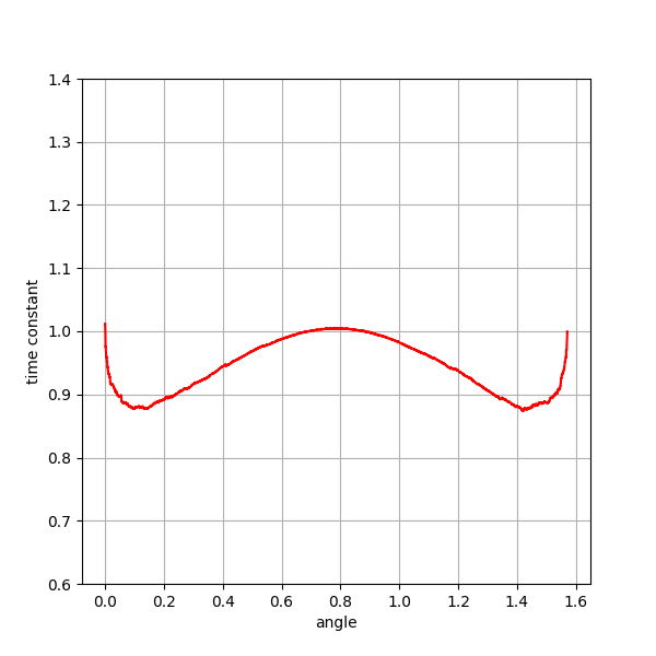
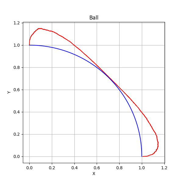
Let and be the limiting shape of in as . Thus, coincides with the -ball in the eight intercardinal directions N, E, S, W, NE, SE, SW, NW. If were convex, then it would have to be quite close to the -ball. Unfortunately, our experiments show that is not convex, which casts serious doubt on Question 3 having an affirmative answer. See Figure 6.
 |
 |
| (A) | (B) |
In retrospect, Question 3 is less likely than Question 2 to be answered in the affirmative since , , is much more sensitive to small deviations in than Considering the cases when , and , is the minimum of , and different paths, respectively. This sharp jump from constant to exponential in the vicinity does not exist in Question 2. Assuming the variance of is sufficiently large, is the minimum of an exponential number of plausible shortest paths.
4.1 Discrete Distributions for First Passage Percolation
When dealing with discrete distributions the most natural measure of complexity is support size. Therefore, we study Question 2 experimentally by considering the space of 2- and 3-point distributions. For a fixed integer , the -point distribution , is such that . It is determined by parameters, as .
4.1.1 Experimental Methodology
To identify locally optimal distributions among -point discrete distributions of the form , we employ a two-layer iterative strategy:
-
We first perturb the probability vector .
-
For fixed probabilities , we generate random initial values and then alternate between the following two update steps:
- Perturbation Step.
-
We perturb each value and compute the estimated directional stretch for both and . Let be the empirical ratio , obtained from this round of simulation. Here 30,000.
- Normalization Step.
-
We normalize the values by setting . This scaling ensures that the average stretch along the cardinal and intercardinal directions remains close to 1, thereby facilitating comparisons between distributions.
4.1.2 2-Point Distributions
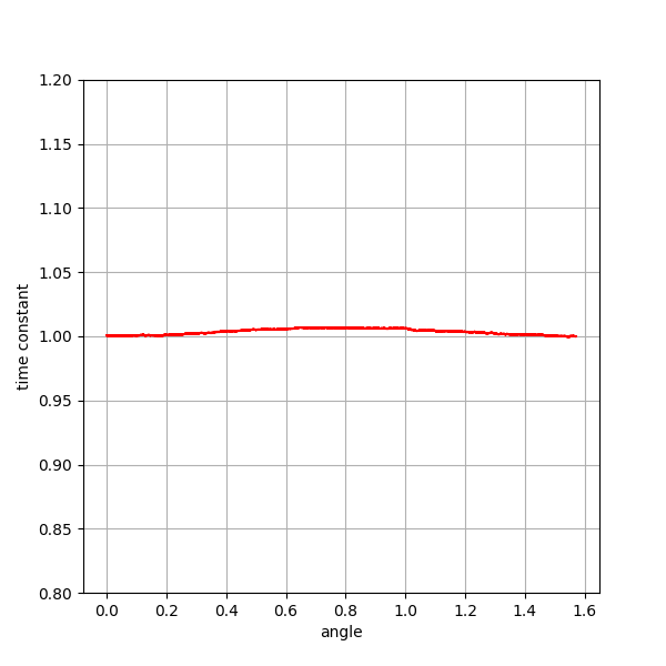
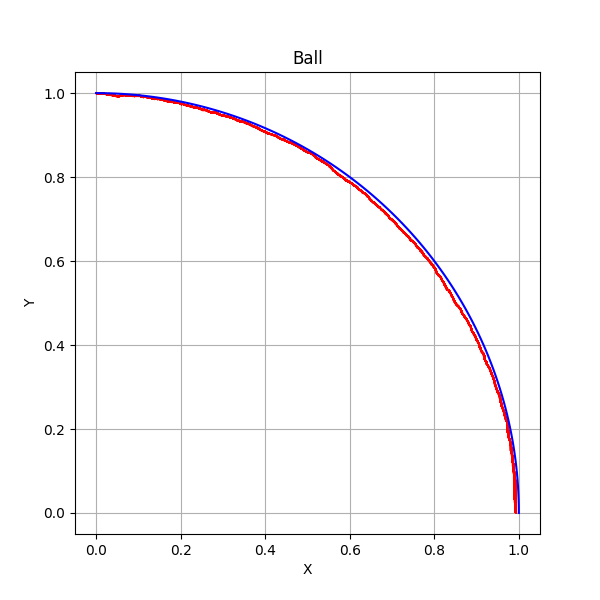
The best -point distribution identified with this method is , given below. Roughly speaking, every edge weight is either or , % and % of the time, respectively.
We find that empirically approximates Euclidean distances up to stretch , i.e., up to error. Figure 7(A) plots the observed stretch as a function of the angle . Figure 7(B) shows the set of all grid points whose empirical graph distance from the origin first exceeds . The resulting boundary is visually close to a Euclidean circle, suggesting that induces an approximately isotropic metric in expectation.
 |
 |
| (A) | (B) |
Note that , meaning that is likely to be realized by a highly non-monotone path, consistent with the observations in Figure 6.
4.1.3 3-Point Distributions
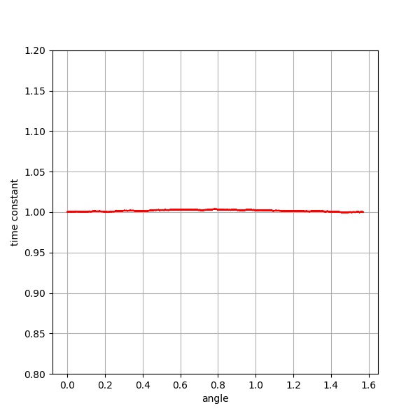
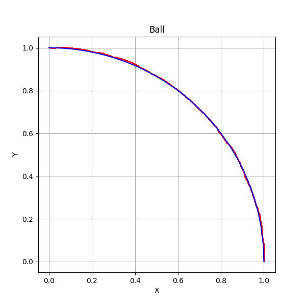
does not leave much room for improvement, but we are able to eke out a slightly better empirical stretch of 1.00622 with a 3-point distribution .
See Figure 8 for visual representations of the empirical stretch of .
 |
 |
| (A) | (B) |
5 Conclusion
In this paper we asked how well the integer grid graph can approximate Euclidean distances, if weighted appropriately. We gave two deterministic weighting schemes that answer Question 1, the best one achieving a polynomial additive stretch, that is, for . Improving the additive stretch to something subpolynomial seems to require a new approach to the problem. Our “highway” method seems incapable of achieving subpolynomial additive error, and even if Question 2 is answered affirmatively (choosing weights i.i.d. from some distribution ), the tail bounds here only give polynomial additive error [2].
We conjecture that no weighting achieves subpolynomial additive error.
Conjecture 13.
The additive error of is a function of .
- Weak Conjecture.
-
There is no with constant additive error , independent of .
- Strong Conjecture.
-
There is no with subpolynomial additive error .
In the randomized setting, Question 2 is equivalent to an old problem in first passage percolation [2, 11] that is unsolved, but has some empirical evidence in its favor. Alm and Deijfen [1] showed that when is a certain Fisher distribution, that approximates Euclidean distances to less than error. In this paper, we demonstrated that a simple 2-point distribution achieves error, and that a 3-point distribution achieves error. It is an interesting open problem to prove that in , the expected error of is less than 1%.
References
- [1] Sven Erick Alm and Maria Deijfen. First passage percolation on : A simulation study. J. Stat. Phys., 161:657–678, 2015. doi:10.1007/s10955-015-1356-0.
- [2] Antonio Auffinger, Michael Damron, and Jack Hanson. 50 Years of First-Passage Percolation. University Lecture Series. American Mathematical Society, 2017.
- [3] Alan M. Baker. The theory of linear forms in logarithms. In Transcendence theory: advances and applications (A. Baker, D. W. Masser, Eds.), pages 1–27. Academic Press, London, 1976.
- [4] Glencora Borradaile and David Eppstein. Near-linear-time deterministic plane Steiner spanners for well-spaced point sets. Comput. Geom., 49:8–16, 2015. doi:10.1016/J.COMGEO.2015.04.005.
- [5] Yann Bugeaud. Distribution Modulo One and Diophantine Approximation, pages 1–14. Cambridge University Press, 2012.
- [6] Dmitri Burago and Sergei Ivanov. Uniform approximation of metrics by graphs. Proc. Amer. Math. Soc., 143:1241–1256, 2015.
- [7] Zixi Cai, Kuowen Chen, Shengquan Du, Arnold Filtser, Seth Pettie, and Daniel Skora. The squishy grid problem. CoRR, abs/2507.23105, 2025. doi:10.48550/arXiv.2507.23105.
- [8] Hsien-Chih Chang, Robert Krauthgamer, and Zihan Tan. Almost-linear -emulators for planar graphs. In Proceedings of the 54th Annual ACM SIGACT Symposium on Theory of Computing (STOC), pages 1311–1324, 2022. doi:10.1145/3519935.3519998.
- [9] John H. Conway and Charles Radin. Quaquaversal tilings and rotations. Inventiones Mathematicae, 132:179–188, 1998.
- [10] J. Theodore Cox and Richard Durrett. Some limit theorems for percolation with necessary and sufficient conditions. Annals of Probability, 9:583–603, 1981. doi:10.1214/aop/1176994364.
- [11] John M. Hammersley and Dominic J. A. Welsh. First-passage percolation, subadditive processes, stochastic networks, and generalized renewal theory. In Bernoulli 1713, Bayes 1763, Laplace 1813: Anniversary Volume, Proceedings of an International Research Seminar, Statistical Laboratory, University of California, Berkeley, 1963, pages 61–110. Springer, 1965.
- [12] Harry Kesten. Aspects of first passage percolation. In École d’Été de Probabilités de Saint Flour XIV, Lecture Notes in Mathematics, 1180. Springer, 1986.
- [13] Lauwerens Kuipers and Harald Niederreiter. Uniform Distribution of Sequences, pages 118–132. Wiley, 1974.
- [14] János Pach, Richard Pollack, and Joel Spencer. Graph distance and Euclidean distance on the grid. In Topics in Combinatorics and Graph Theory: Essays in Honour of Gerhard Ringel, pages 555–559. Springer, 1990.
- [15] Charles Radin. The pinwheel tilings of the plane. Annals of Mathematics, 139:661–702, 1994.
- [16] Charles Radin and Lorenzo Sadun. The isoperimetric problem for pinwheel tilings. Commun. in Math. Phys., 177:255–263, 1996.