Almost-Optimal Upper and Lower Bounds for Clustering in Low Dimensional Euclidean Spaces

In this paper, we make substantial progress towards answering Question 1. Our first contribution is the design of an improved algorithm:

The above algorithm is our main contribution, and improves on the techniques of [13]. It also readily extends to the continuous $k$-median and $k$-means problems (see Remark 4).

On the technical side, this algorithm deepens our understanding of the quadtree decomposition for clustering. A long line of work based on this decomposition [5, 35, 27, 20, 10, 13] improved the running time of approximation schemes (i.e., $(1+\epsilon )$-factor approximation algorithms for any small enough constant $\epsilon$) for clustering from quasi-polynomial time, $2^{{(\log (n)/\epsilon )}^{d-1}}$, to $2^{{(1/\epsilon )}^{O(d^2)}}n$ [13]. The main conceptual insight of these works is to bound the number of portals necessary along the decomposition so that forcing a path to go through portals incurs at most a $(1+\epsilon )$-factor distortion. The main contribution of [13] is that after processing a tiny fraction of the input, only a constant number of portals are sufficient at each level of the quadtree decomposition. However, this constant remains much larger than that required for other natural problems.

Indeed, carefully analyzing the performances of the quadtree dissection and the number of required portals to achieve a $(1+\epsilon )$-factor approximation has been a fruitful direction of research to design approximation schemes in Euclidean space. The initial work of Arora [3, 4] showed approximation schemes for the Traveling Salesperson Problem (TSP) and other routing problems, first in quasi-polynomial time (for $d>2$) and then with running time $n\log {(n)}^{O{(1/\epsilon )}^{d-1}}$. For TSP, the running time was subsequently significantly improved: first by Rao and Smith [45] who achieved ${(1/\epsilon )}^{1/{\epsilon }^{d-1}}n\log n$, then by Bartal and Gottlieb [7] who brought it down to $2^{1/{\epsilon }^{O(d)}}n$, linear in $n$, but suboptimal in $d$. Finally, [34] settled the exact dependency on $d$, by showing an algorithm running essentially in time $2^{O\left(1/{\epsilon }^{d-1}\right)}n$, and a lower bound of $2^{\mathrm{\Omega }\left({(1/\epsilon )}^{d-1}\right)}\mathrm{poly}(n)$ under the Gap-ETH hypothesis [25, 42].

In light of this literature, our contribution is therefore an improved analysis of the quadtree dissection for clustering problems, that allows us to (almost) match the number of portals required for the well-studied TSP. This requires an analysis and techniques distinct from those for TSP, in particular because they fail if distances are squared – as what happens in the $k$-means problem. We note that, due to its simplicity, applications of the quadtree extend far beyond approximation algorithms in low-dimensional space. For clustering, quadtrees are used for instance in the streaming scenario, when memory has to be kept low [8], but also to design linear time algorithms in high-dimensional spaces [21] or to construct differentially-private algorithms [12]. Therefore, better understanding the quadtree’s performance, even in the simplest scenario, is likely to have a far-reaching impact.

We complement Theorem 2 with a conditional lower bound, which shows the near-optimality of our algorithm under the Gap-ETH hypothesis:

This lower bound is obtained by amalgamating the technical ideas of [37, 11, 17] and the framework of de Berg, Bodlaender, Kisfaludi-Bak, Marx and van der Zanden [24]. Ideas to reduce the Vertex Cover problem to clustering problems were elaborated in [37, 11, 17], and [24] built a framework to prove fine-grained lower bounds for a host of geometric problems in low dimensions. We put them together to obtain Theorem 3. The proof is deferred to the full version.

For the ease of presentation, we detail below our upper bound for the $k$-means problem in the Euclidean plane (i.e., with $d=2$). Our input is a set of points $P\subset {ℝ}^2$, a set of candidate centers $𝒞\subset {ℝ}^2$, and the goal is to compute a set of centers $S\in {𝒞}^k$ (${𝒞}^k$ is the $k$-wise partition product of $𝒞$) that minimizes the sum of squared distances from points of $P$ to their closest center in $S$.

Our starting point is the quadtree dissection equipped with portals. We briefly recall in the next few paragraphs its construction and main property.

First, find an axis-aligned rectangle that contains all input points. Then, randomly split the rectangle into 4 axis-aligned rectangles of side length reduced by a factor of approximately 2. Continue this splitting recursively until each rectangle contains a single point: this defines a recursive decomposition of the input. We say that two points are cut at level $i$ when the smallest rectangle containing both points is at the $i^{\text{th}}$ level of the decomposition. Assuming that the leaves of the decomposition have diameter 1, the rectangles at the $i^{\text{th}}$ level have diameter roughly $2^i$.

Now, a set of portals is placed regularly along the boundary of each rectangle. Instead of connecting points to centers via straight lines, we consider only portal-respecting paths, defined as follows. To connect two points $p$ and $q$ cut at level $i$, a portal-respecting path consists of a sequence of segments connecting $p,p_1,\mathrm{\dots },p_i,q_i,\mathrm{\dots },q_1,q$, where $p_j$ (resp. $q_j$) is a portal of the rectangle at level $j$ containing $p$ (resp. $q$). Considering only those paths enforces some detours, but a simple dynamic program can compute the best portal-respecting solution, whose complexity naturally depends (exponentially) on the number of portals. Furthermore, if $1/\rho$ many portals are placed along each boundary, it can be computed that a portal-respecting path between two points $p,q$ cut at level $i$ has length (essentially) $\Vert p-q\Vert +\rho 2^i$. Indeed, since the boundaries of the rectangles are geometrically decreasing, the detour to go through a portal at level $i$ dominates all others; and since the rectangles at this level have diameter $2^i$, by regularly placing $1/\rho$ many portals, we can ensure that there is a portal at distance at most $\rho 2^i$ from the point where the straight line path crosses the boundary. Therefore, the goal of the analysis is to show that, for a small number of portals, a portal-respecting solution with almost optimal cost exists.

The standard argument goes as follows. The main property of the quadtree decomposition is that, for any pair of points $p,q\in {ℝ}^2$, the probability that they are cut at level $i$ is $\Vert p-q\Vert /2^i$. By using $1/\rho$ portals, the detour to connect $p$ and $q$ via portals in case they are cut at level $i$ is $\rho 2^i$. Therefore, the expected detour at level $i$ is $\Vert p-q\Vert /2^i\cdot \rho 2^i=\rho \Vert p-q\Vert$. Since there are $\log n$ levels in the decomposition, the expected detour is $\rho \Vert p-q\Vert \cdot \log n$, and one has to take $\rho =\epsilon /\log n$ to get a tiny expected detour.

However, having $\log n/\epsilon$ many portals does not yield an efficient algorithm. More importantly, this analysis does not extend to $k$-means problem: although the expected distance between $p$ and $q$ is small, the expected squared distance is not! Indeed, the expected squared detour at level $i$ is $\Vert p-q\Vert /2^i\cdot {(\rho 2^i)}^2={\rho }^2\Vert p-q\Vert 2^i$, and the term $2^i$ cannot be easily controlled. To cope with this, [13] introduced a careful preprocessing of the input, to ensure that no point is cut at a level higher than $\Vert p-q\Vert /\epsilon$. In that case, taking $1/{\epsilon }^2$ portals is enough to ensure a small detour – and also small squared detour, as this is not an average-case argument (unlike the previously seen argument). This preprocessing is essentially the following: start from a constant-factor approximate solution $𝒜$ (which is a set of $k$ centers), and for each point $p$, let ${𝒜}_p$ be its distance to the closest center of $𝒜$. If the ball $B(p,{𝒜}_p/\epsilon )$ is cut by the decomposition at a level higher than $\log ({𝒜}_p/{\epsilon }^2)$, then replace $p$ by a copy of its closest center in $𝒜$. They showed that each point is replaced with probability at most $\epsilon$, therefore yielding an expected cost increase of $\epsilon \mathrm{cost}(P,𝒜)=O(\epsilon )\text{OPT}$. Furthermore, [13] showed that placing $1/{\epsilon }^3$ many portals ensured that, for any center of $𝒜$, either it can be connected to the optimal solution through portals with a small detour, or one can assume that the center is part of the optimal solution. Therefore, after preprocessing, each client can be connected through portals to the optimal solution, and dynamic programming allows to compute a near-optimal solution.

However, this analysis may be seen as “worst-case”, in the sense that it treats all the clients for which the ball is cut at a level below $\log ({𝒜}_p/{\epsilon }^2)$ in the same way. Our contribution is to mix the average-case analysis with the techniques of [13] in order to reduce the number of necessary portals. We carefully define a budget for each point, according to the level where the point is cut from the approximate solution $𝒜$, as in [13], but now also according to the level where it is cut from the optimal solution. We first show that, with constant probability, this budget is very cheap, namely an $\epsilon$-fraction of the optimal cost. We then show that this budget is enough to pay for the preprocessing of the input, and for the detour incurred by making a solution portal-respecting. The algorithm is the same as the one of [13]: our contribution lies in a much tighter analysis.

This analysis differs from [13] as the detour they tolerated was independent of the optimal solution: using this additional information allows us to be more precise, and reduce the number of required portals to ${(\log (1/\epsilon )/\epsilon )}^{d-1}$, instead of $1/{\epsilon }^{O(d)}$. Although the global picture remains similar, finding the right balance between a budget (1) small enough to not blow up the cost, and (2) that is still enough to pay for making the optimal solution portal-respecting is a non-trivial extension of their proof. Indeed, it requires new insights on the way to connect a point $p$ that is badly cut, namely cut from its optimal center $s$ at a level higher than $\log \left(\Vert p-s\Vert /\epsilon \right)$. For this, we show that our budget allows to connect the point in a portal-respecting way to the center $\tilde{s}$ closest to $𝒜(p)$, where $𝒜(p)$ is the closest center to $p$ in the constant-factor approximate solution $𝒜$.

We covered previously the hardness results for $k$-means and $k$-medians; in terms of upper-bound, for general metrics a recent breakthrough from [15] achieves a $(2+\epsilon )$-approximation for $k$-median, and a $5.6$-approximation for $k$-means [9]. Those two works improve a long line of works, based on primal-dual techniques and the so-called Lagrangian-multiplier preserving algorithms for Facility Location, see e.g. [33, 32, 38].

To improve those approximation ratio, one can resort to algorithms parameterized by the number of clusters, $k$: one can get FPT algorithm with approximation matching the lower bound of [32], namely $1+2/e$ for $k$-median and $1+8/e$ for $k$-means [16].

Other techniques, specific to Euclidean Space, have been developed in the past decades. Dimension reduction [41] and coreset [22] allow to reduce the dimension of the input to $O(\log k/{\epsilon }^{-2})$ and the number of distinct points to $\tilde{O}(k{\epsilon }^{-O(1)})$, hence leading to simple FPT algorithms based on naive enumeration. Recent papers improved this simple approach, reducing the dependency in $k$ (in the exponent) [1].

We covered in the introduction most of the literature related on low-dimensional clustering – which is the study of the problems parameterized by $d$. To compute a $(1+\epsilon )$-approximation in time polynomial in $n$ and $k$, any algorithm must have a running time at least doubly exponential in $d$, as the problem is APX-hard in dimension $\mathrm{\Omega }(\log n)$. The best of these algorithms is from [13], with a near-linear running time of $f(\epsilon ,d)\cdot n\mathrm{polylog}n$.

Finally, tractability of clustering has also been studied with different parameters, e.g., the cost by Fomin, Golovach and Simonov [26], who showed a $D^D\mathrm{poly}(nd)$ exact algorithm for $k$-median, where $D$ is the optimal cost.

We present in the full version how to adapt the argument for $k$-median. The main body contains the proof of the structure theorem that allows to reduce the number of portals required by the quadtree. We extend the algorithmic results to other objectives in the full version.

We consider the Euclidean space ${ℝ}^d$, with the ${\mathrm{\ell }}_2$ metric: $\mathrm{dist}(p,q):=\sqrt{{\sum }_{i=1}^d{(p_i-q_i)}^2}$. For any point $p$ and $r\ge 0$, the ball centered at $p$ of radius $r$ is $B(p,r):=\{x\in {ℝ}^d:\mathrm{dist}(p,x)\le r\}$. The (discrete) $k$-median and $k$-means problems are defined as follows: we are given a set of clients $P$ and of candidate centers $𝒞$. A solution is any subset of $𝒞$ with size $k$. The goal is to compute the solution $𝒮$ that minimizes $\mathrm{cost}(P,𝒮):={\sum }_{p\in P}\mathrm{dist}{(p,𝒮)}^z$, with $z=1$ for $k$-median and $z=2$ for $k$-means. We say a solution is an $\alpha$-approximation if its cost is at most $\alpha$ times the minimal cost.

For some set of points $𝒮$, and any point $p\in {ℝ}^d$, we define $𝒮(p)={\arg \min }_{s\in 𝒮}\mathrm{dist}(p,s)$ be the closest point in $𝒮$ to $p$ ; and we let ${𝒮}_p:=\mathrm{dist}(p,𝒮(p))$ be the distance from $p$ to its closest point in $𝒮$.

We assume that the minimal distance between two points is $1$, and denote $\mathrm{diam}(P)$ the maximum distance between two points of $P$. We also assume that $P\subset B(0,\mathrm{diam}(P))$. Using standard arguments for clustering problems, we can assume $\mathrm{diam}(P)=\mathrm{poly}(n)$ [14].

A hierarchical decomposition $𝒟$ is a sequence ${ℬ}_1,{ℬ}_2\mathrm{\dots }$ such that for any $i$, ${ℬ}_i$ is a partition of $P$, and ${ℬ}_i$ is a refinement of ${ℬ}_{i+1}$: namely, every part of ${ℬ}_i$ is fully contained in a part of ${ℬ}_{i+1}$ (note that in this definition, parts are increasing with $i$).

In Euclidean space, this decomposition is precisely the quadtree dissection. The previous statement is an adaptation of Lemma 2.3 in [13] to Euclidean space. The improved Property 1 is shown, e.g., in Lemma 11.3 of [30]. Since $\mathrm{diam}(P)=\mathrm{poly}(n)$, the decomposition can be computed in near-linear time.

We denote $\tau (\epsilon ,d)=\log (d)+\log (1/\epsilon )$, a parameter often used throughout this paper.

A portal-respecting path between two points $p$ and $q$ cut at level $i$ consists of a sequence of segments connecting $p,p_1,\mathrm{\dots },p_i,q_i,\mathrm{\dots },q_1,q$, where $p_j$ (resp. $q_j$) is a portal of the rectangle at level $j$ containing $p$ (resp. $q$). By extension, a solution to $k$-means is portal-respecting if all paths connecting clients to center are portal-respecting. Recall that ${𝒜}_p$ is the distance from $p$ to the closest point in a solution $𝒜$. An important definition we will use is that of badly cut, slightly modified from [13]:

In the following, we will consider badly cut points w.r.t. two different sets: $𝒜$ will be a constant factor approximation, known to the algorithm, and $𝒮$ a slight modification of the optimal solution, unknown to the algorithm, that we will specify later; those two solutions being independent of the decomposition $𝒟$. For input points in $P$, we will examine whether they are badly cut w.r.t. $𝒟$ and $𝒜$. For centers of $𝒜$, it will be w.r.t. $𝒟$ and $𝒮$. Furthermore, $𝒟$ will always be the same, hence we say for simplicity badly cut w.r.t. $𝒜$ (or w.r.t. $𝒮$).

The following lemma bounds the probability of being badly cut, and is a direct consequence of Property 1.

Given a random decomposition, each point is assigned a budget. In the following definition, one can think of $𝒜$ as an $O(1)$-approximation known by the algorithm, and $𝒮$ as the optimal solution. We show in Lemma 12 that this budget is small, and that one can compute a solution with cost at most the optimal cost plus the budget.

Now that all definitions are in place, we give a more precise high-level overview of the proof of Theorem 2. Our goal is to show that the decomposition of Lemma 5 with $\rho =\epsilon /\log (1/\epsilon )$ is precise enough for a dynamic program to compute a portal-respecting solution that is a $(1+\epsilon )$-approximation.

To do this, we show that one can find a solution ${𝒮}^{\ast }$ such that: (1) it is a $(1+\epsilon )$-approximation, and (2) the detour from each point to ${𝒮}^{\ast }$ is at most the budget of the point. To conclude, it is enough to bound the budget, which is a mere application of Lemma 5 and first-moment analysis. To find such a solution ${𝒮}^{\ast }$, we start from the optimal solution (which respects (1) but not (2)), and transform it such that each client can be connected through the portals.

First, consider the easy case where a client $p$ is not badly cut, and $B(p,3({𝒜}_p+{\text{OPT}}_p))$ is not badly cut. Then, the detour from $p$ to ${\text{OPT}}_p$ can be charged to $b_2(p,\epsilon )$, as the closest optimal center to $p$ lies in the latter ball. When this ball is badly cut, instead of serving $p$ by its closest center $\text{OPT}(p)$, we serve it by $\text{OPT}(𝒜(p))$. We show that this can always be charged to the budget of $p$. Indeed, in the sub-case where $𝒜(p)$ itself is not badly cut, we can show that the detour between $p$ and $\text{OPT}(𝒜(p))$ is affordable compared to the distance between them; and this distance can be charged to the budget $b_2(p,\epsilon )$. This sub-case is illustrated in Figure 1. However, in the sub-case where $𝒜(p)$ is badly cut as well, we have no choice but to add the center to OPT. This results in a solution with slightly too many centers – in expectation $(1+\epsilon )k$, since each center is badly cut with probability $\epsilon$ – and we will need to remove some centers of the optimal solution without increasing the cost too much. This step is already presented in [13], and we recall it in Section 3.2.

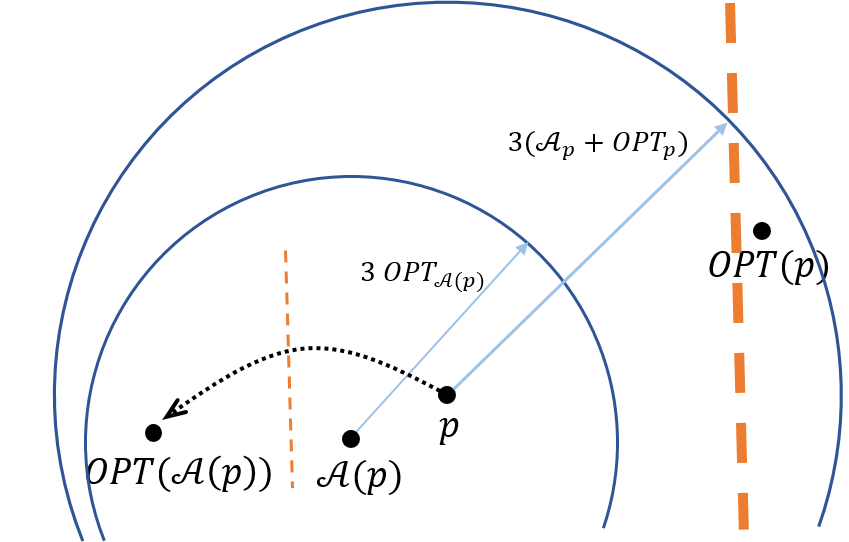
This essentially concludes the case where $p$ is not badly cut. When it is badly cut, the decomposition $𝒟$ approximates its distances poorly; however, this happens with tiny probability, and we can afford to move $p$ to $𝒜(p)$ (charging this movement to $b_1(p,\epsilon )$). A case analysis, similar to the previous one, then shows that the detour between $𝒜(p)$ to OPT can be charged to $b_2(p,\epsilon )$ and $b_3(p,\epsilon )$.

In the remainder of this section, we show how to remove some centers from the optimal solution (to then add the badly cut centers of $𝒜$), then prove the structure theorem that shows the existence of a solution satisfying (1) and (2). We explain in Section 3.4 the dynamic program that relies on this structure theorem and enables the computation of a good approximation, to conclude the proof of Theorem 2.

We consider the mapping of the centers of OPT to $𝒜$ defined as follows: for any $f\in \text{OPT}$, let $𝒜(f)$ denote the center of $𝒜$ that is the closest to $f$. Recall that for a client $c$, $𝒜(c)$ is the center serving $c$ in $𝒜$.

For any center $\mathrm{\ell }$ of $𝒜$, define $\psi (\mathrm{\ell })$ to be the set of centers of OPT that are mapped to $\mathrm{\ell }$, namely, $\psi (\mathrm{\ell })=\{f\in \text{OPT}\mid 𝒜(f)=\mathrm{\ell }\}$. Define ${𝒜}^1$ to be the set of centers $\mathrm{\ell }$ of $𝒜$ for which there exists a unique $f\in \text{OPT}$ such that $𝒜(f)=\mathrm{\ell }$, namely ${𝒜}^1=\{\mathrm{\ell }\in 𝒜\mid |\psi (\mathrm{\ell })|=1\}$. Let ${𝒜}^0=\{\mathrm{\ell }\in 𝒜\mid |\psi (\mathrm{\ell })|=0\}$, and ${𝒜}^{\ge 2}=𝒜\setminus ({𝒜}^1\cup {𝒜}^0)$. Similarly, define ${\text{OPT}}^1=\{f\in \text{OPT}\mid 𝒜(f)\in {𝒜}^1\}$ and ${\text{OPT}}^{\ge 2}=\{f\in \text{OPT}\mid 𝒜(f)\in {𝒜}^{\ge 2}\}$. Note that $|{\text{OPT}}^{\ge 2}|=|{𝒜}^0|+|{𝒜}^{\ge 2}|$, since $|{\text{OPT}}^1|=|{𝒜}^1|$ and, w.l.o.g., $|\text{OPT}|=|𝒜|=k$.

As shown in [13], one can remove some of the centers from ${\text{OPT}}^{\ge 2}$ to obtain the following result:

Furthermore, we transform the input set $P$ to give it more structure, as follows. Given a randomized hierarchical decomposition $𝒟$ and a solution $𝒜$, we define the set $\tilde{P}$ as follows. For every point $p$,

We note that $\tilde{P}:=\{\tilde{p}:p\in P\}$ is a random variable that depends on the randomness of $𝒟$.

Using Lemma 9, we can now show the existence of a near-optimal portal-respecting solution. Let $𝒜$ be a fixed solution, and ${\text{OPT}}^{\prime }$ the solution from Lemma 9 for $P$. Let $𝒟$ be a randomized hierarchical decomposition, and $B_{𝒟}$ be the set of centers of $𝒜$ that are badly cut w.r.t. ${\text{OPT}}^{\prime }$, i.e., $c\in B_{𝒟}$ when the ball $B(c,3{\text{OPT}}_c^{\prime })$ is cut at some level greater than $\log (3{\text{OPT}}_c^{\prime })+\tau (\epsilon ,d)$.

As explained in the introduction, we will use those properties as follows: a standard dynamic program will compute the best portal-respecting solution that minimizes $\widetilde{\mathrm{cost}}(P,𝒮):={\sum }_p{(\mathrm{dist}(p,\tilde{p})+\mathrm{dist}(\tilde{p},𝒮))}^2$. Making the solution portal-respecting incurs an error $\epsilon 2^i$ for two points cut at level $i$: Property 3 therefore bounds this error by $b(p,\epsilon )$. Property 1 of Definition 10 ensures that the total budget is bounded, and Property 2 relates $\widetilde{\mathrm{cost}}$ to $\mathrm{cost}$.

Our main structural theorem for $k$-means in low dimension is the following:

The rest of the paper is dedicated to the proof of this theorem.

References

- [1] Fateme Abbasi, Sandip Banerjee, Jaroslaw Byrka, Parinya Chalermsook, Ameet Gadekar, Kamyar Khodamoradi, Dániel Marx, Roohani Sharma, and Joachim Spoerhase. Parameterized approximation schemes for clustering with general norm objectives. In 64th IEEE Annual Symposium on Foundations of Computer Science, FOCS 2023, Santa Cruz, CA, USA, November 6-9, 2023, pages 1377–1399. IEEE, 2023. doi:10.1109/FOCS57990.2023.00085.
- [2] Enver Aman, Karthik C. S., and Sharath Punna. On connections between k-coloring and Euclidean k-means. In Timothy M. Chan, Johannes Fischer, John Iacono, and Grzegorz Herman, editors, 32nd Annual European Symposium on Algorithms, ESA 2024, September 2-4, 2024, Royal Holloway, London, United Kingdom, volume 308 of LIPIcs, pages 9:1–9:18. Schloss Dagstuhl – Leibniz-Zentrum für Informatik, 2024. doi:10.4230/LIPIcs.ESA.2024.9.
- [3] Sanjeev Arora. Polynomial time approximation schemes for Euclidean TSP and other geometric problems. In 37th Annual Symposium on Foundations of Computer Science, FOCS ’96, Burlington, Vermont, USA, 14-16 October, 1996, pages 2–11. IEEE Computer Society, 1996. doi:10.1109/SFCS.1996.548458.
- [4] Sanjeev Arora. Polynomial time approximation schemes for Euclidean traveling salesman and other geometric problems. J. ACM, 45(5):753–782, 1998. doi:10.1145/290179.290180.
- [5] Sanjeev Arora, Prabhakar Raghavan, and Satish Rao. Approximation schemes for Euclidean k-medians and related problems. In Jeffrey Scott Vitter, editor, Proceedings of the Thirtieth Annual ACM Symposium on the Theory of Computing, Dallas, Texas, USA, May 23-26, 1998, pages 106–113. ACM, 1998. doi:10.1145/276698.276718.
- [6] Pranjal Awasthi, Moses Charikar, Ravishankar Krishnaswamy, and Ali Kemal Sinop. The hardness of approximation of Euclidean k-means. In Lars Arge and János Pach, editors, 31st International Symposium on Computational Geometry, SoCG 2015, June 22-25, 2015, Eindhoven, The Netherlands, volume 34 of LIPIcs, pages 754–767. Schloss Dagstuhl – Leibniz-Zentrum für Informatik, 2015. doi:10.4230/LIPIcs.SOCG.2015.754.
- [7] Yair Bartal and Lee-Ad Gottlieb. A linear time approximation scheme for Euclidean TSP. In 54th Annual IEEE Symposium on Foundations of Computer Science, FOCS 2013, 26-29 October, 2013, Berkeley, CA, USA, pages 698–706. IEEE Computer Society, 2013. doi:10.1109/FOCS.2013.80.
- [8] Vladimir Braverman, Gereon Frahling, Harry Lang, Christian Sohler, and Lin F. Yang. Clustering high dimensional dynamic data streams. In Doina Precup and Yee Whye Teh, editors, Proceedings of the 34th International Conference on Machine Learning, ICML 2017, Sydney, NSW, Australia, 6-11 August 2017, volume 70 of Proceedings of Machine Learning Research, pages 576–585. PMLR, 2017. URL: http://proceedings.mlr.press/v70/braverman17a.html.
- [9] Moses Charikar, Vincent Cohen-Addad, Ruiquan Gao, Fabrizio Grandoni, Euiwoong Lee, and Ernest van Wijland. An improved greedy approximation for (metric) k-means. In 66th IEEE Annual Symposium on Foundations of Computer Science, FOCS 2025, Sydney, Australia, December 14-17, 2025, pages 233–240. IEEE, 2025. doi:10.1109/FOCS63196.2025.00016.
- [10] Vincent Cohen-Addad. A fast approximation scheme for low-dimensional k-means. In Artur Czumaj, editor, Proceedings of the Twenty-Ninth Annual ACM-SIAM Symposium on Discrete Algorithms, SODA 2018, New Orleans, LA, USA, January 7-10, 2018, pages 430–440. SIAM, 2018. doi:10.1137/1.9781611975031.29.
- [11] Vincent Cohen-Addad, Arnaud de Mesmay, Eva Rotenberg, and Alan Roytman. The bane of low-dimensionality clustering. In Proceedings of the 2018 Annual ACM-SIAM Symposium on Discrete Algorithms (SODA), 2018. doi:10.1137/1.9781611975031.30.
- [12] Vincent Cohen-Addad, Alessandro Epasto, Silvio Lattanzi, Vahab Mirrokni, Andres Muñoz Medina, David Saulpic, Chris Schwiegelshohn, and Sergei Vassilvitskii. Scalable differentially private clustering via hierarchically separated trees. In Aidong Zhang and Huzefa Rangwala, editors, KDD ’22: The 28th ACM SIGKDD Conference on Knowledge Discovery and Data Mining, Washington, DC, USA, August 14 - 18, 2022, pages 221–230. ACM, 2022. doi:10.1145/3534678.3539409.
- [13] Vincent Cohen-Addad, Andreas Emil Feldmann, and David Saulpic. Near-linear time approximation schemes for clustering in doubling metrics. J. ACM, 68(6):44:1–44:34, 2021. doi:10.1145/3477541.
- [14] Vincent Cohen-Addad, Andreas Emil Feldmann, and David Saulpic. Near-linear time approximation schemes for clustering in doubling metrics. In J. ACM, volume 68, 2021. doi:10.1145/3477541.
- [15] Vincent Cohen-Addad, Fabrizio Grandoni, Euiwoong Lee, Chris Schwiegelshohn, and Ola Svensson. A (2+)-approximation algorithm for metric k-median. In Michal Koucký and Nikhil Bansal, editors, Proceedings of the 57th Annual ACM Symposium on Theory of Computing, STOC 2025, Prague, Czechia, June 23-27, 2025, pages 615–624. ACM, 2025. doi:10.1145/3717823.3718299.
- [16] Vincent Cohen-Addad, Anupam Gupta, Amit Kumar, Euiwoong Lee, and Jason Li. Tight FPT approximations for k-median and k-means. In Christel Baier, Ioannis Chatzigiannakis, Paola Flocchini, and Stefano Leonardi, editors, 46th International Colloquium on Automata, Languages, and Programming, ICALP 2019, July 9-12, 2019, Patras, Greece, volume 132 of LIPIcs, pages 42:1–42:14. Schloss Dagstuhl – Leibniz-Zentrum für Informatik, 2019. doi:10.4230/LIPIcs.ICALP.2019.42.
- [17] Vincent Cohen-Addad and Karthik C. S. Inapproximability of clustering in lp metrics. In David Zuckerman, editor, 60th IEEE Annual Symposium on Foundations of Computer Science, FOCS 2019, Baltimore, Maryland, USA, November 9-12, 2019, pages 519–539. IEEE Computer Society, 2019. doi:10.1109/FOCS.2019.00040.
- [18] Vincent Cohen-Addad, Karthik C. S., and Euiwoong Lee. On approximability of clustering problems without candidate centers. In Dániel Marx, editor, Proceedings of the 2021 ACM-SIAM Symposium on Discrete Algorithms, SODA 2021, Virtual Conference, January 10 - 13, 2021, pages 2635–2648. SIAM, 2021. doi:10.1137/1.9781611976465.156.
- [19] Vincent Cohen-Addad, Karthik C. S., and Euiwoong Lee. Johnson coverage hypothesis: Inapproximability of k-means and k-median in -metrics. In Joseph (Seffi) Naor and Niv Buchbinder, editors, Proceedings of the 2022 ACM-SIAM Symposium on Discrete Algorithms, SODA 2022, Virtual Conference / Alexandria, VA, USA, January 9 - 12, 2022, pages 1493–1530. SIAM, 2022. doi:10.1137/1.9781611977073.63.
- [20] Vincent Cohen-Addad, Philip N. Klein, and Claire Mathieu. Local search yields approximation schemes for k-means and k-median in Euclidean and minor-free metrics. SIAM J. Comput., 48(2):644–667, 2019. doi:10.1137/17M112717X.
- [21] Vincent Cohen-Addad, Silvio Lattanzi, Ashkan Norouzi-Fard, Christian Sohler, and Ola Svensson. Fast and accurate $k$-means++ via rejection sampling. In Hugo Larochelle, Marc’Aurelio Ranzato, Raia Hadsell, Maria-Florina Balcan, and Hsuan-Tien Lin, editors, Advances in Neural Information Processing Systems 33: Annual Conference on Neural Information Processing Systems 2020, NeurIPS 2020, December 6-12, 2020, virtual, 2020. URL: https://proceedings.neurips.cc/paper/2020/hash/babcff88f8be8c4795bd6f0f8cccca61-Abstract.html.
- [22] Vincent Cohen-Addad, David Saulpic, and Chris Schwiegelshohn. A new coreset framework for clustering. In Samir Khuller and Virginia Vassilevska Williams, editors, STOC ’21: 53rd Annual ACM SIGACT Symposium on Theory of Computing, Virtual Event, Italy, June 21-25, 2021, pages 169–182. ACM, 2021. doi:10.1145/3406325.3451022.
- [23] Sanjoy Dasgupta and Yoav Freund. Random projection trees for vector quantization. IEEE Transactions on Information Theory, 55(7):3229–3242, 2009. doi:10.1109/TIT.2009.2021326.
- [24] Mark de Berg, Hans L. Bodlaender, Sándor Kisfaludi-Bak, Dániel Marx, and Tom C. van der Zanden. A framework for exponential-time-hypothesis-tight algorithms and lower bounds in geometric intersection graphs. SIAM J. Comput., 49(6):1291–1331, 2020. doi:10.1137/20M1320870.
- [25] Irit Dinur. Mildly exponential reduction from gap 3sat to polynomial-gap label-cover. Electron. Colloquium Comput. Complex., TR16-128, 2016. URL: https://eccc.weizmann.ac.il/report/2016/128.
- [26] Fedor V. Fomin, Petr A. Golovach, and Kirill Simonov. Parameterized k-clustering: Tractability island. J. Comput. Syst. Sci., 117:50–74, 2021. doi:10.1016/J.JCSS.2020.10.005.
- [27] Zachary Friggstad, Mohsen Rezapour, and Mohammad R. Salavatipour. Local search yields a PTAS for k-means in doubling metrics. SIAM J. Comput., 48(2):452–480, 2019. doi:10.1137/17M1127181.
- [28] Sudipto Guha and Samir Khuller. Greedy strikes back: Improved facility location algorithms. J. Algorithms, 31(1):228–248, 1999. doi:10.1006/jagm.1998.0993.
- [29] S Louis Hakimi. Optimum distribution of switching centers in a communication network and some related graph theoretic problems. Operations research, 13(3):462–475, 1965.
- [30] Sariel Har-Peled. Geometric approximation algorithms. Number 173 in Mathematical Surveys and Monographs. American Mathematical Soc., 2011.
- [31] Mary Inaba, Naoki Katoh, and Hiroshi Imai. Applications of weighted voronoi diagrams and randomization to variance-based k-clustering (extended abstract). In Proceedings of the Tenth Annual Symposium on Computational Geometry, Stony Brook, New York, USA, June 6-8, 1994, pages 332–339, 1994. doi:10.1145/177424.178042.
- [32] Kamal Jain, Mohammad Mahdian, and Amin Saberi. A new greedy approach for facility location problems. In Proceedings on 34th Annual ACM Symposium on Theory of Computing, May 19-21, 2002, Montréal, Québec, Canada, pages 731–740, 2002. doi:10.1145/509907.510012.
- [33] Kamal Jain and Vijay V. Vazirani. Approximation algorithms for metric facility location and k-median problems using the primal-dual schema and lagrangian relaxation. J. ACM, 48(2):274–296, 2001. doi:10.1145/375827.375845.
- [34] Sándor Kisfaludi-Bak, Jesper Nederlof, and Karol Wegrzycki. A gap-ETH-tight approximation scheme for Euclidean TSP. Journal of the ACM, 72(6):1–48, 2025.
- [35] Stavros G. Kolliopoulos and Satish Rao. A nearly linear-time approximation scheme for the Euclidean k-median problem. SIAM J. Comput., 37(3):757–782, 2007. doi:10.1137/S0097539702404055.
- [36] Alfred A Kuehn and Michael J Hamburger. A heuristic program for locating warehouses. Management science, 9(4):643–666, 1963.
- [37] Euiwoong Lee, Melanie Schmidt, and John Wright. Improved and simplified inapproximability for k-means. Inf. Process. Lett., 120:40–43, 2017. doi:10.1016/j.ipl.2016.11.009.
- [38] Shi Li and Ola Svensson. Approximating k-median via pseudo-approximation. SIAM J. Comput., 45(2):530–547, 2016. doi:10.1137/130938645.
- [39] Stuart Lloyd. Least squares quantization in pcm. IEEE transactions on information theory, 28(2):129–137, 1982. doi:10.1109/TIT.1982.1056489.
- [40] Meena Mahajan, Prajakta Nimbhorkar, and Kasturi R. Varadarajan. The planar k-means problem is np-hard. Theor. Comput. Sci., 442:13–21, 2012. doi:10.1016/J.TCS.2010.05.034.
- [41] Konstantin Makarychev, Yury Makarychev, and Ilya P. Razenshteyn. Performance of johnson-lindenstrauss transform for k-means and k-medians clustering. In Proceedings of the 51st Annual ACM SIGACT Symposium on Theory of Computing, STOC 2019, Phoenix, AZ, USA, June 23-26, 2019, pages 1027–1038, 2019. doi:10.1145/3313276.3316350.
- [42] Pasin Manurangsi and Prasad Raghavendra. A birthday repetition theorem and complexity of approximating dense csps. In Ioannis Chatzigiannakis, Piotr Indyk, Fabian Kuhn, and Anca Muscholl, editors, 44th International Colloquium on Automata, Languages, and Programming, ICALP 2017, July 10-14, 2017, Warsaw, Poland, volume 80 of LIPIcs, pages 78:1–78:15. Schloss Dagstuhl – Leibniz-Zentrum für Informatik, 2017. doi:10.4230/LIPIcs.ICALP.2017.78.
- [43] Jirí Matousek. On approximate geometric k-clustering. Discret. Comput. Geom., 24(1):61–84, 2000. doi:10.1007/s004540010019.
- [44] Nimrod Megiddo and Kenneth J Supowit. On the complexity of some common geometric location problems. SIAM journal on computing, 13(1):182–196, 1984. doi:10.1137/0213014.
- [45] Satish B Rao and Warren D Smith. Approximating geometrical graphs via “spanners” and “banyans”. In Proceedings of the thirtieth annual ACM symposium on Theory of computing, pages 540–550, 1998.
- [46] John Fred Stollsteimer. The effect of technical change and output expansion on the optimum number, size, and location of pear marketing facilities in a California pear producing region. University of California, Berkeley, 1961.