A Free Lunch: Manifolds of Positive Reach Can Be Smoothed Without Decreasing the Reach

Abstract
Assumptions on the reach are crucial for ensuring the correctness of many geometric and topological algorithms, including triangulation, manifold reconstruction and learning, homotopy reconstruction, and methods for estimating curvature or reach. However, these assumptions are often coupled with the requirement that the manifold be smooth, typically at least .
In this paper, we prove that any manifold with positive reach can be approximated arbitrarily well by a manifold without significantly reducing the reach. More precisely, given a manifold with reach , we construct a manifold that is -close to it in the sense (both the manifold and its tangent spaces are close), and has reach at least . The proof employs techniques from differential topology – partitions of unity and smoothing using convolution kernels.
This result implies that nearly all theorems established for or manifolds with a certain reach naturally extend to manifolds with the same reach, even if they are not , for free!
Keywords and phrases:
Reach, Manifolds, Smoothing, Differentiability, Differential topologyFunding:
Hana Dal Poz Kouřimská: Supported by the DFG project No. 524578210.Copyright and License:
![[Uncaptioned image]](x1.png) © Hana Dal Poz Kouřimská, André Lieutier, and Mathijs Wintraecken; licensed under Creative Commons License CC-BY 4.0
© Hana Dal Poz Kouřimská, André Lieutier, and Mathijs Wintraecken; licensed under Creative Commons License CC-BY 4.0
2012 ACM Subject Classification:
Theory of computation Computational geometryAcknowledgements:
We thank Jean-Daniel Boissonnat for discussion. We would also like to acknowledge the organizers of the workshop on “Algorithms for the Medial Axis”, and Erin Chambers in particular, for giving an impulse to this research. We further thank Victor Bangert for encouragement.Editors:
Hee-Kap Ahn, Michael Hoffmann, and Amir NayyeriSeries and Publisher:
 Leibniz International Proceedings in Informatics, Schloss Dagstuhl – Leibniz-Zentrum für Informatik
1 Introduction
What is the reach?
The reach of a set is a number that captures the geometric properties of its shape. Roughly speaking, it provides a bound on the set’s curvature and quantifies how far apart different parts of the set are from each other. As a key descriptor of a shape’s complexity, the reach plays a crucial role as an assumption in many geometric and topological algorithms.
Formally, the reach of a (closed) set is the minimum of the distance between and its medial axis, that is, the set of points in for which the closest point in is not unique. We illustrate these notions in Figure 1.

The early history of the reach.
The reach was first introduced by Federer in [20]. Notably, earlier work by Erdős explored what we now refer to as the medial axis, although it did not address the reach itself [18, 19]. While Erdős studied the medial axis and Federer considered its complement, the term “medial axis” itself was coined only later, by Blum [12]. A related notion, the cut locus in Riemannian geometry, has a significantly longer history, with its origins traced to the work of Poincaré [34], Whitehead [38], and Myers [31, 32]111See [35] for a nice overview of the early history of the cut locus..
Due to their wide applicability, these concepts have been reintroduced multiple times. For instance, the (closure of) medial axis was reintroduced as the central set by Milman and Waksman [30], its complement as the unique footprint set by Kleinjohann [25], and the reach was referred to as the condition number by Niyogi, Smale, and Weinberger [33].
The reach and differentiability.
In [20], Federer established that the reach is stable under -diffeomorphisms of the ambient space. Here, denotes a map whose derivative is Lipschitz, and by a -diffeomorphism, we mean that both the diffeomorphism and its inverse are . Federer also mentioned, without extensive detail [20, Remark 4.20], that the graph of a function has positive reach if and only if the function itself is . Lytchak [27, 28] later proved that a topological submanifold of the Euclidean space without boundary has positive reach if and only if it is a -submanifold. A quantified version of this statement can be found in [26].
The reach in computational geometry and topology, and manifold learning.
The reach encapsulates the geometric complexity of a shape in a single non-negative value, making it a crucial assumption for ensuring the correctness of many geometric and topological algorithms. Several key classes of algorithms that depend on reach assumptions include:
All these algorithms have as input a point cloud queried from a manifold. Their output, and its correctness, varies:
-
Triangulation algorithms produce as output a simplicial complex – often, but not always a variant of the Delaunay triangulation. Such algorithms are perceived as correct if the output complex is (piecewise linearly) homeomorphic to the underlying manifold.
-
Manifold learning algorithms output a description of an approximation of the given manifold – for example as the zero set of a function or a projection operator. Such algorithms are correct if the output approximation is homeomorphic to the underlying manifold and sufficiently geometrically close to it.
-
Homotopy inference algorithms output a simplicial complex, which is correct if it is homotopy equivalent to the underlying manifold.
For the success of these algorithms, it is essential to provide criteria that guarantee their correctness and quality. Such criteria are often formulated using the reach of the manifold.
In addition, reach estimation in and by itself is an important topic in inference (see for example [1, 2, 11]). The typical setting for this type of problems involves a point cloud, which is drawn from a probability measure whose support is a manifold satisfying a regularity condition. Such condition can, for example, be a guarantee that the reach of the manifold in question is larger than some (very small positive) constant. The goal is to estimate the actual reach of the manifold, with a guaranteed precision margin.
Most of the aforementioned works assume that the manifold in question is at least , in addition to having positive reach. This assumption is often made because it allows the use of the full machinery of differential and Riemannian geometry. For instance, the second fundamental form is always well-defined in the setting [16, 17]. Yet, this condition is not entirely natural. Manifolds with positive reach are indeed at least , see [26, 27, 28], and by Rademacher’s theorem [21], they are almost everywhere, but not necessarily everywhere.
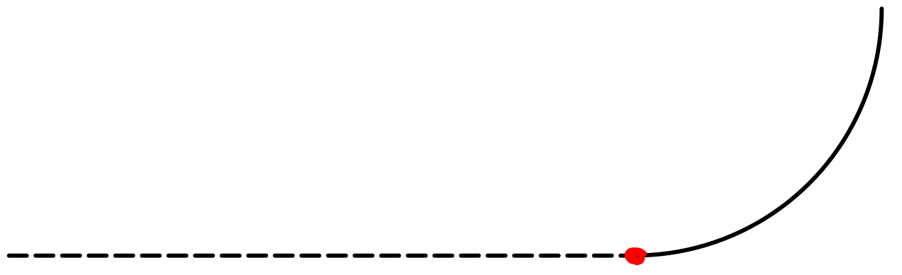
On the other hand, requiring the manifold in question to be is quite natural, as it encompasses many configurations commonly found in modern modeling software, such as computer-aided design (CAD). This is because the majority of manufactured objects can be modeled as surfaces: For instance, consider a line segment and a circular arc intersecting at a point where their tangents coincide, as illustrated in Figure 2. This configuration has positive reach but is only .
As a consequence of the results presented in this article (primarily Theorem 1), all aforementioned results can be extended from manifolds with positive reach to arbitrary manifolds with positive reach; hence the paper title.
Our settings.
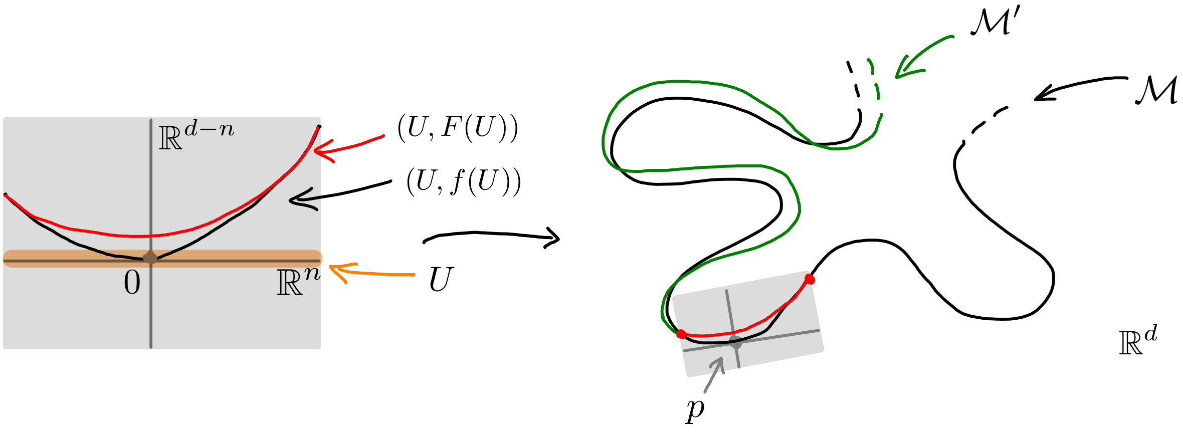
In this work, we identify an embedded manifold locally (in a neighborhood of a point ) as a graph of a map from its tangent space to its normal space at . This approach, which we illustrate in Figure 3, allows us to compare homeomorphic manifolds ( and in Figure 3), embedded in Euclidean space of the same dimension, by comparing their corresponding maps and their derivatives ( and in the figure). We say that two such manifolds are close in the sense, if, roughly speaking, both the manifolds and their tangent spaces are close. Formally, this is a condition on the corresponding maps and , and we explain it in Definition 11.
Throughout the paper, we denote the dimension of the manifolds and by , and the dimension of the ambient Euclidean space by .

Our contribution.
Our main contribution is the following statement:
Theorem 1.
Let be a compact manifold of (positive) reach , and . Then there exists a manifold such that:
-
and are -close as embedded manifolds in the sense.
-
The reach of satisfies .
Remark 2.
We can either remove the compactness assumption (because we only need a locally finite cover in the proof of the theorem) or we can assume that the reach is not decreased by . More precisely, if the manifold is compact, we can increase the reach of the manifold by scaling it by a factor , and achieve . However, this may increase the distance between and in the sense (by ).
In addition, our result can be restated in terms of density in the space of submanifolds:
Corollary 3.
The space of embedded submanifolds of with reach is dense (in the topology) in the space of embedded submanifolds of with reach .
This reformulation of the main theorem stands in a long line of density results from functional analysis and differential topology222We refer to Chapter 2 of [24] for an extensive overview.. Such results have been widely used to extend results from a smaller to a larger class of functions, without any extra effort. Hence, our result establishes a new link between computational geometry, topology, and manifold learning on the one hand, and functional analysis and differential topology on the other.
The main results from this paper might appear trivial to experts in differential topology at first glance: It is well known that Lipschitz functions can be smoothed while preserving the Lipschitz bounds of both the function and its derivative – a fact that is straightforward and proved succinctly in Lemmas 15 and 16. However, this observation alone is far from sufficient to achieve the main result of the paper.
Outline.
The structure of the paper closely follows the different steps in the proof of Theorem 1. Let us provide you with an outlook:
Step 1: We start with a compact submanifold of of positive reach.
For each point , we can find a neighbourhood in which is a graph of a function from the (affine) tangent to the normal space at .
Since the reach of is positive, this function is , and we use the bound on the Lipschitz constant of its derivative to control the angles between nearby tangent spaces.
We fix an and select a sample of points whose neighbourhoods cover (see Figure 4). We only work with one neighbourhood at a time.

Step 2: We identify the point with , and the tangent and normal spaces and with the first and last coordinates of , respectively. Following this identification, we denote the map describing by , and its domain by .
Our first goal is to smooth in a neighbourhood of . We split into three regions: a neighbourhood of , a region covering the vicinity of , and a transition region in between. We then use kernel-based smoothing to define a function
that is smooth in and equals in (see Figure 5). To achieve this, we employ a partition of unity function. We revise the background on smoothing and partitions of unity in Section 2.1. These techniques allow us to control the Lipschitz constant of and its derivative, on which we give explicit bounds in Sections 3.1 and 3.2. We use operator norms to formulate these bounds. The background on operator norms is also presented in Section 2.1.

Step 3:
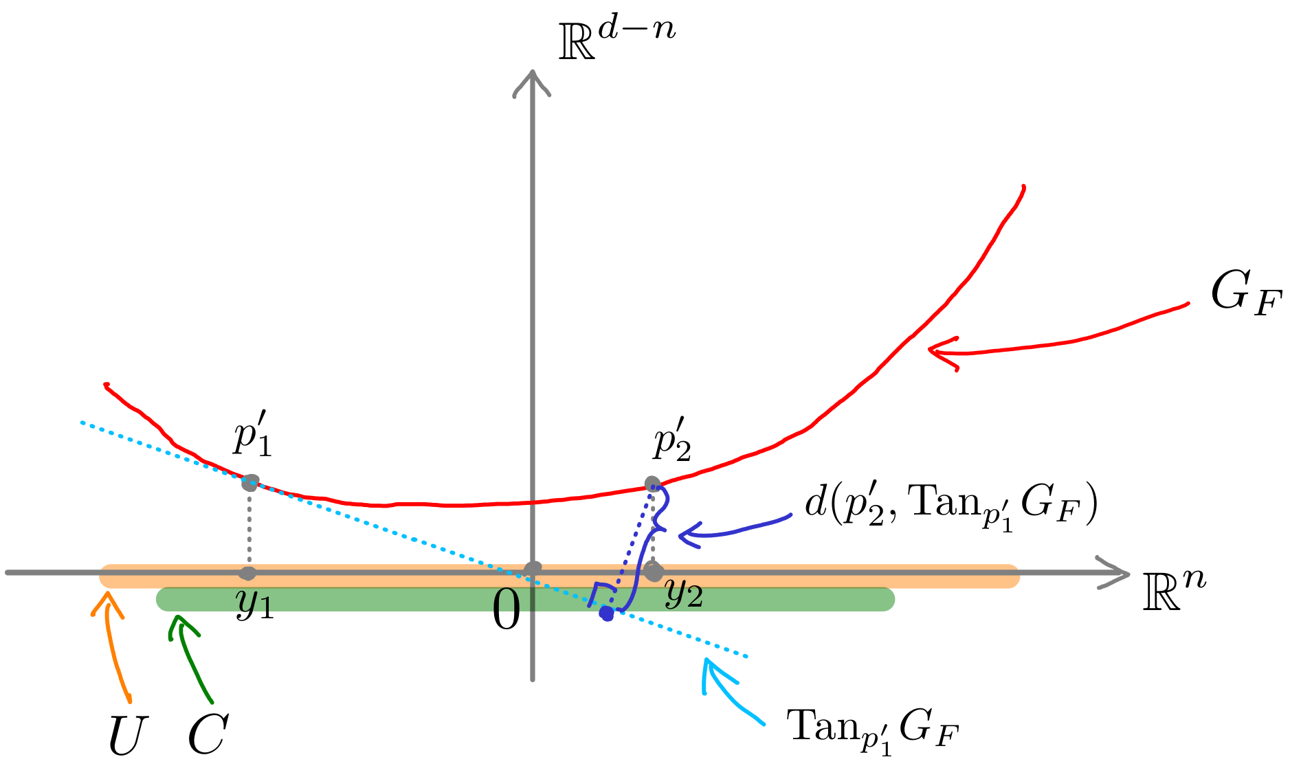
We perform surgery on the manifold , and replace the graph of by the graph of . We abuse notation and call this manifold , although it is “only” smooth in a neighbourhood of the point for now. Then we estimate the reach of . To this end, we leverage a result by Federer, which characterizes the reach of a manifold through the distance from a point on it to the affine tangent space of another point on it.
We pick two points in and investigate the distance from to the affine tangent space of . It turns out that bounding this distance is straightforward when does not lie in the graph of . In the other case, we establish the bound using the relationship between the functions and , and the Lipschitz constants of and its derivative. We cover these results in Section 3.3.
Step 4:
We repeat Steps 2 and 3 iteratively for each point of our sample, until we have smoothed the whole of . The process is illustrated in Figure 6. In each iteration, we have a one-parameter freedom in the choice of the smoothing kernel.
In this final step of the proof, we show that both the point sample and the smoothing kernels can be chosen in such a way that at the end, the smooth manifold satisfies the conditions of Theorem 1. This final step is described in Section 4.
We indicate all the results in the paper that are (most probably) well known to experts in differential topology as “Folklore”. We provide proofs of these statements,as well as the proofs of all our statements except the main theorem, in the full version of this article.
2 Preliminaries
We assume that the reader is reasonably familiar with sets of positive reach. Furthermore, we recall a characterization of the reach given by Federer [20] and results on Lipschitz-continuity of maps from a tangent space into a normal space of a manifold in the full version of this article.
2.1 Results from differential topology
In this section we recall three elementary tools from differential topology: partition of unity functions, the smoothing process, and operator norms. We adopt the formulation and notation used by Hirsch [24, Chapter 2].
Partition of unity functions
Partition of unity functions allow us to localize constructions and proofs in differential topology. They are defined as follows:
Definition 4.
Let be a manifold, with , and , with an index set , an open cover of . A partition of unity subordinate to is a family of maps , , with the following properties:
-
For every , the support333The support of a function is the closure of the set . of is contained in the set .
-
The collection of the supports of is locally finite.
-
The maps sum to the function that is identically equal to , that is,
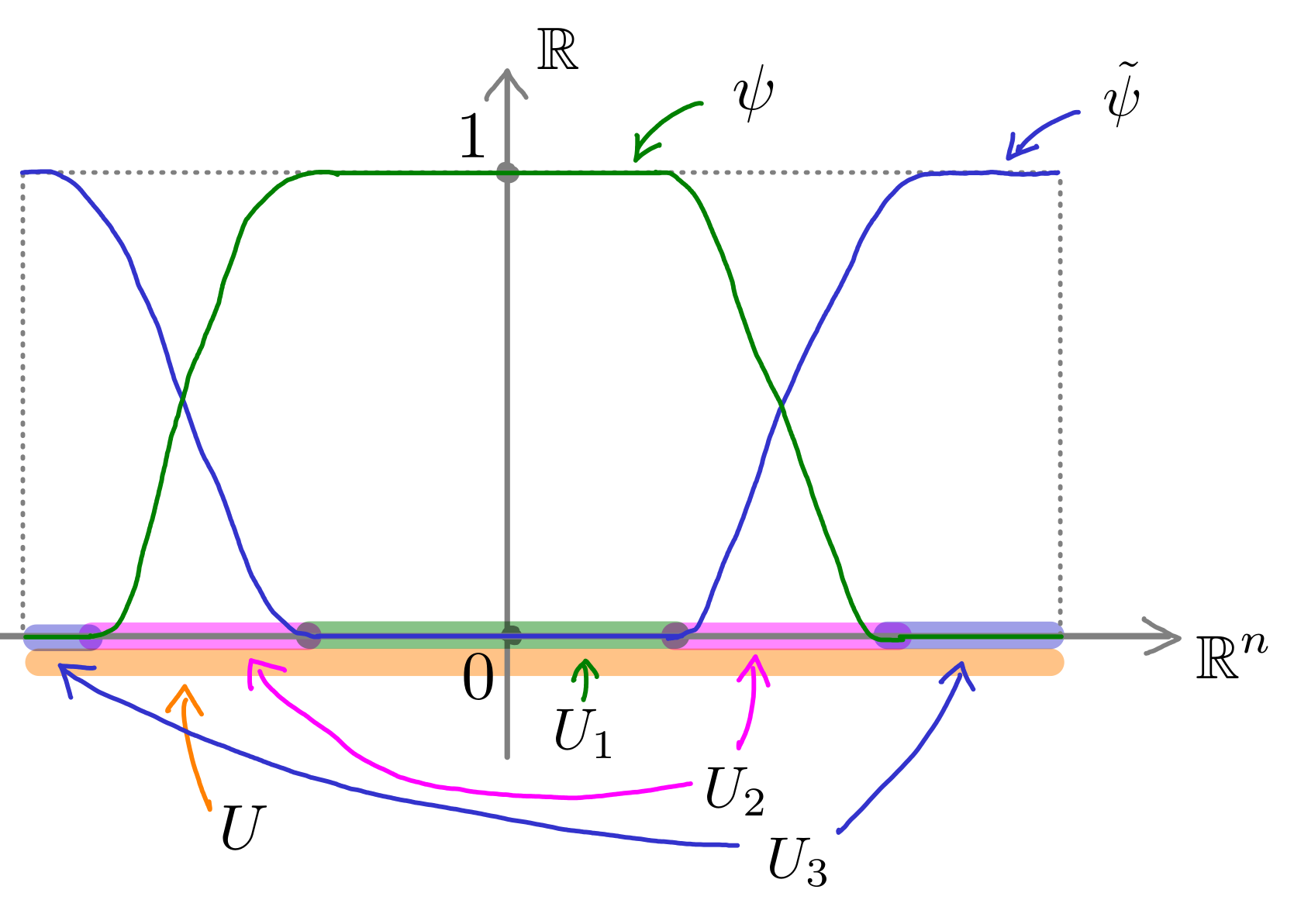
We illustrate the concept for our setting in Figure 7. We can find a partition of unity for any open cover:
Theorem 5 (Theorem 2.1 of [24]).
Let be a manifold with . Every open cover of has a subordinate partition of unity.
Kernel smoothing
Kernel smoothing is, broadly speaking, a process that averages a map using a kernel function, making the result at least as smooth as the kernel itself. The kernel is defined as follows:
Definition 6 (Smoothing kernel).
A (smooth) map is called a convolution or a smoothing kernel if it is non-negative, has compact support, and .
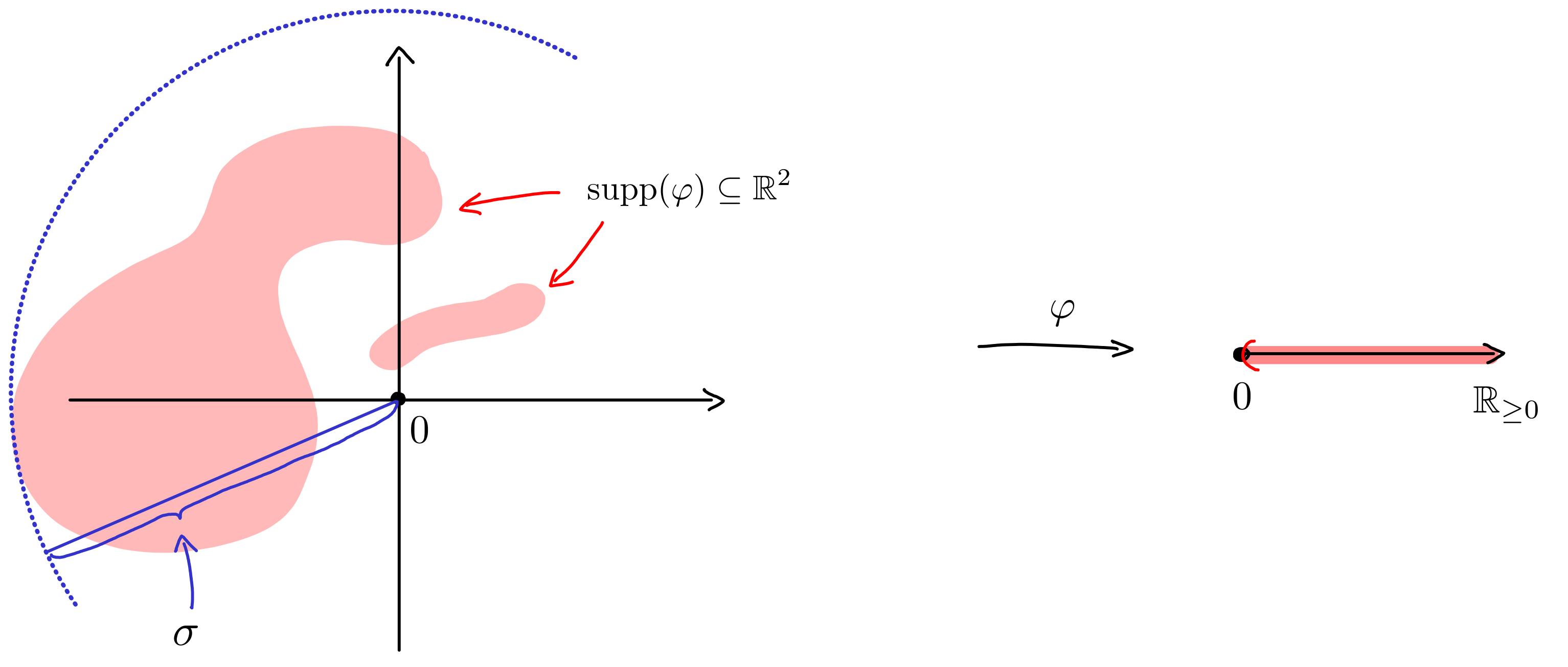
The support radius of the smoothing kernel is the smallest value , for which the support of is contained in the closed ball of radius centred at the origin:
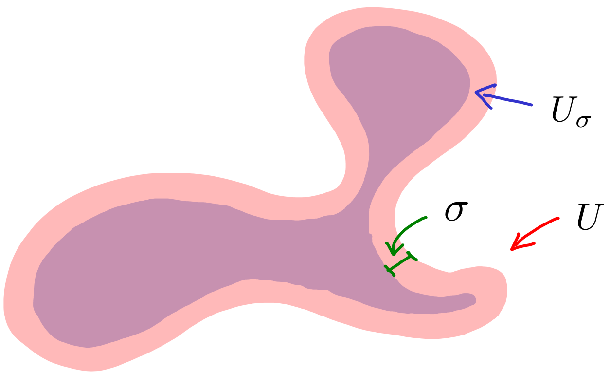
We illustrate the smoothing radius in Figure 8.
Smoothing relies on neighbourhoods, determined by the support radius of the kernel. For smoothing of a map on a given set to be well-defined, the map itself must be well-defined on a sufficiently thick neighborhood surrounding the set. Consequently, it is sometimes necessary to shrink the domain of the map where the smoothing will be applied:
Definition 7.
Consider a smoothing kernel with support radius . Given an open set , the shrinking of is defined as
The smoothing process, or in other words, the convolution, is carried out through integration:
Definition 8 (Convolution).
Let be a smoothing kernel with support radius , an open set, and a continuous map. The convolution of by is the map
Smoothing improves the smoothness of the map, and commutes with differentiation:
Theorem 9 ([24, Theorem 2.3 (a) and (b)]).
Let be a smoothing kernel with support radius , an open set and a continuous map. The convolution has the following properties:
-
If is , with , then so is , and for each finite ,
on .
-
If is , with , then so is , and for each finite ,
Operator norms
The last result we need is the convergence of smoothed maps to the original map. We consider convergence of the map itself as well as its first derivatives with respect to the so-called norm. We define this norm in two steps:
Definition 10.
The norm of a -linear map
is defined as
Consider a map , and its th order derivative . For , the map is an -linear map at each point , and we use the above definition to measure the norm of at . For , the notation should be understood as .
Definition 11 ( norm).
Let be a map, an open set, and any subset of . The norm of on is defined as
We can now define the convergence we will use:
Theorem 12 ([24, Theorem 2.3 (c)]).
Let be an open set with a compact subset , and a map, with . For any there exists a value such that , and any smoothing kernel with support radius satisfies
Remark 13.
The operator -norm of a matrix is defined as
where denotes the usual Euclidean (-)norm.
For the first derivative of a function , evaluated at a point , the norm from Definition 10 coincides with the operator -norm, that is, . In particular,
In this paper, we primarily focus on the case where , as estimating the first derivative proves to be the main challenge in our proofs. Consequently, much of our work involves dealing with operator 2-norms.
In addition, we often make a choice of the map on which we perform the smoothing. The lemma below implies that our choice does not depend on the map itself, but only on its Lipschitz constant.
Lemma 14 (Folklore).
We adapt the settings from Theorem 12. If the map is -Lipschitz, then for any point and it holds that . As a consequence,
3 On the control over Lipschitz constants while smoothing and using partition of unity functions
This section consists of three parts, in which we
-
recall that smoothing by convolution does not affect Lipschitz constants;
-
set the stage to define the function that locally describes our smoothed manifold , and determine the Lipschitz constant of and its derivative;
-
establish two bounds on the distance between the affine tangent space of a point on the graph of , and another point in .
3.1 Lipschitz constants for smoothings by convolution
In this section we focus on Lipschitz constants. To this end, we denote the Lipschitz constant of a function by . We recall that a function is Lipschitz with constant if for all points
| (1) |
Similarly, if is differentiable, the derivative of is Lipschitz with constant if for all points
| (2) |
We first recall that smoothing does not influence the Lipschitz constant of a function or its derivative.
The result of the convolution of a function by a kernel is just a barycenter of translates of . Since the minimal Lipschitz constant satisfied by a function defines a semi-norm on functions, it is a convex functional. As a result:
Lemma 15 (Folklore).
Let be an -Lipschitz map and a smoothing kernel. Then the smoothing by convolution is also -Lipschitz.
Moreover, since convolution commutes with derivation, we get:
Lemma 16 (Folklore).
Let be a function whose first derivative is -Lipschitz. Let further be a smoothing kernel. Then the first derivative of the smoothing by convolution is also -Lipschitz.
3.2 Interpolation between a Lipschitz function and its smoothing by convolution
In this section, we consider an interpolation between a map locally describing our manifold, and its convolution , using a partition of unity function . A formal definition of the function will follow shortly. We illustrate this construction in Figure 10.
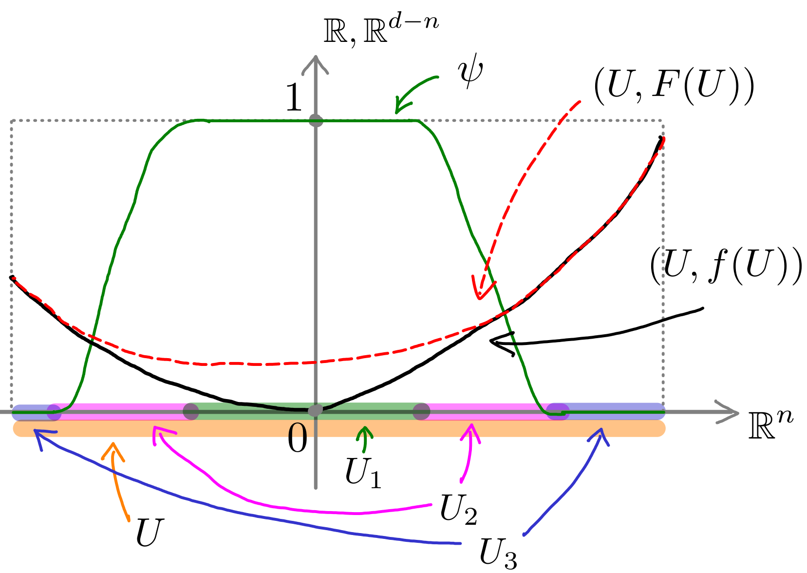
To be able to use local arguments, we need to prove that the Lipschitz constants of and its first derivative are close to the Lipschitz constants of and its first derivative.
The Lipschitz constants of the function were studied in [9], leading to a result similar to our Lemma 17. Our key contribution lies in determining the Lipschitz constant of the derivative of , a significantly more intricate task and one that is crucial for proving the main result.
Throughout the rest of this paper, we operate under the following settings:
-
We consider a function whose graph is (locally) the manifold . Such a map exists due to Theorem 27 of the full version of this article. Moreover, both and its derivative are Lipschitz, and we denote their Lipschitz constants by and , respectively.
-
We cover the domain with two sets and consider a partition of unity subordinate to this cover. We denote the partition of unity function corresponding to the set by , and the closure of its support by
We assume to be compact. We denote the Lipschitz constants of and its derivative by and , respectively, write
(3) and note that
(4) -
The (locally) smoothed manifold is then locally described by the graph of the function
(8)
Lemma 17.
The function is Lipschitz on with Lipschitz constant .
Lemma 18.
The first derivative of the function is Lipschitz on with Lipschitz constant .
3.3 On bounding the reach of in terms of Lipschitz constants
Let denote the manifold that
-
equals the graph of the function inside the neighbourhood of the point ;
-
equals outside of this neighbourhood.
Our next goal is to bound the reach of . To this end, we use a result by Federer [20] that characterizes the reach of a manifold through the distance from a point on it to a tangent space of another point on it. We provide two different bounds on this distance. In order to prove the latter, we also establish bounds on the angle between tangent spaces of the graphs of and .

We adapt the following settings, in addition to the ones established in Section 3.2: We fix two points , and label their graphs by
We write and for the graph of and , respectively, and and (resp. and ) for the tangent and affine tangent space of at (resp. of at ).
We illustrate this setup in Figure 11.
Lemma 19.
The distance between the point and the affine tangent space is bounded by
| (9) |
This has the following consequence: Let be small enough that the -neighbourhood of is contained in , . Then the graph of the function in this neighbourhood is contained in the union of balls
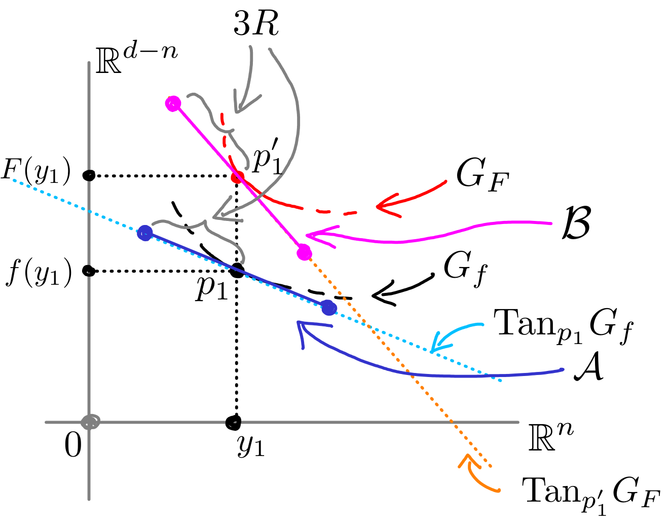
As an auxiliary result needed to prove Proposition 22, we obtain a bound on the angle between the affine tangent spaces and , as well as a bound on the Hausdorff distance between two neighbourhoods contained in these spaces. We note that the angle between two affine spaces is equal to the angle between the corresponding vector spaces. The angle between two vector subspaces and is defined as
Lemma 20.
Assume that . Then the angle between the affine tangent spaces and is bounded by
Corollary 21.
Let denote the reach of the manifold , and consider the -dimensional neighbourhood of size of the point in the affine tangent space :
Similarly, consider a -neighbourhood of the point in the affine tangent space :
Assume that . Then the Hausdorff distance between the two neighbourhoods is upper bounded:
At last, we bound the distance between the affine tangent space and a point that does not lie on the graph of . We illustrate the settings in Figure 14.
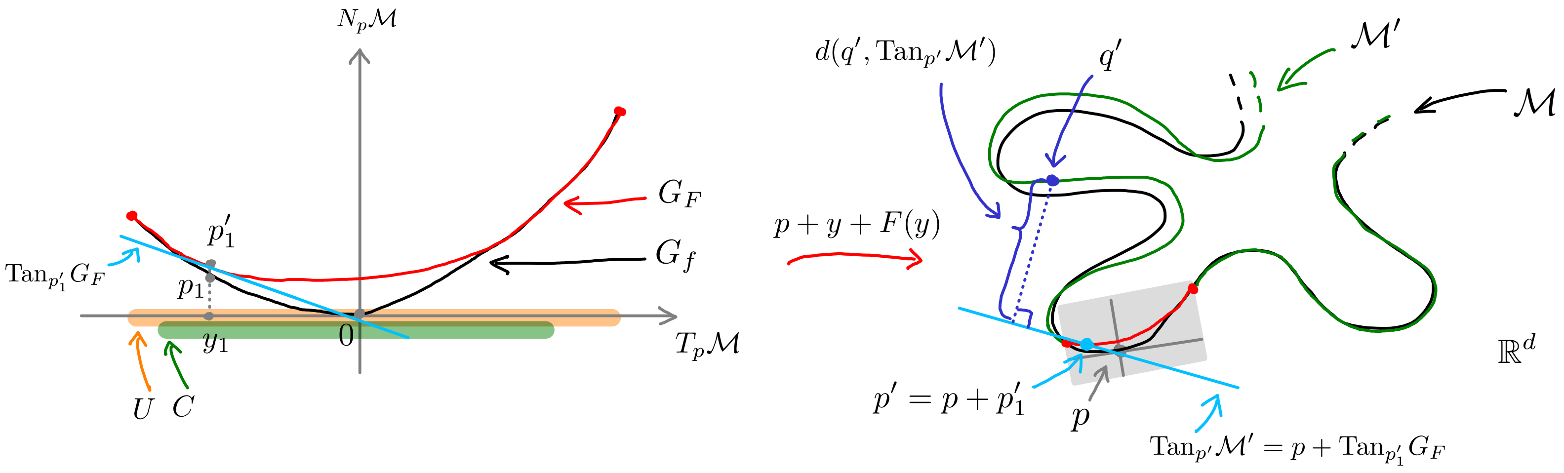
Proposition 22.
Let , and assume that . Write . Then the distance between the point and the affine tangent space is bounded by
| (10) |
Therefore, if and , then
with
4 Proof of the main theorem
We now have all the necessary tools to prove our main result. Before proceeding, let us restate the theorem: See 1
Proof.
We proceed as discussed in the introduction.
Step 1.
In the first step we select a sample of the manifold (see also Figure 15, right). To this end, we choose a parameter , and let be a -net444The factor in is almost certainly suboptimal. However, it simplifies the proof by a margin. on , meaning that
-
for every point one can find a point , such that ,
-
for all , .
Such a net exists thanks to [13, Lemma 5.2, Section 5.1.1].
Due to these properties, the -balls centred at the points of the sample cover . In addition, we consider balls of radius centred at the points of .
We need one more ingredient before we start iteratively visiting neighbourhoods of each point – a fixed partition of unity function, which we rescale at every iteration. To this end, we split the ball into three sets,
The two sets then cover the ball , and we let be the partition of unity function corresponding to the set . Then on , and on .
Next, we select a point , and restrict our attention to the ball of radius centred at .
Step 2.
Let be a function whose graph describes the manifold in the ball . To be more concrete, choose as in Theorem 27 in the full version of this article, or [26] which gives a more extensive version of Theorem 27. Due to this theorem and our choice of , the derivative of is -Lipschitz on the whole domain .

We apply the smoothing construction described in Section 3.2. As ingredients, we need a partition of unity function, and a smoothing kernel.
Partition of unity function: We map the neighbourhood diffeomorphically to the ball using the canonical identification of the tangent space with and the map . The preimages of the sets , and under this map are, respectively,
The sets and are illustrated in Figure 15, on the left. We define by scaling the partition of unity function : . Then is the partition of unity function corresponding to the set in the cover of , and thereby, on , and on . Furthermore:
Lemma 23.
The Lipschitz constants of and its derivative are bounded by and .
Step 3.
We write for the manifold that coincides with outside of the ball of radius centred at the point , and is the graph of inside this ball.
To be more concrete, we recall that we can write each point as , with . With this in mind we define, for each :
and let .
We stress that
-
inside the ball , is smooth (), and
-
not only outside of the ball , but already outside of the ball .
Next, we set forth to bound the reach of . We choose two points , and estimate the distance between and the affine tangent space – our bounds from Lemma 19 and Proposition 22 yield:
Lemma 24.
Let be two points in the manifold . Then the distance between and the affine tangent space is bounded by
with
| (12) |
Step 4.
Here we apply the smoothing construction iteratively for all points of . The correctness of the construction relies on two observations: The first observation is that (12) can be made as close to as needed. The second observation is that the manifold is locally changed only a finite number of times that (which in the non-compact case requires specific choices of , , and ).
Because is a -net, it is locally finite. In particular, the number of points of contained in a ball of radius centred at any point is , as can be seen by a simple packing argument, see e.g. [13, Lemma 5.3, Section 5.1.1] for similar arguments. However, with every iteration of the construction, the points in a neighbourhood of the point (which is the centre of the local smoothing operation) move555This size bound is not tight, in fact it can easily be improved to by noting that the part of whose projection onto falls outside is not perturbed. by at most , due to (5).
This means that the points can move at most by , where is the maximal number of times any point is visited. We claim that
Claim 25.
If we pick and assume that , then .
Proof of Claim 25.
Write for the maximal number of times any point is visited after iterations of the surgery process. The number is upper bounded by the number of points of that, during the iterative process (up to iteration ), end up in a ball of radius around the displaced point, which can move as well. Because the points move by at most and need to enter the ball of radius , they must initially lie inside a ball of radius . In other words, in order for a surgery centered at point to impact point , the original positions of and must lie at distance at most apart. Because the points in the sample are originally separated, a packing argument gives the following relation:
| (13) |
If we take sufficiently small, for example , then equation (13) is not satisfied for with . This means that for any , we have that . In particular at the end of the process the maximal number of times any point is visited is upper bounded by , i.e. .
For the given , we now choose and such that from equation (12) satisfies . This is always possible. One can set ; the choice for is a bit more subtle but choosing works if (and equivalently ) is sufficiently small. Additionally, as we have seen, has to be sufficiently small so that . This in particular means that even after the iterative process (that moves the points of ) the resulting set is still a cover, which means that every point in the manifold is smoothed. This is the reason we started with a -net and is of size .
Let be arbitrary. We now note that:
-
Every pair of points and in the manifold is visited/perturbed by the smoothing process at most times (each).
-
We have picked and such that , where here the difference between the reach and is interpreted as between each iteration of the smoothing process.
This means that the characterization of the reach (for the points and ) of Lemma 24 only changes times, and thus for a total of less than . Because the choice of and is arbitrary, the reach after the smoothing has decreased by at most .
References
- [1] Eddie Aamari, Clément Berenfeld, and Clément Levrard. Optimal reach estimation and metric learning. The Annals of Statistics, 51(3):1086–1108, 2023. doi:10.1214/23-AOS2281.
- [2] Eddie Aamari, Jisu Kim, Frédéric Chazal, Bertrand Michel, Alessandro Rinaldo, and Larry Wasserman. Estimating the reach of a manifold. Electronic journal of statistics, 13(1):1359–1399, 2019. doi:10.1214/19-EJS1551.
- [3] Eddie Aamari and Clément Levrard. Stability and minimax optimality of tangential Delaunay complexes for manifold reconstruction. Discrete & Computational Geometry, 59(4):923–971, 2018. doi:10.1007/s00454-017-9962-z.
- [4] Eddie Aamari and Clément Levrard. Nonasymptotic rates for manifold, tangent space and curvature estimation. The Annals of Statistics, 47(1), February 2019. doi:10.1214/18-aos1685.
- [5] Yariv Aizenbud and Barak Sober. Estimation of local geometric structure on manifolds from noisy data. Journal of Machine Learning Research, 26(64):1–89, 2025. URL: http://jmlr.org/papers/v26/25-0183.html.
- [6] Nina Amenta and Marshall Bern. Surface reconstruction by Voronoi filtering. In Proceedings of the Fourteenth Annual Symposium on Computational Geometry, SoCG ’98, pages 39–48, New York, NY, USA, 1998. Association for Computing Machinery. doi:10.1145/276884.276889.
- [7] Nina Amenta and Marshall Bern. Surface reconstruction by Voronoi filtering. Discrete & Computational Geometry, 22(4):481–504, December 1999. doi:10.1007/PL00009475.
- [8] Nina Amenta, Marshall Bern, and Manolis Kamvysselis. A new voronoi-based surface reconstruction algorithm. In Proceedings of the 25th Annual Conference on Computer Graphics and Interactive Techniques, SIGGRAPH ’98, pages 415–421, New York, NY, USA, 1998. Association for Computing Machinery. doi:10.1145/280814.280947.
- [9] D. Azagra, J. Ferrera, F. López-Mesas, and Y. Rangel. Smooth approximation of Lipschitz functions on Riemannian manifolds. Journal of Mathematical Analysis and Applications, 326(2):1370–1378, 2007. doi:10.1016/j.jmaa.2006.03.088.
- [10] Mikhail Belkin, Jian Sun, and Yusu Wang. Discrete laplace operator on meshed surfaces. In Proceedings of the Twenty-Fourth Annual Symposium on Computational Geometry, SCG ’08, pages 278–287, New York, NY, USA, 2008. Association for Computing Machinery. doi:10.1145/1377676.1377725.
- [11] Clément Berenfeld, John Harvey, Marc Hoffmann, and Krishnan Shankar. Estimating the reach of a manifold via its convexity defect function. Discrete & Computational Geometry, 67(2):403–438, June 2021. doi:10.1007/s00454-021-00290-8.
- [12] Harry Blum. A transformation for extracting new descriptors of shape, volume 4. MIT press Cambridge, 1967.
- [13] Jean-Daniel Boissonnat, Frédéric Chazal, and Mariette Yvinec. Geometric and Topological Inference. Cambridge Texts in Applied Mathematics. Cambridge University Press, 2018. doi:10.1017/9781108297806.
- [14] S.-W. Cheng, T.K. Dey, and J.R. Shewchuk. Delaunay Mesh Generation. Computer and information science series. CRC Press, 2013.
- [15] T.K. Dey. Curve and Surface Reconstruction: Algorithms with Mathematical Analysis. Number 23 in Cambridge monographs on applied and computational mathematics. Cambridge University Press, 2007.
- [16] M.P. do Carmo. Differential Geometry of Curves and Surfaces. Prentice-Hall, 1976.
- [17] M.P. do Carmo. Riemannian Geometry. Birkhäuser, 1992.
- [18] Paul Erdős. Some remarks on the measurability of certain sets. Bulletin of the American Mathematical Society, 51(10):728–731, 1945.
- [19] Paul Erdős. On the Hausdorff dimension of some sets in Euclidean space. Bulletin of the American Mathematical Society, 52(2):107–109, 1946. doi:10.1090/S0002-9904-1946-08514-6.
- [20] H. Federer. Curvature measures. Transactions of the America Mathematical Society, 93:418–491, 1959.
- [21] H. Federer. Geometric Measure Theory. Classics in Mathematics. Springer, 1996.
- [22] Charles Fefferman, Sergei Ivanov, Yaroslav Kurylev, Matti Lassas, and Hariharan Narayanan. Reconstruction and interpolation of manifolds. I: The geometric Whitney problem. Foundations of Computational Mathematics, 2019. doi:10.1007/s10208-019-09439-7.
- [23] Charles Fefferman, Sergei Ivanov, Matti Lassas, and Hariharan Narayanan. Fitting a manifold of large reach to noisy data. Journal of Topology and Analysis, 17(02):315–396, July 2023. doi:10.1142/s1793525323500012.
- [24] M.W. Hirsch. Differential Topology. Springer-Verlag: New York, Heidelberg, Berlin, 1976.
- [25] Norbert Kleinjohann. Nächste Punkte in der Riemannschen Geometrie. Mathematische Zeitschrift, 176(3):327–344, 1981. doi:10.1007/BF01214610.
- [26] André Lieutier and Mathijs Wintraecken. Manifolds of positive reach, differentiability, tangent variation, and attaining the reach. In Hee-Kap Ahn, Michael Hoffmann, and Amir Nayyeri, editors, 42nd International Symposium on Computational Geometry (SoCG 2026), volume 367 of Leibniz International Proceedings in Informatics (LIPIcs), pages 74:1–74:16, Dagstuhl, Germany, 2026. Schloss Dagstuhl – Leibniz-Zentrum für Informatik. doi:10.4230/LIPIcs.SoCG.2026.74.
- [27] Alexander Lytchak. On the geometry of subsets of positive reach. manuscripta mathematica, 115(2):199–205, 2004. doi:10.1007/s00229-004-0491-8.
- [28] Alexander Lytchak. Almost convex subsets. Geometriae Dedicata, 115(1):201–218, 2005. doi:10.1007/s10711-005-5994-2.
- [29] Marina Meilă and Hanyu Zhang. Manifold learning: What, how, and why. Annual Review of Statistics and Its Application, 11(1):393–417, April 2024. doi:10.1146/annurev-statistics-040522-115238.
- [30] David Milman and Zeev Waksman. On topological properties of the central set of a bounded domain in . Journal of Geometry, 15(1):1–7, 1980. doi:10.1007/BF01919351.
- [31] Sumner Byron Myers. Connections between differential geometry and topology I Simply connected surfaces. Duke Math. J., 1(1):376–391, 1935.
- [32] Sumner Byron Myers. Connections between differential geometry and topology II Closed surfaces. Duke Math. J., 2(1):95–102, 1936.
- [33] P. Niyogi, S. Smale, and S. Weinberger. Finding the homology of submanifolds with high confidence from random samples. Discrete & Computational Geometry, 39(1-3):419–441, 2008. doi:10.1007/s00454-008-9053-2.
- [34] Henri Poincaré. Sur les lignes géodésiques des surfaces convexes. Transactions of the American Mathematical Society, 6(3):237–274, 1905.
- [35] Ludovic Rifford. From the poincaré “lignes de partage” to the convex earth theorem. https://math.univ-cotedazur.fr/˜rifford/Papiers_en_ligne/IHP100_Talk_LR.pdf.
- [36] Barak Sober and David Levin. Manifold approximation by moving least-squares projection (MMLS). Constructive Approximation, pages 1–46, 2019. doi:10.1007/s00365-019-09489-8.
- [37] Yuan Wang and Bei Wang. Topological inference of manifolds with boundary. Computational Geometry, 88:101606, 2020. doi:10.1016/j.comgeo.2019.101606.
- [38] John Henry Constantine Whitehead. On the covering of a complete space by the geodesics through a point. Annals of Mathematics, 36(3):679–704, 1935.