Locality Sensitive Hashing in Hyperbolic Space

Locality Sensitive Hashing (LSH) is a hashing scheme in which similar items are more likely to hash to the same bucket. Indyk and Motwani, in their seminal work [27, 25], developed LSH for general metric spaces and provided hash function constructions for the Hamming distance. The LSH framework provides an efficient data structure for the Approximate Nearest Neighbor Search (ANNS) problem, which is particularly challenging in the high-dimensional regimes. Since then, LSH has been developed for various similarity measures such as ${\mathrm{\ell }}_1$ [1, 35], ${\mathrm{\ell }}_2$ [18, 2], ${\mathrm{\ell }}_p$ [18], cosine similarity [15], Jaccard similarity [11, 10], angular (spherical) distances [47], etc. With support for similarity search, data independence, mild dependence on data dimension, and simplicity in implementation, LSH serves as an algorithmic tool for classical problems such as clustering, near-duplicate detection, and efficient information retrieval for very large datasets. LSH has also been used widely in database and machine learning pipelines in industry [22, 12, 16, 44, 42, 17, 32, 4, 7]. For a nice survey, please refer to [2].

Hyperbolic geometry is a non-Euclidean geometry. It drops the parallel postulate of Euclidean geometry. In hyperbolic geometry, for any line and a point not on that line, there are at least two distinct lines through the point that do not intersect the original line. Hyperbolic geometry has received increasing attention in modern data analysis because it naturally models hierarchical, tree-like, and exponentially branching structures that arise throughout science and technology. Unlike Euclidean spaces, where volume grows polynomially, hyperbolic spaces exhibit exponential volume growth, matching the combinatorial growth of hierarchies, taxonomies, knowledge graphs, and high-dimensional networks with latent tree-like structure. This geometric compatibility yields embeddings with dramatically reduced distortion: objects that are far apart in a hierarchy can be faithfully separated, and geodesics efficiently capture ancestry, flow, and community structure. As a result, hyperbolic embeddings now underpin state-of-the-art methods in network representation learning, hierarchical clustering, and discrete geometric data analysis [38, 24, 21, 48, 19, 13, 14, 49, 30, 46]. It is also the most important space representing the negative curvature phenomena arising from complex geometric situations [34, 45]. Namely, according to Gromov’s hyperbolization program [23], spaces with complicated topology tend to resemble spaces with negative curvature. Hyperbolic geometry provides the fundamental model for negatively curved spaces, offering the canonical framework in which their curvature and geometric behavior are understood.

Moreover, the hyperbolic plane offers an unusually tractable analytic structure: its constant negative curvature provides explicit formulas for distance, geodesics, convexity, and isometries, enabling efficient optimization for machine-learning tasks. Its rich isometry group and uniformization properties are directly linked to complex analysis and conformal representations, providing tools that scale from theoretical guarantees to practical algorithms for dimensionality reduction, visualization, and manifold learning.

These applications provide strong motivation for developing efficient algorithms in hyperbolic space, and in this paper, we study locality-sensitive hashing in hyperbolic space, a topic that, to our best knowledge, has not been studied before.

In this section, we show the LSH construction in ${ℍ}^2$ that yields Theorem 4. We adopt the Poincaré disk model for points in ${ℍ}^2$, defined on the unit disk . The space is equipped with the metric $ds=\frac{2|dz|}{1-{|z|}^2}$, which induces the following distance function:

Geometrically, geodesics in $𝔻$ correspond to circular arcs orthogonal to the unit circle boundary $C_{\mathrm{\infty }}$, with diameters passing through the origin as special cases.

The locality sensitive hash functions we use are random geodesics in the Poincaré disk model. For this purpose we require a well-defined probability measure on the set of all geodesics to ensure that random sampling of geodesics is meaningful and invariant under hyperbolic isometries. Luckily, the classical integral geometry [43] provides the needed theory. Integral geometry studies the measures on the spaces of all lines, or totally geodesic planes in Euclidean, hyperbolic, or spherical spaces, such that the measures are invariant under isometries. The fundamental theorems of Poincaré, Cauchy and Crofton show that one can recover basic geometric quantities such as lengths, areas, or volumes of an object by averaging over the set of geodesics intersecting the object.

In the hyperbolic plane, the isometrically invariant probability measure on the space of all geodesics is given by the kinematic measure [43]. Take a point $q$ and a non-zero tangent vector $v$ at $q$ in the hyperbolic plane. The polar coordinate of a geodesic $\gamma$ with respect to $(q,v)$ is a pair $(t,\theta )$ where $t$ is the hyperbolic distance from $\gamma$ to $q$ and $\theta$ is the angle of the perpendicular from $q$ to $\gamma$ with the tangent vector $v$. The kinematic measure in geodesic polar coordinates $(t,\theta )$ is

The remarkable feature of the above formula is that it is independent of the choices of $q$ and $v$. This measure reflects the fact that the volume element in hyperbolic geometry grows exponentially with $t$.

Since the space of all geodesics in ${ℍ}^2$ has infinite total measure, we limit our choices of geodesics in the family of all geodesics intersecting a hyperbolic disk $B(0,R)$ of radius $R$ centered at the origin. By Crofton’s formula, the measure of the set of geodesics that intersect a convex body is proportional to the perimeter of that body. Specifically, the corresponding measure is obtained by integrating the invariant element $d\mu$ over the disk:

Now, we choose $R$ such that the disk $B(0,R)$ centered at the origin with radius $R$ contains all points of $P$. Our final bound on the performance parameter $\rho$ does not depend on $R$, and in practice, one can choose $R$ to be a sufficiently large value. Note that in practice, hyperbolic embedding typically avoids using points that are far from the origin due to practical concerns on resolution and numerical instability [36].

A geodesic $\gamma$ is chosen with probability density function $\frac{\cosh (t)}{2\pi \sinh (R)}$ to be at polar coordinate $(t,\theta )$ where $t$ is taken from $[0,R]$ and $\theta$ is taken from $[0,2\pi )$. In the Poincaré disk model, geodesics appear as Euclidean circular arcs, so $\gamma$ is a circular arc with Euclidean center $c\in {ℝ}^2$ and radius $b>0$. Specifically, define $c=\coth (t)e^{i\theta }$ (here convert $e^{i\theta }$ from the complex plane to the Euclidean plane) and $b=1/\sinh t$. Define a hash function ${ℍ}^2\to \{-1,1\}$ by

where $x$ is the Euclidean coordinate of a point in ${ℍ}^2$. We can also rewrite the geodesic $\gamma$ using the Minkowski model with inner product $⟨z,z⟩=-z_1^2+z_2^2+z_3^2$. Let the geodesic $\gamma$ be given by $\{x\in {ℍ}^2|⟨x,u⟩=0\}$ for a point $u$ in the de Sitter space $\{y\in {ℝ}^{2,1}|⟨y,y⟩=1\}$:

Note that $(t,\theta )$ is polar coordinate with respect to the point $q=(1,0,0)$ and $v=(0,1,0)$. Then the formula for $h_{\gamma }(x)$ is $\text{sgn}⟨x,u⟩.$ This is exactly the same formula as in the Euclidean space. The advantage of this formula over the above one is that it is intrinsic to hyperbolic geometry, i.e., invariant under hyperbolic isometry.

With this setup, we present the hash function in ${ℍ}^2$ below.

For brevity, we write $h(x)$ for $h_{\gamma }(x)$ when it is clear from context. Figure 1 demonstrates how the hash function works as a separator.

The key to proving Theorem 4 is a characterization of the collision probability under our hashing scheme, given in the following lemma.

In this section, we prove the dimension reduction result (Theorem 12). We use the Poincaré half-space model of the hyperbolic space ${ℍ}^d$. Each point in ${ℍ}^d$ is represented by a pair $(z,x)$ with $z\in {ℝ}^{+}$ and $x\in {ℝ}^{d-1}$. The hyperbolic distance between two points $p_1=(z_1,x_1)$ and $p_2=(z_2,x_2)$ is defined by the following function

where $\Vert x_1-x_2\Vert$ is the Euclidean distance between $x_1,x_2$. For a set of $n$ points $P=\{p_i=(z_i,x_i)\}\subseteq {ℍ}^d$, we would like to perform dimension reduction to generate $P^{\prime }=\{p_i^{\prime }\}$ in ${ℍ}^k$ and keep the pairwise distances similar. The method by Benjamini and Makarychev [9] is to perform dimension reduction for the Euclidean point set $X=\{x_i\}\subseteq {ℝ}^{d-1}$ by a function $f$ to $X^{\prime }=\{x_i^{\prime }\}\subseteq {ℝ}^{k-1}$ and define $P^{\prime }=\{p_i^{\prime }\}$ with $p_i^{\prime }=(z_i,x_i^{\prime })$ in ${ℍ}^k$. Below, we present a refined analysis that yields slightly tighter bounds on the distortion. Essentially, we show that the bound on the distortion of the Euclidean distances of $X^{\prime }$ (compared to $X$) carries over to bound the distortion of the hyperbolic distance of $P^{\prime }$ compared to $P$.

The proof follows the main idea in [9], but we have slightly improved analysis and bounds. Specifically, the main idea is to analyze the behavior of the function

which is an increasing function of $r$, when $z_1,z_2>0$. For completeness, we include the full proof in the full version [20].

A distribution $D$ is called $p$-stable [51] with $p\ge 0$ if for any $n$ real numbers $v_1,v_2,\mathrm{\cdots },v_n$ and random independent variables $X_1,X_2,\mathrm{\cdots }{X}_n$ with distribution $D$, ${\sum }_i{v}_i{X}_i$ has the same distribution as the variable ${({\sum }_i{|v_i|}^p)}^{1/p}X$, where $X$ is a random variable with distribution $D$. A Gaussian distribution $𝒩(0,1)$ is $2$-stable. This property has been used to build Euclidean LSH [18], to sketch high-dimensional vectors [26], and for many other applications.

Consider $n$ points $P=\{p_i\}$ in ${ℍ}^d$. We use random projection to project these points to $P^{\prime }=\{p_i^{\prime }\}$ in ${ℍ}^2$ using the method in Section 3. In particular, we take a vector $\overrightarrow{a}$ with dimension $d-1$ where each entry is independently taken from a Gaussian distribution $𝒩(0,1)$. For $p_i=(z_i,x_i)$ in the upper half space model, we have $p_i=(z_i,x_i^{\prime })$ in ${ℍ}^2$, where $x_i^{\prime }=\overrightarrow{a}\cdot x_i$. We then use the LSH mechanism in Section 2 to map these points into buckets. In this section, we analyze the performance of this mechanism.

In our case, the value $\overrightarrow{a}\cdot (p-q)$ for any two vectors $p,q\in {ℝ}^{d-1}$ is also a Gaussian distribution with zero mean and variance ${\Vert p-q\Vert }^2$, or, the distribution of $\Vert p-q\Vert Z$ with $Z\sim 𝒩(0,1)$. Take $f(z)$ to be the probability density function of the absolute value of $𝒩(0,1)$:

To calculate the probability that $p_1,p_2$ are mapped to the same bucket, we take $s=\Vert x_1-x_2\Vert$ and $r=d_{ℍ}(p_1,p_2)=F_{z_1,z_2}(s)$, where

is an increasing function of $s$. Suppose $p_1,p_2$ are mapped to points $p_1^{\prime },p_2^{\prime }$ with $s^{\prime }=\Vert x_1^{\prime }-x_2^{\prime }\Vert$ and $r^{\prime }=d_{ℍ}(p_1^{\prime },p_2^{\prime })=F_{z_1,z_2}(s^{\prime })$. $s^{\prime }$ follows the distribution of $sZ$ with $Z\sim 𝒩(0,1)$. Recall that using the LSH for ${ℍ}^2$ the probability that $p_1^{\prime },p_2^{\prime }$ map to the same bucket is $1-\frac{r^{\prime }}{w}$ where $w=2\sinh R$. Now we have,

We can get an upper bound of $p(r)$.

The lower bound on the performance parameter $\rho$ for LSH of ${\mathrm{\ell }}_p$ metrics has been studied in [37, 40]. Theorem 5.2 in [40] stated that for points of the Hamming cube ${\{0,1\}}^d$ and some , an $(r,R,p_1,p_2)$-sensitive LSH of Hamming distance, with $r=\delta d/c$ and $R=\delta d$, must have

This lower bound can be used to generate a lower bound of $1/c^p$ for ${\mathrm{\ell }}_p$ distance – by using ${\mathrm{\ell }}_p$ distance on the same point set. In particular, it shows that LSH for Euclidean distances has $\rho \ge 1/c^2$. We will use the same construction to show a lower bound on $\rho$ for hyperbolic distance.

We implement our Locality Sensitive Hashing algorithms in both ${ℍ}^2$ and ${ℍ}^d$. We aim to evaluate the LSH performance in terms of $\rho$ in practice.

We first explain the synthetic data we use. For each $d\in \{2,10,100,1000\}$, we generate a dataset of 1000 points by uniformly random sampling in a hyperbolic sphere of the same radius, $R=\log (199)$. This radius was chosen so that after the points are projected to ${ℍ}^2$ and mapped to the Poincare disk model, the points lie inside a Euclidean circle of radius 0.99. Further, we set $r=0.2$ with varying $c=1.5+k$ for $k=0,1\mathrm{\dots }17$ to compute the value of $p_1$ and $p_2$. We illustrate results on $p_1,p_2$ in Figure 3 and $\rho$ in Figure 4 for different choices of $c$ obtained by averaging over 1000 repetitions.

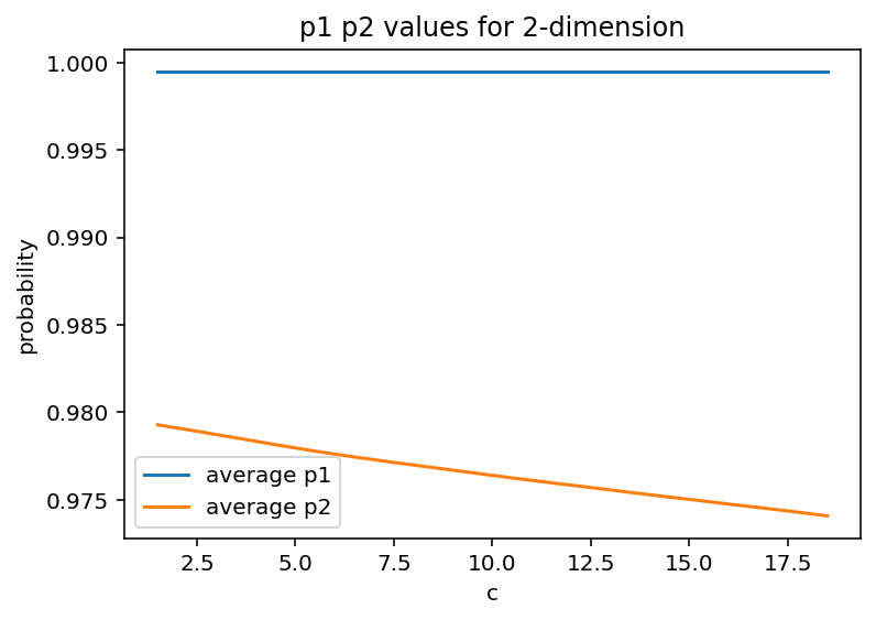
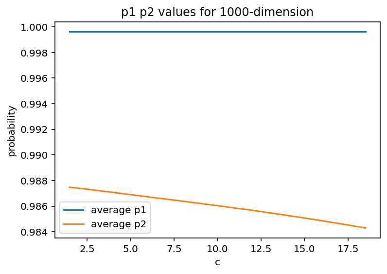
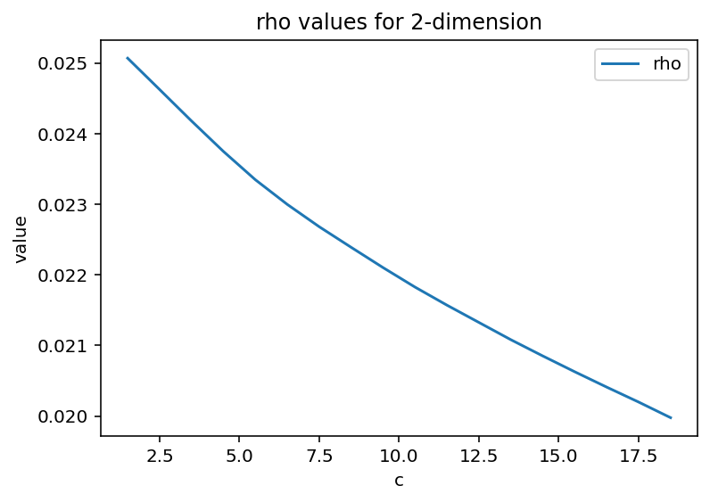
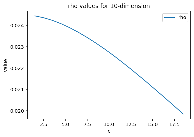
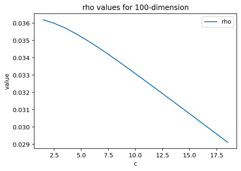
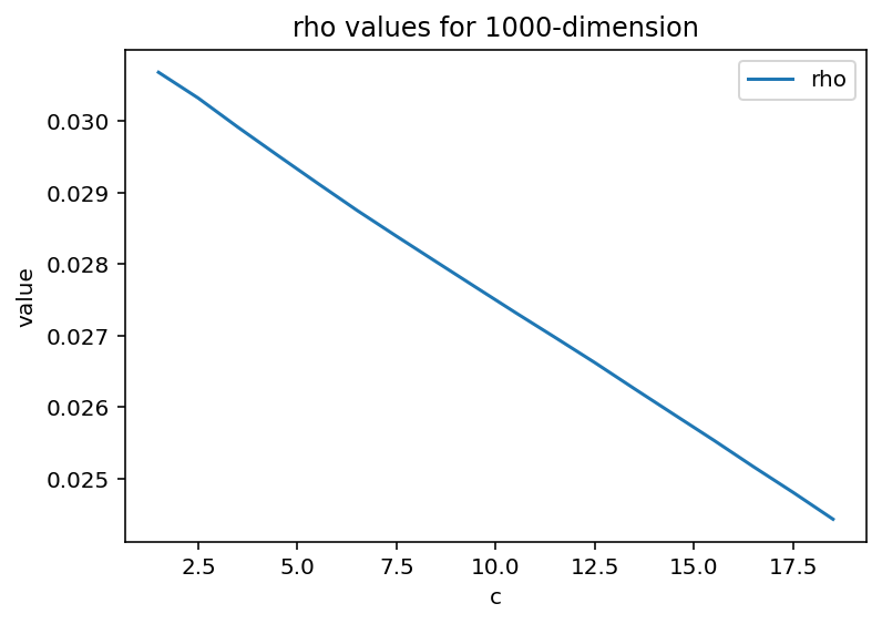
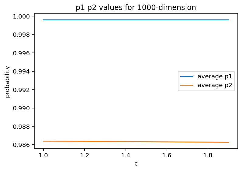
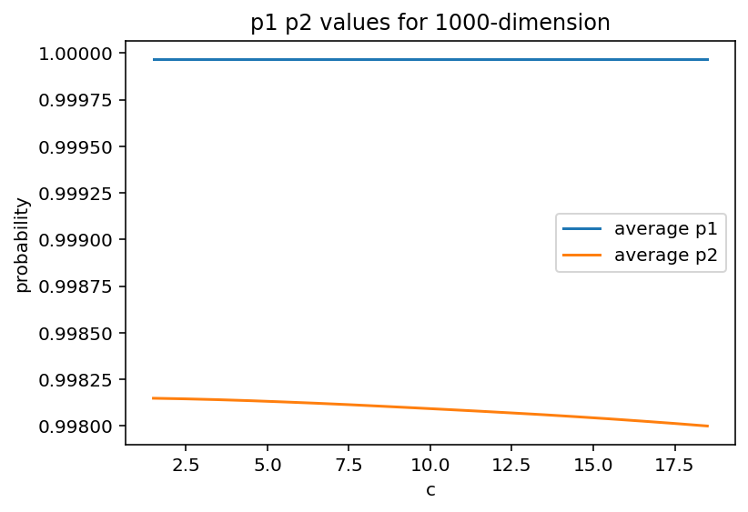
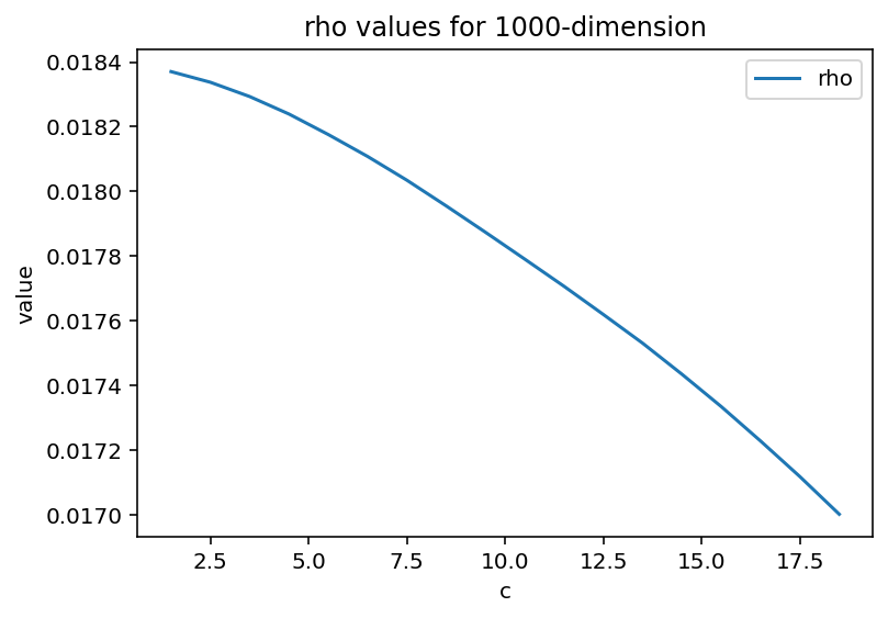
We see that, as expected, $p_1$ and $p_2$ are close to 1 in all cases. Due to the randomness of the data, the probabilities vary slightly in percentage. Since $\rho$ is related to the complements of these probabilities, varying slightly in proportion when so close to 1 causes the significant differences in $\rho$ values that we are observing. However, in all cases, the $\rho$ graphs are below $1/c$. We note that they are not exactly $1/c$ because we considered all pairs of points with distance below $r$ or above $cr$, not exactly equal to $r$ or $cr$, so $1/c$ should be an upper bound of what we obtain.

Next, we use the same data for $d=2$, but vary $c=1+.1k$ for $k=1,\mathrm{\dots }10$ to see if the LSH still works for small values of $c$ even though our proof only has guarantees for $c\ge 1.59$. From Figure 5 we see fairly similar results, just $p_2$ varying less, but LSH still achieves $\rho$ lower than $\frac{1}{c}$.

We also generated some data for $d=1000$, varying $R$ so that the points lie in a circle of Euclidean radii $.9$ and $.999$. We see that $p_1,p_2$ and $\rho$ change a little, but not significantly and still fall well within the theoretical bounds.

Lastly, we generate similar data for $d=2$, but containing 2000 points. Then, we analyze $p_1$ and $p_2$ for pairs of points that are at the boundary of acceptable distances. Precisely, we choose pairs of points that have distance within $[.9r,r]$ or $[cr,1.1cr]$. This gives us an approximately linear graph for $p_2$ and $\rho$ curve that approximates $\frac{1}{c}$.

The experiment setup with a fixed $r$ and a reasonably large constant $c$ (rather than $1+\epsilon$ for a very small $\epsilon$) is motivated by real world applications such as similarity learning which focuses on differentiating data elements that are very similar or sufficiently far away. Many data modalities and data tasks fall into this category. For example, in image recognition the goal is to recognize two pictures with similar scenes or semantics. But for two pictures on completely different subjects, it is sufficient to know that they are far away and the exact values of dissimilarities are less important. One important take-away message from our experiments is that the empirical value of $\rho$ with the synthetic data set is very small with a mild dependency on dimension and decreasing value of $c$. It is much smaller than our theoretical upper bound – partly because we consider all pairs whose distance are often much smaller than $r$ or much greater than $cr$. Since the storage requirement for approximate nearest neighbor data structure built with LSH grows in terms of $O(n^{1+\rho })$ and the query cost grows in terms of $O(n^{\rho })$. The empirical small value of $\rho$ suggests great potential for practical use.

References

- [1] Alexandr Andoni and Piotr Indyk. Efficient algorithms for substring near neighbor problem. In Proceedings of the seventeenth annual ACM-SIAM symposium on Discrete algorithm - SODA ’06, pages 1203–1212, New York, New York, USA, 2006. ACM Press. URL: http://dl.acm.org/citation.cfm?id=1109557.1109690.
- [2] Alexandr Andoni and Piotr Indyk. Near-optimal hashing algorithms for approximate nearest neighbor in high dimensions. Communications of the ACM, 51(1):117–122, 2008. doi:10.1145/1327452.1327494.
- [3] Alexandr Andoni, Piotr Indyk, Thijs Laarhoven, Ilya Razenshteyn, and Ludwig Schmidt. Practical and optimal LSH for angular distance. In C. Cortes, N. Lawrence, D. Lee, M. Sugiyama, and R. Garnett, editors, Advances in Neural Information Processing Systems, volume 28, pages 1225–1233. Curran Associates, Inc., 2015. URL: https://proceedings.neurips.cc/paper_files/paper/2015/file/2823f4797102ce1a1aec05359cc16dd9-Paper.pdf.
- [4] Alexandr Andoni, Piotr Indyk, Huy L Nguyen, and Ilya Razenshteyn. Beyond locality-sensitive hashing. In Proceedings of the Twenty-Fifth Annual ACM-SIAM Symposium on Discrete Algorithms, pages 1018–1028. Society for Industrial and Applied Mathematics, Philadelphia, PA, January 2014.
- [5] Alexandr Andoni, Assaf Naor, Aleksandar Nikolov, Ilya Razenshteyn, and Erik Waingarten. Data-dependent hashing via nonlinear spectral gaps. In Proceedings of the 50th annual ACM SIGACT symposium on theory of computing, pages 787–800, 2018. doi:10.1145/3188745.3188846.
- [6] Alexandr Andoni, Assaf Naor, Aleksandar Nikolov, Ilya Razenshteyn, and Erik Waingarten. Hölder homeomorphisms and approximate nearest neighbors. In 2018 IEEE 59th Annual Symposium on Foundations of Computer Science (FOCS), pages 159–169. IEEE, 2018. doi:10.1109/FOCS.2018.00024.
- [7] Alexandr Andoni and Ilya Razenshteyn. Optimal data-dependent hashing for approximate near neighbors. In Proceedings of the forty-seventh annual ACM symposium on Theory of Computing, pages 793–801, New York, NY, USA, June 2015. ACM. doi:10.1145/2746539.2746553.
- [8] Alexandr Andoni and Ilya Razensteyn. Tight Lower Bounds for Data-Dependent Locality-Sensitive Hashing. In Sándor Fekete and Anna Lubiw, editors, 32nd International Symposium on Computational Geometry (SoCG 2016), volume 51 of Leibniz International Proceedings in Informatics (LIPIcs), pages 9:1–9:11, Dagstuhl, Germany, 2016. Schloss Dagstuhl – Leibniz-Zentrum für Informatik. doi:10.4230/LIPIcs.SoCG.2016.9.
- [9] Itai Benjamini and Yury Makarychev. Dimension reduction for hyperbolic space. Proceedings of the American Mathematical Society, pages 695–698, 2009.
- [10] Andrei Z Broder. On the resemblance and containment of documents. In Proceedings. Compression and Complexity of SEQUENCES 1997 (Cat. No.97TB100171), pages 21–29. IEEE Comput. Soc, 2002.
- [11] Andrei Z Broder, Steven C Glassman, Mark S Manasse, and Geoffrey Zweig. Syntactic clustering of the web. Comput. Netw. ISDN Syst., 29(8-13):1157–1166, 1997. doi:10.1016/S0169-7552(97)00031-7.
- [12] Jeremy Buhler. Efficient large-scale sequence comparison by locality-sensitive hashing. Bioinformatics, 17(5):419–428, 2001. doi:10.1093/BIOINFORMATICS/17.5.419.
- [13] Ines Chami, Adva Wolf, Da-Cheng Juan, Frederic Sala, Sujith Ravi, and Christopher Ré. Low-dimensional hyperbolic knowledge graph embeddings. In Proceedings of the 58th Annual Meeting of the Association for Computational Linguistics, pages 6901–6914, Stroudsburg, PA, USA, 2020. Association for Computational Linguistics. doi:10.18653/V1/2020.ACL-MAIN.617.
- [14] Ines Chami, Rex Ying, Christopher Ré, and Jure Leskovec. Hyperbolic graph convolutional neural networks. Adv. Neural Inf. Process. Syst., pages 4869–4880, 2019.
- [15] Moses S Charikar. Similarity estimation techniques from rounding algorithms. In Proceedings of the thiry-fourth annual ACM symposium on Theory of computing, pages 380–388, 2002. doi:10.1145/509907.509965.
- [16] Edith Cohen, Mayur Datar, Shinji Fujiwara, Aristides Gionis, Piotr Indyk, Rajeev Motwani, Jeffrey D Ullman, and Cheng Yang. Finding interesting associations without support pruning. IEEE Transactions on Knowledge and Data Engineering, 13(1):64–78, 2002. doi:10.1109/69.908981.
- [17] Abhinandan S Das, Mayur Datar, Ashutosh Garg, and Shyam Rajaram. Google news personalization: scalable online collaborative filtering. In Proceedings of the 16th international conference on World Wide Web, pages 271–280, 2007.
- [18] Mayur Datar, Nicole Immorlica, Piotr Indyk, and Vahab S Mirrokni. Locality-sensitive hashing scheme based on -stable distributions. In Proceedings of the twentieth annual symposium on Computational geometry, pages 253–262, 2004. doi:10.1145/997817.997857.
- [19] Christopher De Sa, Albert Gu, Christopher Ré, and Frederic Sala. Representation tradeoffs for hyperbolic embeddings. Proc. Mach. Learn. Res., pages 4460–4469, 2018.
- [20] Chengyuan Deng, Jie Gao, Kevin Lu, Feng Luo, and Cheng Xin. Locality sensitive hashing in hyperbolic space, 2026. arXiv:2603.19724.
- [21] Octavian Ganea, Gary Becigneul, and Thomas Hofmann. Hyperbolic neural networks. In S. Bengio, H. Wallach, H. Larochelle, K. Grauman, N. Cesa-Bianchi, and R. Garnett, editors, Advances in Neural Information Processing Systems, volume 31, pages 5350–5360. Curran Associates, Inc., 2018. URL: https://proceedings.neurips.cc/paper_files/paper/2018/file/dbab2adc8f9d078009ee3fa810bea142-Paper.pdf.
- [22] Aristides Gionis, Piotr Indyk, and Rajeev Motwani. Similarity search in high dimensions via hashing. In Proceedings of the 25th International Conference on Very Large Data Bases, VLDB ’99, pages 518–529, San Francisco, CA, USA, 1999. Morgan Kaufmann Publishers Inc. URL: http://www.vldb.org/conf/1999/P49.pdf.
- [23] M. Gromov. Hyperbolic groups. In Essays in group theory, volume 8 of Math. Sci. Res. Inst. Publ., pages 75–263. Springer, New York, 1987. doi:10.1007/978-1-4613-9586-7_3.
- [24] Caglar Gulcehre, Misha Denil, Mateusz Malinowski, Ali Razavi, Razvan Pascanu, Karl Moritz Hermann, Peter Battaglia, Victor Bapst, David Raposo, Adam Santoro, and Nando de Freitas. Hyperbolic attention networks. In International Conference on Learning Representations, 2019. URL: https://openreview.net/forum?id=rJxHsjRqFQ.
- [25] Sariel Har-Peled, Piotr Indyk, and Rajeev Motwani. Approximate nearest neighbor: Towards removing the curse of dimensionality. Theory of Computing, 8(14):321–350, 2012. doi:10.4086/toc.2012.v008a014.
- [26] Piotr Indyk. Stable distributions, pseudorandom generators, embeddings, and data stream computation. J. ACM, pages 307–323, 2006. doi:10.1145/1147954.1147955.
- [27] Piotr Indyk and Rajeev Motwani. Approximate nearest neighbors: towards removing the curse of dimensionality. In Proceedings of the thirtieth annual ACM symposium on Theory of computing, pages 604–613, 1998. doi:10.1145/276698.276876.
- [28] Rajesh Jayaram, Erik Waingarten, and Tian Zhang. Data-dependent LSH for the earth mover’s distance. In Proceedings of the 56th Annual ACM Symposium on Theory of Computing, pages 800–811, New York, NY, USA, June 2024. ACM. doi:10.1145/3618260.3649666.
- [29] William B Johnson and Joram Lindenstrauss. Extensions of Lipschitz mappings into a Hilbert space. Contemporary mathematics, 26(189-206):1, 1984.
- [30] Baki Karlia. Edge matrix of hyperbolic simplices. Geom. Dedicata, 109(1):1–6, December 2004.
- [31] Sándor Kisfaludi-Bak and Geert van Wordragen. A Quadtree, a Steiner spanner, and approximate nearest neighbours in Hyperbolic space. In Wolfgang Mulzer and Jeff M. Phillips, editors, 40th International Symposium on Computational Geometry (SoCG 2024), volume 293 of Leibniz International Proceedings in Informatics (LIPIcs), pages 68:1–68:15, Dagstuhl, Germany, 2024. Schloss Dagstuhl – Leibniz-Zentrum für Informatik. doi:10.4230/LIPIcs.SoCG.2024.68.
- [32] Hisashi Koga, Tetsuo Ishibashi, and Toshinori Watanabe. Fast agglomerative hierarchical clustering algorithm using locality-sensitive hashing. Knowl. Inf. Syst., 12(1):25–53, May 2007. doi:10.1007/S10115-006-0027-5.
- [33] Robert Krauthgamer and James Lee. Algorithms on negatively curved spaces. In 2006 47th Annual IEEE Symposium on Foundations of Computer Science (FOCS’06), pages 119–132. IEEE, 2006. doi:10.1109/FOCS.2006.9.
- [34] Dmitri Krioukov, Fragkiskos Papadopoulos, Maksim Kitsak, Amin Vahdat, and Marián Boguñá. Hyperbolic geometry of complex networks. Physical Review E, 82(3):036106, September 2010. doi:10.1103/PhysRevE.82.036106.
- [35] Nathan Linial, Eran London, and Yuri Rabinovich. The geometry of graphs and some of its algorithmic applications. In Proceedings 35th Annual Symposium on Foundations of Computer Science, pages 577–591. IEEE Comput. Soc. Press, 2002.
- [36] Gal Mishne, Zhengchao Wan, Yusu Wang, and Sheng Yang. The numerical stability of hyperbolic representation learning. In Andreas Krause, Emma Brunskill, Kyunghyun Cho, Barbara Engelhardt, Sivan Sabato, and Jonathan Scarlett, editors, Proceedings of the 40th International Conference on Machine Learning, volume 202 of Proceedings of Machine Learning Research, pages 24925–24949. PMLR, 23–29 July 2023. URL: https://proceedings.mlr.press/v202/mishne23a.html.
- [37] Rajeev Motwani, Assaf Naor, and Rina Panigrahi. Lower bounds on locality sensitive hashing. In Proceedings of the twenty-second annual symposium on Computational geometry, pages 154–157, 2006. doi:10.1145/1137856.1137881.
- [38] Maximilian Nickel and Douwe Kiela. Poincaré embeddings for learning hierarchical representations. In Proceedings of the 31st International Conference on Neural Information Processing Systems, NIPS’17, pages 6341–6350, Red Hook, NY, USA, 2017. Curran Associates Inc.
- [39] Frank Nielsen and Richard Nock. Hyperbolic voronoi diagrams made easy. In 2010 International Conference on Computational Science and Its Applications. IEEE, 2010.
- [40] Ryan O’Donnell, Yi Wu, and Yuan Zhou. Optimal lower bounds for locality-sensitive hashing (except when is tiny). ACM Transactions on Computation Theory (TOCT), 6(1):1–13, 2014. doi:10.1145/2578221.
- [41] Liudmila Prokhorenkova, Dmitry Baranchuk, Nikolay Bogachev, Yury Demidovich, and Alexander Kolpakov. Graph-based nearest neighbor search in hyperbolic spaces. In International Conference on Learning Representations, 2022. URL: https://openreview.net/forum?id=USIgIY6TNDe.
- [42] Deepak Ravichandran, Patrick Pantel, and Eduard Hovy. Randomized algorithms and NLP: Using locality sensitive hash functions for high speed noun clustering. In Proceedings of the 43rd Annual Meeting of the Association for Computational Linguistics (ACL’05), pages 622–629, 2005. doi:10.3115/1219840.1219917.
- [43] Luis A Santalo and Mark Kac. Integral geometry and geometric probability. Cambridge University Press, Cambridge, October 2004.
- [44] Shakhnarovich, Viola, and Darrell. Fast pose estimation with parameter-sensitive hashing. In Proceedings Ninth IEEE International Conference on Computer Vision, pages 750–757. IEEE, 2003.
- [45] Yuval Shavitt and Tomer Tankel. On the curvature of the Internet and its usage for overlay construction and distance estimation. In IEEE INFOCOM 2004, volume 1, page 384. IEEE, 2004. doi:10.1109/INFCOM.2004.1354510.
- [46] Puoya Tabaghi, Michael Khanzadeh, Yusu Wang, and Siavash Mirarab. Principal component analysis in space forms. IEEE Trans. Signal Process., 72:4428–4443, 2024. doi:10.1109/TSP.2024.3457529.
- [47] Kengo Terasawa and Yuzuru Tanaka. Spherical LSH for approximate nearest neighbor search on unit hypersphere. In Lecture Notes in Computer Science, Lecture notes in computer science, pages 27–38. Springer Berlin Heidelberg, Berlin, Heidelberg, 2007. doi:10.1007/978-3-540-73951-7_4.
- [48] Alexandru Tifrea, Gary Becigneul, and Octavian-Eugen Ganea. Poincaré glove: Hyperbolic word embeddings. In International Conference on Learning Representations, 2019. URL: https://openreview.net/forum?id=Ske5r3AqK7.
- [49] Richard C Wilson, Edwin R Hancock, Elzbieta Pekalska, and Robert P W Duin. Spherical and hyperbolic embeddings of data. IEEE Trans. Pattern Anal. Mach. Intell., pages 2255–2269, 2014. doi:10.1109/TPAMI.2014.2316836.
- [50] Xian Wu and Moses Charikar. Nearest neighbor search for hyperbolic embeddings. arXiv [cs.DS], 2020. arXiv:2009.00836.
- [51] V. M. Zolotarev. One-Dimensional Stable Distributions, volume 65 of Translations of Mathematical Monographs. American Mathematical Society, 1986.