Computing the Skyscraper Invariant

Abstract
We develop the first algorithms for computing the Skyscraper Invariant [FJNT24]. This is a filtration of the classical rank invariant for multiparameter persistence modules defined by the Harder-Narasimhan filtrations along every central charge supported at a single parameter value.
Cheng’s algorithm [Cheng24] can be used to compute HN filtrations of arbitrary acyclic quiver representations in polynomial time in the total dimension, but in practice, the large dimension of persistence modules makes this direct approach infeasible. We show that by exploiting the additivity of the HN filtration and the special central charges, one can get away with a brute-force approach. For -parameter modules, this produces an FPT -approximate algorithm with runtime dominated by , where is the time for decomposition, which we compute with aida [DJK25].
We show that the wall-and-chamber structure of the module can be computed via lower envelopes of degree polynomials. This allows for an exact computation of the Skyscraper Invariant roughly in time for the size of the presentation and enables a fast hybrid algorithm.
For 2-parameter modules, we have implemented not only our algorithms but also, for the first time, Cheng’s algorithm. We compare all algorithms and, as a proof of concept for data analysis, compute a filtered version of the Multiparameter Landscape for biomedical data.
Keywords and phrases:
Topological Data Analysis, Multiparameter Persistence, Persistence, Harder-Narasimhan Filtration, Skyscraper InvariantFunding:
Marc Fersztand: Member of the Centre for Topological Data Analysis, funded by the EPSRC grant EP/R018472/1.Copyright and License:
![[Uncaptioned image]](x1.png) © Marc Fersztand and Jan Jendrysiak; licensed under Creative Commons License CC-BY 4.0
© Marc Fersztand and Jan Jendrysiak; licensed under Creative Commons License CC-BY 4.0
2012 ACM Subject Classification:
Mathematics of computing Algebraic topology ; Computing methodologies Algebraic algorithmsSupplementary Material:
Software (Source Code for Cheng’s algorithm): https://github.com/marcf-ox/sky-inv-quiv [25]
archived at
 swh:1:dir:b620e11fefcb30adcafaf299484f00c1b0a2af70
archived at
swh:1:dir:8ed2562604075467f0b0014975100a2d26e434ba
Acknowledgements:
We are indebted to Vidit Nanda who invited the second author to visit the University of Oxford and instigated our collaboration during this visit. We also thank Ulrike Tillmann and Michael Kerber for their support, supervision, and helpful discussions.Editors:
Hee-Kap Ahn, Michael Hoffmann, and Amir NayyeriSeries and Publisher:
 Leibniz International Proceedings in Informatics, Schloss Dagstuhl – Leibniz-Zentrum für Informatik

Introduction.
Multiparameter Persistence Modules (MPM) provide a way to capture topological features of multifiltered data. Unlike the one parameter case, the decomposition of an MPM is, in general, neither easy to interpret nor robust to noise [4]. To use MPM in practice, one needs invariants that are informative, stable, computable, and easy either to interpret or to integrate into a statistical or Machine Learning pipeline. A first example is given by the rank invariant [11, 12] and its vectorisations [16, 60], which have been used for applications in biology [61, 6]. In [27, 26] Fersztand, Jacquard, Tillmann, and Nanda introduced the Skyscraper Invariant (Figure 1), a filtration of the rank invariant.
Given a -parameter module , and parameters , the value of the skyscraper invariant is the rank of the structure map after – informally – restricting it to elements that persist over a parameter region whose volume is at most . It is defined by the Harder-Narasimhan filtration for a central charge concentrated at . It is strictly stronger than the rank invariant, carries a more discriminating erosion-distance [26], and induces filtrations of all the aforementioned vectorisations of the rank invariant. To compute an -approximation of the Skyscraper Invariant, we need to compute the HN filtration at each on an -grid in the parameter space.
Contributions.
In Section 1, we give an elementary introduction to Harder-Narasimhan (HN) filtrations and a post-hoc motivation for their utility in Persistence Theory.
For quiver representations, computing HN filtrations was recently made possible in polynomial time via Cheng’s algorithm [15], described in Section 4. We present the first implementation of Cheng’s algorithm using the random method introduced in [30] to compute shrunk subspaces.
The obtained algorithm computes with high probability the Skyscraper Invariant in time, up to poly-logarithmic factors, where , the thickness of , is the maximal pointwise dimension. We optimized Cheng’s algorithm to our setting, leading in Section 4 to an improvement of a factor compared to the general version of the algorithm (Section 4). Building on ideas from [35], we propose and implement further optimisations that yield considerable empirical speed-ups.
A priori, this method is generally not directly applicable to the large data considered in TDA applications. In Section 2 we introduce a strategy which significantly cuts the computation time of the Skyscraper Invariant: Algorithm 2 reduces the computation of the HN filtration at to indecomposable submodules uniquely generated at . It blends the decomposition algorithm aida and kernel computation with mpfree111https://github.com/JanJend/AIDA, https://bitbucket.org/mkerber/mpfree/.
Unfortunately, even when restricted to these small submodules, Cheng’s algorithm in this form turns out to be too slow, which we prove experimentally in Table 2. Let be the maximal thickness of an indecomposable, uniquely generated submodule. We observed that for modules generated by the Persistent Homology of many typical bifiltrations, is always when the underlying point set is 2-dimensional (Section 1). Otherwise, is rarely larger than .
This low dimensionality enables the computation of the HN filtration with a brute-force method, which we describe and improve in Section 3. Together with Algorithm 2, this leads to an exhaustive search algorithm to compute the Skyscraper Invariant up to an error. Its runtime is fixed-parameter tractable (FPT) in : , where is the time needed for decomposition.
The bottleneck of this computation is the iteration over all in an -grid, resulting in the -factor in the computation time. To avoid this, we investigate, in Section 5, how the HN filtration at changes when varies. We define an equivalence relation on by requiring the HN filtrations of at two equivalent degrees to differ only by an update of the degrees of the generators and relations of their factors [28, Definition 6.13].
Theorem 1.
Let be f.p., have bounded support, and let be the tiling of induced by the Betti-numbers of . The partition induced by on every is given by the minimisation diagram of a finite set of multilinear polynomials of degree .
This partition is a slice of the wall-and-chambers structure (e.g. [32]).
For -parameter modules, the equivalence classes are convex polygons and easy to compute using Algorithm 5. The full procedure, [28, Algorithm 7], creates a data structure from which the value of the Skyscraper Invariant can be queried in average time , where is the number of generators and relations of a minimal presentation of .
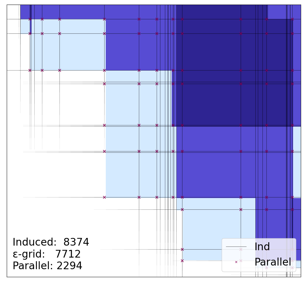
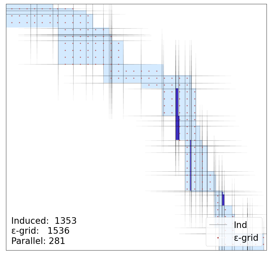
Our final algorithm, the parallel grid scan, blends this exact computation with the approximation to avoid the -bottleneck (Figure 13). We have implemented it and use it to demonstrate the applicability of the Skyscraper Invariant in data analysis by computing filtered Multiparameter Landscapes for biological data from [61].
Related Work.
Many informative invariants of MPM have been proposed in the literature, including, among others, [9, 8, 41, 48, 53, 2], and for some, there are also implemented algorithms [21, 60, 16, 13, 47, 45, 62]. All of these are either not stronger than the rank invariant, not (yet) practically computable for large modules, or unstable in interleaving distance, demonstrating the advantage of our work. The idea of computing filtrations has also appeared in [7, 52]. An algorithm for the Skyscraper Invariant has been implemented in the special case of ladder persistence modules [37]. The computation of HN filtrations of quiver representations is an active topic in complexity theory [35, 30].
1 The Skyscraper Invariant for Multiparameter Persistence Modules
Multiparameter Persistence.
Topological Data Analysis seeks to compute topological invariants from geometric data. In a typical setting, one constructs a simplicial complex filtered by a map . The sublevel sets assemble to a functor via inclusion. Composition with homology over a fixed field yields a functor - a Multiparameter Persistence Module.
The most important use case in practice are density-scale bifiltrations:
Example 2.
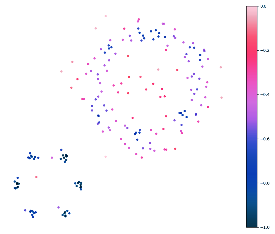
A standard 1-parameter pipeline [22] on a point set looks as follows: One constructs the Vietoris-Rips complex, filtered by one parameter, and computes its first persistent homology group, which decomposes into a barcode or persistence diagram (Figure 2).
The large circle on the right is impossible to detect with this technique without knowing the intensity of the noise we need to remove. Instead, we filter the simplicial complex again.
Intervals.
The analog of a bar in the multiparameter case is the Interval Module.
Definition 3 (Interval Module).
A sub poset is an interval if, with respect to the order, it is convex and connected. The module is defined as
An interval module is a persistence module that is isomorphic to for some interval .
Motivation.
The Skyscraper Invariant arises from the Harder-Narasimhan filtration [31] of persistence modules for a specific set of stability conditions. We will explain how one could arrive at considering HN filtrations even without prior knowledge of geometric invariant theory [54]. This theory was originally developed for persistence modules in [27] and [26].
Lifetime.
Let be a multiparameter persistence module. A sensible idea to extend the barcode is the following: search for an element with a "maximal lifetime" (an idea developed further in [52]). By "lifetime", we mean for any element , with , the set
of parameter values under which persists and "maximal" refers here to its volume. To assure that every lifetime has a finite volume, we will assume that every module is bounded, which can always be realised by restricting the module to a bounded subset of .
Example 4.
Consider again the bifiltered simplicial complex obtained from the point set from Figure 2 filtered by a kernel density estimate. The 2-parameter module produced by can be visualized by its Hilbert function - the pointwise dimension, which we denote by .
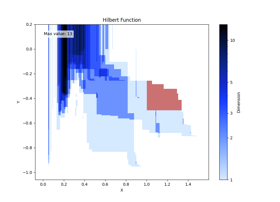
There is a non-zero vector at corresponding to the large circle in after filtering out points of density lower than . We mark its lifetime red in Figure 4.
After finding the vector of maximal lifetime, the submodule of generated by is an interval module and is the support of . Hence, if we compute the quotient , and repeat this process, we obtain a filtration of in terms of interval modules.
Additivity.
The element of maximal lifetime is not compatible with direct sums of modules.
Example 5.
Consider now Figure 5, where we return to the module from Figure 3. It can be split into two indecomposable summands, each roughly corresponding to one circle in the point set. The element of maximal lifetime is the vector .
If we instead consider the minimal lifetime of an element, the construction becomes additive, meaning the desired vector lies in a direct summand:
| (1) |
This enables the use of decomposition algorithms (e.g. [20]) to speed up the search. Now, a priori, this element is not well defined, since in every non-zero persistence module we can find a sequence of elements whose lifetime approaches a set of empty volume. To fix this, we choose a concrete parameter value and demand that the element be in .
Definition 6.
Let be a subset of . We denote by its induced submodule.
Since we are only considering elements at , we can now restrict our computations to – and this module is simpler than :
Definition 7.
is uniquely generated if it has a set of generators of the same degree.
In particular, is more decomposable than . Still, the choice of an element is not unique: there could be multiple vectors whose lifetime has the same (minimal) volume. This is the first hint that one should not only consider single elements in , but instead consider submodules of arbitrary dimension generated at a parameter value .
Stability.
Let be any sub vector space. The integral of the Hilbert function over would be the natural generalisation of the volume of the lifetime. However, using this definition would never make a subvector space of dimension higher than be the candidate for minimal lifetime. We need to average over the dimension of .
Definition 8.
The maximal submodule of highest slope is semistable. We define as the maximal submodule of highest slope in and continue iteratively. This produces a sequence of semistable modules . By defining inductively , we arrive at the Harder-Narasimhan-filtration [31]
| (2) |
of by [26, Theorem (A)]. The semistable modules are by definition isomorphic to the factors . The sequence of slopes is decreasing in , but this is not obvious. For a formal treatment, see [26] and [28, §2.4].
Example 9.
In Figure 6, we construct a semistable module that is not an interval.
At , each of the three shown submodules has slope . Every other dimension subspace has a lifetime equal to the whole support of the module and therefore slope . The whole module on the other hand has slope , so it is semistable.
Because of the existence of modules like Section 1, the factors of the Harder-Narasimhan filtration at should generally not all be intervals. Surprisingly, they did turn out to be intervals for all of our examples of density-scale bifiltrations of point sets in .
Conjecture 10.
Let be a finite point set and be any density-scale bifiltration of . All indecomposable uniquely generated submodules of are intervals.
Then, in particular, all factors of the Harder-Narasimhan filtration are intervals by additivity.
The Skyscraper Invariant.
Let be the HN filtration at .
Definition 11.
[26] For and , the Skyscraper Invariant is
This value only depends on the Hilbert function of the factors . Since , the Skyscraper Invariant filters the rank invariant.
Example 12.
The modules and cannot be distinguished by the rank invariant.
Distances.
Approximation.
Given for all in a grid , we can define the functor over via a projection to the next lower element in .
Lemma 13 ([28, Lemma 3.4]).
If -approximates , then .
Intervals and Data Structures.
After computing the HN filtrations, we need to store the Hilbert functions of the filtration factors and their associated slopes. The Hilbert functions of each factor can be stored as a list of intervals, , each being assigned the slope of . For each , this results in a list of at most intervals. To compute from this list, we count how many with an associated slope greater than contain . The latter can be done in time where is the number of relations of the interval. Since , This puts the query time in .
Presentations.
The data structure in which persistence modules come is that of a presentation. This is a set of generators and a set of relations among the generators. They are collected in a matrix where each row corresponds to a generator and each column to a relation. The rows and columns are endowed with the parameter value – or degree – of the corresponding generator or relation, making this a graded matrix or monomial matrix [49]. If we write for the free module generated by a tuple of degrees , then a graded matrix is nothing but a linear map and it presents iff .
Each finitely encoded persistence modules [51] has a finite minimal presentation which can be extended to a minimal resolution. The degrees of the generators, relations, higher relations etc. in a minimal resolution are independent of the chosen resolution and form multi-subsets – the graded Betti numbers of . We denote the category of bounded finitely presented persistence modules by .
2 Computing the Skyscraper Invariant Approximately
Our definition of the HN filtration given in the previous section is actually not consistent with the classical one [31, 42]. Instead of a filtration of one really considers a filtration of . Only by the observation [26, Proposition 3.3] it actually restricts to one of . The first simplification in our algorithms is the computation of this submodule .
Induced Submodules.
Computing a presentation for any induced submodule can be done by computing the kernel of a graded matrix in the category of persistence modules. For , this can be done with the LWKR-algorithm (Lesnick, Wright, Kerber, and Rolle [43, 40]) and for there is an unpublished algorithm [5] by Bender, Gäfvert, and Lesnick. When is larger, we rely on classical machinery, like Schreyer’s algorithm [23], which is too slow in practice. We will therefore focus on the -parameter case for this paper.
Proposition 14.
1 computes a presentation of .
Proof.
See [28, Proposition 3.1] for a chase in the following diagram:
Approximate Computation.
We condense the ideas from Section 1 into an algorithm.
Correctness.
Denote by the input size, the thickness of , the maximal thickness of a uniquely generated indecomposable submodule, and by , , and the times to compute the HN filtration, kernels, and decomposition for -parameter modules.
Proposition 15.
2 returns an -approximation of the Skyscraper Invariant in
Proof.
Correctness follows from additivity (Equation 1) and the fact that we only need the ordered list of Hilbert functions of factors. At each step there are at most indecomposable submodules of thickness generated at .
3 Finding Highest-Slope Submodule
We will explain how to compute the Harder-Narasimhan filtration of with an exhaustive search. To do so, we must compute slopes. The slope at is entirely determined by the Hilbert function of and thus by its Betti numbers.
Proposition 16.
Let , then
| (3) |
Proof.
Consider a minimal free resolution which will be of maximal length by Hilbert’s Syzygy theorem. In our bounded case, it will even be exactly of length by duality of free and injective resolutions (first proved by Miller in [50] and rediscovered in [3] for the computation of Multiparameter Persistent Cohomology). Each has a basis with degrees at . By exactness, for each we have
| (4) |
Let be large enough that , then
| (5) |
As a function of , Equation 5 is a polynomial and constant, so we can set .
Iteration over subspaces.
Instead of considering , we assume without loss of generality, that is uniquely generated at . Recall that , and choose any basis . We want to find the sub vector space for which has the highest slope. An exhaustive search would involve computing with Algorithm 1 for all sub vector spaces . This is clearly possible if we work over a finite field, but also in the infinite case, the finite presentation of allows only a finite number of non-isomorphic submodules. Since all software uses finite fields, we fix a prime power and .
Denote by the set of 1-dimensional subspaces of and define
Proposition 17.
Let and define . If for every -subspace it holds that , then has a higher slope than any other submodule of thickness .
Proof.
Consider any of dimension . By assumption, there is a -dimensional subspace which is not in . Therefore, .
Every -dimensional vector space over contains exactly subspaces of dimension , so the premise of Section 3 is trivially satisfied if . has subspaces, but only of these are -dimensional.
Proposition 18.
3 returns the correct result in time.
Proof.
Correctness follows from Section 3 and Section 3. Algorithm 1 computes a kernel for each subspaces of , of which there are .
By calling Algorithm 3 recursively on the quotient by the submodule of highest slope we can compute the whole HN filtration at in time.
4 Cheng’s Algorithm
Building on the work of [19, 33], Cheng reduced the computation of HN filtrations of representations of finite acyclic quivers to the shrunk subspace problem, which can be solved in deterministic polynomial-time for large enough fields [15]. This algorithm can be directly applied to persistence modules over a finite poset [26, Remark 1.13].
It does not follow directly from Section 1 that computing the HN filtration after restriction to the grid produces an error on less than in the erosion distance, because this could change which submodule has the highest slope. Instead, one needs to apply the functoriality of the HN filtration [24] on an interleaving [26, Theorems 2.9 and 3.7].
Shrunk subspace problem.
Fix two integers and a field . The space of matrices with coefficients in is denoted and we write for the Kronecker product.
Definition 19 (shrunk subspace).
Let be a subspace. A subspace
Observe that the being a shrunk subspace of is closed under intersections. We can thus define the minimal shrunk subspace of .
For the purpose of this paper, we present a simple random algorithm introduced in [29, Theorem 6.7] for . We extend this algorithm to any field using [34, Lemma 5.3]
Proposition 20.
Fix a field and . Given an integer and a subspace generated by a family of matrices, there exists a random algorithm to compute the minimal shrunk subspace of using at most arithmetic operations for some constant .
From persistence module to shrunk subspace.
Fix and a number . Assume that the support of is contained in a bounded cube and let . We denote by the restriction of to . Using the Persistence-Algebra library one can compute the structure maps of in time .
Let , and let . Define and . Consider the following subspace of :
| (6) |
Proposition 21 ([36, Theorem 4.3]).
Let and let be the HN filtration of at . Let be the maximum integer
The minimal shrunk subspace of is .
Cheng also observed in the above Theorem that when , either or [15, Corollary 3.4]. They thus devised Algorithm 4.
Corollary 22.
Given and , there is a random algorithm to compute an -approximation of in time up to poly-logarithmic factors.
Proof.
By [26] (as detailed in [28, Corollary 4.5]), applying for every Algorithm 4 to the restriction of to yields an -approximation of . By Section 4 with and , line 3 in Algorithm 4 takes for any . The recursive step adds a factor , whence the desired complexity.
Improvements to Cheng’s algorithm.
By harnessing the block structure of (6), we are able to improve the complexity in Section 4 for the subspaces appearing in Algorithm 4.
Proposition 23.
Given and , there is a random algorithm to compute an -approximation of in time up to poly-logarithmic factors.
Further empirical improvements can be obtained by computing in Section 4 for small integers such that . Indeed, the complexity of computing is heavily dependent on the size of . For simplicity, assume that . If , then we can replace by in Algorithm 4. Otherwise, we know that there are no submodule such that . We keep choosing better approximations of (so with higher values of ) until either we find a proper submodule in the HN filtration of at , or we can guarantee that is semistable at .
Finally, given and a matrix , our implementation uses the block structure of to partially reduce it: Since for some , we column-reduce the first block rows of by reducing and each .
These two empirical improvements led to significant speed-ups (see [28, Table 3]).
5 Exact Computation of the Skyscraper Invariant
The slope in relation to .
For many computations on persistence modules, it is often enough to perform them only at those parameter values that share each of their coordinates with a generator or relation (cf. the barcode template [43, 44]). We call the set of these parameters, , the induced grid of . It partitions into rectangular cells.
Consider any cell in the grid on the left in Figure 8, which is slightly coarser than the induced grid. For all , the submodules will look qualitatively similar: Each has a presentation with the same underlying matrix. We will use this fact to avoid recomputing decompositions and HN filtrations for every on an -grid.
For , denote by the hyperplane spanned by the coordinate axes indicated by , with the origin at . The graded Betti numbers, which lie in some for , will be shifted to align with when changes (Figure 9).
Lemma 24.
Let be generated at . For in the first cell of , the function is a multilinear polynomial of degree which we denote by and
| (7) |
In particular, the leading coefficient is and the constant term is .
Proof by picture: Figure 10.
Full proof in [28, Lemma 6.5]
Observation 25.
To find the submodule of highest slope for all in a grid cell at the same time, compute the lower envelope of the slope polynomials of all non-isomorphic submodules. Since they have the same leading term we can omit it for the computation of this diagram. For the important case of , this is the lower envelope of a set of planes in and can be computed efficiently as the upper convex hull of its dual point set [18, 14.2].
We describe this computation for , where after ignoring the degree- part, the slope-polynomials are linear and so the minimisation diagram is convex-polygonal.
The thickness- module from Table 1 produces the following subdivision.
Arrangements.
We ran Algorithm 5 for all modules used in Table 1. In each case, as in Figure 11, the first grid cell lies entirely in one face of the subdivision.
Proposition 26.
5 is correct and runs in expected time .
Proof.
Correctness follows from Section 5 and Section 5. The runtime is the same as for Algorithm 3, except that kernel computation is in for 2-parameter modules and we compute a lower envelope. That can be done in expected time , putting the runtime in
Exact Computation of the Skyscraper Invariant.
For each , there is a highest-slope submodule associated with the face . By computing the quotient and recursively calling Algorithm 5 on the pair , we obtain a nested sequence of subdivisions of the grid cell and an associated tree of filtration factors. Glueing these for all grid cells, we obtain a data structure from which we can compute the exact value of by locating in the nested subdivisions [28, Section 6.4].
Wall and Chamber Structure.
For all in a region of this nested sequence of subdivisions, the module has equivalent HN filtrations. This is one implication of Theorem 1.
Parallel grid scanning: The final algorithm.
In practice, where one wants to compute filtered vectorisations of the Skyscraper Invariant, it is not a problem to restrict the module to an -grid and use Algorithm 2. The real power of Theorem 1 and Algorithm 5 lies in the fact that it is a recipe to avoid recomputations: For any direct summand of the input module, the induced grid is typically coarser than in some places and finer than in others. We therefore overlay the two grids to form the restriction or parallel grid and use Algorithm 5 only for those cells in each that intersect . This technique enables fast computation of the Skyscraper Invariant at high resolution.
6 Experiments
All experiments are performed on an i7-1255U Processor without any parallelisation. A timeout was set to min and each run is averaged over instances whenever possible. Our software and experiments are built using the Persistence-Algebra C++ library222https://github.com/JanJend/Skyscraper-Invariant,
https://github.com/JanJend/Persistence-Algebra.
Harder-Narasimhan filtrations.
To generate indecomposable uniquely generated submodules of non-zero thickness we used synthetically generated noisy samples of a torus embedded in (cf Section 1) and random presentation matrices. We test the exhaustive search Algorithm 3 and its filter Section 3. For thickness , Algorithm 3 always timed out.
| Dataset | Variant | 2 | 3 | 4 | 5 | 6 | 7 | 8 |
|---|---|---|---|---|---|---|---|---|
| Torus | with filter | 2.2 | 2.8 | 5.5 | 19.5 | 202 | 2.7k | – |
| Torus | w/o filter | 2.8 | 2.8 | 5.3 | 18.8 | 206 | 2.7k | – |
| Random | with filter | 8.1 | 4.8 | 6.4 | 28.9 | 454 | 5.9k | 100k |
| Random | w/o filter | 3.6 | 2.3 | 5.1 | 27.1 | 265 | 3.6k | 61.5k |
We conclude that the filter (Section 3) for Algorithm 3 is barely helpful.
Runtime of Cheng’s algorithm.
After restricting the torus generated modules to equidistant grids, we have used Cheng’s algorithm (Algorithm 4) over and . Since we can only generate modules from bifiltrations over , we interpreted them as -modules when possible.
| 2 | 3 | 4 | 5 | 6 | 7 | |
|---|---|---|---|---|---|---|
| 2x2 | 1.9/1.8 | 1.8/3.0 | 1.8/4.3 | 5.0/5.0 | 4.4/10.3 | 11.6/33.4 |
| 3x3 | 8.7/18.5 | 15.2/27.4 | 21.8/43.2 | 76.6/157k* | 40.8/3.7k | 53.0/301 |
| 4x4 | 113/2.0k | 1.1k/117k* | 412/223* | 720/33.6k | 499/66.6k | 177/38.4k* |
| 5x5 | 1.8k/154k* | 11.8k/283* | 36.8k/279k* | 11.3k/– | 5.2k/254k* | 2.7k/– |
| 6x6 | 61.5k/– | 205k/– | 323k/– | 39.4k/– | 66.6k/– | 16.1k/– |
We observe a great variability of runtimes for Cheng’s algorithm depending on whether the heuristic introduced at the end of Section 4 successfully computes and certifies the correctness of all the HN filtrations. The random algorithm from [30] performs computations on square matrices with rows for a large enough . For (but not for ), we have observed in our experiments that is large enough.
Comparison.
Table 2 shows the strong dependence of Algorithm 4 on the size of the grid to which the uniquely graded module has to be restricted. Algorithm 3 does not require this restriction but, as visible in Table 1, it is highly dependent on the thickness of the input.
The asymptotic runtimes of the algorithms suggest that for practical grids , Cheng’s algorithm would outperform the exhaustive search not before . At that point, the number of arithmetic operations is too large for any computer to handle.
Runtime on practical data.
We used benchmark data from [39, 61] to compare the parallel grid scan algorithm with Algorithm 2.
| Data | Circle | D7.5k | D15k | D30k | MC46 | MC96 | MC175 |
|---|---|---|---|---|---|---|---|
| n | 100 | 140 | 219 | 333 | 3.3k | 9.1k | 19.6k |
| Parallel | 0.03 | 0.16 | 0.42 | 1.25 | 0.08 | 0.41 | 1.45 |
| Alg 2 | 1.87 | 0.47 | 0.41 | 0.76 | 12.68 | 32.97 | 73.54 |
The parallel grid scan should not show the same quadratic dependency on the grid size of Algorithm 2. Table 4 confirms this and shows that our algorithm computes the Skyscraper Invariant in a practical timeframe for relevant data sizes.
| Data | uni , | uni , | Hyp | Hyp | Hyp | Hyp |
|---|---|---|---|---|---|---|
| n | 113k | 93.5k | 9.4k | 9.4k | 9.4k | 9.4k |
| Parallel | 299.7 | 422.0 | 54.8 | 93.4 | 167.5 | 311.3 |
7 Application and Conclusion
Filtered Landscapes.
The Multiparameter Landscape [60] is directly defined by the ranks of the diagonal maps . Therefore, we can filter the Landscape by replacing the rank with the Skyscraper Invariant. As an example, we will use the IHC stained sample LargeHypoxicRegion1 of a tumour, for which the authors of [61] analyse the location of immune cells using Multiparameter Landscapes.
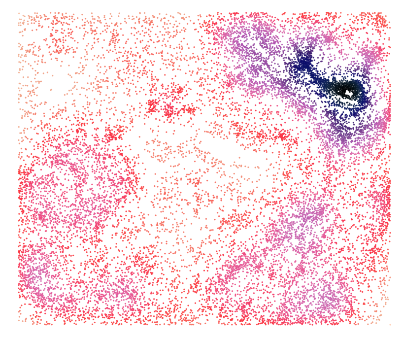
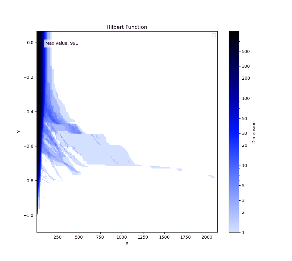
Using multipers [46], we computed its density-alpha bifiltration with function-delaunay [63], a minimal presentation of the first persistent homology group thereof with mpfree [40], and restricted it to a grid. Computing the Skyscraper Invariant on this matrix took around 5 minutes.
Since the filtered Landscapes are stable [26, Corollary 3.12], their differences are too, revealing elements of long lifetime.
Conclusion.
With our algorithms and the induced filtered Landscapes practitioners have a new invariant for topological data analysis that is robust to noise, finer than the rank invariant, efficiently computable, and is interpretable directly from its visual representation.
Open Problems.
To incorporate invariants into Machine Learning pipelines, the authors of [58] define a framework which needs to be extended to include the Skyscraper Invariant. Instead of Landscapes, one can also filter other vectorizations of the rank invariant. By changing the stability condition [26], we obtain different HN filtrations and invariants. Can our methods be adapted to this general setting?
References
- [1] Ethan André, Jingyi Li, David Loiseaux, and Steve Oudot. Estimating the persistent homology of -valued functions using function-geometric multifiltrations, 2025. arXiv:2412.04162.
- [2] Hideto Asashiba. Relative koszul coresolutions and relative betti numbers. Journal of Pure and Applied Algebra, 229(3):107905, 2025. doi:10.1016/j.jpaa.2025.107905.
- [3] Ulrich Bauer, Fabian Lenzen, and Michael Lesnick. Efficient Two-Parameter Persistence Computation via Cohomology. In Erin W. Chambers and Joachim Gudmundsson, editors, 39th International Symposium on Computational Geometry (SoCG 2023), volume 258 of Leibniz International Proceedings in Informatics (LIPIcs), pages 15:1–15:17, Dagstuhl, Germany, 2023. Schloss Dagstuhl – Leibniz-Zentrum für Informatik. doi:10.4230/LIPIcs.SoCG.2023.15.
- [4] Ulrich Bauer and Luis Scoccola. Multi-parameter persistence modules are generically indecomposable. International Mathematics Research Notices, 2025(5):rnaf034, February 2025. doi:10.1093/imrn/rnaf034.
- [5] Matías Bender, Oliver Gäfvert, and Michael Lesnick. Computing minimal presentations of multi-parameter persistent homology, 2023. URL: https://github.com/MBender/muphasa.
- [6] Katherine Benjamin, Aneesha Bhandari, Jessica D. Kepple, Rui Qi, Zhouchun Shang, Yanan Xing, Yanru An, Nannan Zhang, Yong Hou, Tanya L. Crockford, Oliver McCallion, Fadi Issa, Joanna Hester, Ulrike Tillmann, Heather A. Harrington, and Katherine R. Bull. Multiscale topology classifies cells in subcellular spatial transcriptomics. Nature, 630(8018):943–949, June 2024. doi:10.1038/s41586-024-07563-1.
- [7] Håvard Bakke Bjerkevik. Stabilizing decomposition of multiparameter persistence modules. Foundations of Computational Mathematics, January 2025. doi:10.1007/s10208-025-09695-w.
- [8] Benjamin Blanchette, Thomas Brüstle, and Eric J. Hanson. Exact structures for persistence modules. In Lidia Angeleri Hügel, Bernhard Keller, María Julia Redondo, and Andrea Solotar, editors, Representations of Algebras and Related Topics, pages 121–160. European Mathematical Society Publishing House, 2022. doi:10.4171/ECR/21/4.
- [9] Magnus Bakke Botnan, Steffen Oppermann, and Steve Oudot. Signed Barcodes for Multi-Parameter Persistence via Rank Decompositions. In International Symposium on Computational Geometry (SoCG), 2022. doi:10.4230/LIPIcs.SoCG.2022.19.
- [10] Tom Bridgeland. Stability conditions on triangulated categories. Annals of Mathematics, 166:317–345, 2007. doi:10.4007/annals.2007.166.317.
- [11] Gunnar Carlsson and Afra Zomorodian. The theory of multidimensional persistence. Discrete and Computational Geometry, 42:71–93, June 2007. doi:10.1007/s00454-009-9176-0.
- [12] Gunnar E. Carlsson and Afra Zomorodian. The theory of multidimensional persistence. In The ACM Symposium on Computational Geometry (SoCG), 2007. doi:10.1145/1247069.1247105.
- [13] Mathieu Carrière and Andrew J. Blumberg. Multiparameter persistence images for topological machine learning. In Proceedings of the 34th International Conference on Neural Information Processing Systems, NIPS ’20. Curran Associates Inc., 2020. URL: https://proceedings.neurips.cc/paper_files/paper/2020/hash/fdff71fcab656abfbefaabecab1a7f6d-Abstract.html.
- [14] Frédéric Chazal, David Cohen-Steiner, Marc Glisse, Leonidas J Guibas, and Steve Y Oudot. Proximity of persistence modules and their diagrams. In Proceedings of the twenty-fifth annual symposium on Computational geometry, pages 237–246, 2009. doi:10.1145/1542362.1542407.
- [15] Chi-Yu Cheng. A deterministic algorithm for Harder-Narasimhan filtrations for representations of acyclic quivers. Algebra & Number Theory, 18(2):319–347, 2024. doi:10.2140/ant.2024.18.319.
- [16] René Corbet, Ulderico Fugacci, Michael Kerber, Claudia Landi, and Bei Wang. A kernel for multi-parameter persistent homology. Computers & Graphics: X, 2, 2019. doi:10.1016/j.cagx.2019.100005.
- [17] René Corbet, Michael Kerber, Michael Lesnick, and Georg Osang. Computing the multicover bifiltration. Discrete & Computational Geometry, 70(2):376–405, September 2023. doi:10.1007/s00454-022-00476-8.
- [18] Mark de Berg, Otfried Cheong, Marc van Kreveld, and Mark Overmars. Computational Geometry: Algorithms and Applications. Springer, Berlin, 3 edition, 2008.
- [19] Harm Derksen and Visu Makam. Polynomial degree bounds for matrix semi-invariants. Advances in Mathematics, 310:44–63, 2017. doi:10.1016/j.aim.2017.01.018.
- [20] Tamal K. Dey, Jan Jendrysiak, and Michael Kerber. Decomposing Multiparameter Persistence Modules. In Oswin Aichholzer and Haitao Wang, editors, 41st International Symposium on Computational Geometry (SoCG 2025), volume 332 of Leibniz International Proceedings in Informatics (LIPIcs), pages 41:1–41:19, Dagstuhl, Germany, 2025. Schloss Dagstuhl – Leibniz-Zentrum für Informatik. doi:10.4230/LIPIcs.SoCG.2025.41.
- [21] Tamal K. Dey, Woojin Kim, and Facundo Mémoli. Computing generalized rank invariant for 2-parameter persistence modules via zigzag persistence and its applications. In International Symposium on Computational Geometry (SoCG), 2022. doi:10.4230/LIPIcs.SOCG.2022.34.
- [22] Herbert Edelsbrunner, David Letscher, and Afra Zomorodian. Topological persistence and simplification. In Proceedings 41st annual symposium on foundations of computer science, pages 454–463. IEEE, 2000. doi:10.1007/s00454-002-2885-2.
- [23] Burçin Eröcal, Oleksandr Motsak, Frank-Olaf Schreyer, and Andreas Steenpaß. Refined algorithms to compute syzygies. Journal of Symbolic Computation, 74:308–327, 2016. doi:10.1016/j.jsc.2015.07.004.
- [24] Gerd Faltings. Mumford-stabilität in der algebraischen geometrie. In S. D. Chatterji, editor, Proceedings of the International Congress of Mathematicians, pages 648–655, Basel, 1995. Birkhäuser Basel.
- [25] Marc Fersztand. Cheng’s algorithm for persistence modules over finite posets. Software, version 0.1., EPSRC grant EP/R018472/1., swhId: swh:1:dir:b620e11fefcb30adcafaf299484f00c1b0a2af70 (visited on 2026-05-18). URL: https://github.com/marcf-ox/sky-inv-quiv, doi:10.4230/artifacts.26093.
- [26] Marc Fersztand. Harder-narasimhan filtrations of persistence modules: metric stability, 2024. arXiv:2406.05069.
- [27] Marc Fersztand, Emile Jacquard, Vidit Nanda, and Ulrike Tillmann. Harder–Narasimhan filtrations of persistence modules. Transactions of the London Mathematical Society, 11(1):e70003, 2024. doi:10.1112/tlm3.70003.
- [28] Marc Fersztand and Jan Jendrysiak. Computing the skyscraper invariant, 2026. arXiv:2603.23560.
- [29] Cole Franks, Tasuku Soma, and Michel X Goemans. Shrunk subspaces via operator sinkhorn iteration, 2022. doi:10.48550/arXiv.2207.08311.
- [30] Cole Franks, Tasuku Soma, and Michel X Goemans. Shrunk subspaces via operator sinkhorn iteration. In Proceedings of the 2023 Annual ACM-SIAM Symposium on Discrete Algorithms (SODA), pages 1655–1668. SIAM, 2023. doi:10.1137/1.9781611977554.ch62.
- [31] Günter Harder and Mudumbai S. Narasimhan. On the cohomology groups of moduli spaces of vector bundles on curves. Mathematische Annalen, 212:215–248, 1974. doi:10.1007/BF01357141.
- [32] Lutz Hille and José Antonio de la Peña. Stable representations of quivers. Journal of Pure and Applied Algebra, 172(2):205–224, 2002. doi:10.1016/S0022-4049(01)00167-0.
- [33] Alana Huszar. Non-commutative rank and semi-stability of quiver representations, 2021. arXiv:2111.00039.
- [34] Gábor Ivanyos, Youming Qiao, and KV Subrahmanyam. Constructive non-commutative rank computation is in deterministic polynomial time. computational complexity, 27:561–593, 2018. doi:10.1007/s00037-018-0165-7.
- [35] Yuni Iwamasa, Taihei Oki, and Tasuku Soma. Algorithmic Aspects of Semistability of Quiver Representations. In 52nd International Colloquium on Automata, Languages, and Programming (ICALP 2025), volume 334 of Leibniz International Proceedings in Informatics (LIPIcs), pages 99:1–99:18. Schloss Dagstuhl – Leibniz-Zentrum für Informatik, 2025. doi:10.4230/LIPIcs.ICALP.2025.99.
- [36] Yuni Iwamasa, Taihei Oki, and Tasuku Soma. Algorithmic aspects of semistability of quiver representations, 2025. arXiv:2407.06493.
- [37] Emile Jacquard. Topics in multidimensional persistence. Phd thesis, University of Oxford, 2024. URL: https://ora.ox.ac.uk/objects/uuid:591b13e1-faab-4da2-a405-d986a629003a.
- [38] Jan Jendrysiak. Skyscraper Invariant and Filtered Multiparameter Landscapes. Software, version 0.1., swhId: swh:1:dir:8ed2562604075467f0b0014975100a2d26e434ba (visited on 2026-05-18). URL: https://github.com/JanJend/Skyscraper-Invariant, doi:10.4230/artifacts.26094.
- [39] Michael Kerber and Tung Lam. Benchmark data sets of minimal presentations of 2-parameter persistence modules [data set]. Graz University of Technology, 2025. doi:10.3217/rxedk-qyq77.
- [40] Michael Kerber and Alexander Rolle. Fast minimal presentations of bi-graded persistence modules. In Algorithm Engineering and Experiments (ALENEX), 2021. doi:10.1137/1.9781611976472.16.
- [41] Woojin Kim and Facundo Mémoli. Generalized persistence diagrams for persistence modules over posets. Journal of Applied and Computational Topology, 5(4):533–581, August 2021. doi:10.1007/s41468-021-00075-1.
- [42] A. D. King. Moduli of representations of finite dimensional algebras. The Quarterly Journal of Mathematics, 45(4):515–530, December 1994. doi:10.1093/qmath/45.4.515.
- [43] Michael Lesnick and Matthew Wright. Computing minimal presentations and bigraded betti numbers of 2-parameter persistent homology. SIAM Journal on Applied Algebra and Geometry, 6(2):267–298, 2022. doi:10.1137/20M1388425.
- [44] Michael Lesnick and Matthew Wright. Fast queries of fibered barcodes, 2025. arXiv:2511.05837.
- [45] David Loiseaux, Mathieu Carrière, and Andrew J Blumberg. Multi-parameter module approximation: an efficient and interpretable invariant for multi-parameter persistence modules with guarantees. Journal of Applied and Computational Topology, 9(4):1–60, 2025. doi:10.1007/s41468-025-00222-y.
- [46] David Loiseaux and Hannah Schreiber. Multipers: Multiparameter Persistence for Machine Learning. Journal of Open Source Software, 9(103):6773, November 2024. doi:10.21105/joss.06773.
- [47] David Loiseaux, Luis Scoccola, Mathieu Carrière, Magnus Bakke Botnan, and Steve Oudot. Stable vectorization of multiparameter persistent homology using signed barcodes as measures. In Advances in Neural Information Processing Systems (NeurIPS), 2023. URL: http://papers.nips.cc/paper_files/paper/2023/hash/d75c474bc01735929a1fab5d0de3b189-Abstract-Conference.html.
- [48] Alexander McCleary and Amit Patel. Edit distance and persistence diagrams over lattices. SIAM Journal on Applied Algebra and Geometry, 6(2):134–155, 2022. doi:10.1137/20M1373700.
- [49] Ezra Miller. The alexander duality functors and local duality with monomial support. Journal of Algebra, 231(1):180–234, 2000. doi:10.1006/jabr.2000.8359.
- [50] Ezra Miller. Graded greenlees–may duality and the čech hull. In Local Cohomology and Its Applications, volume 226 of Lecture Notes in Pure and Applied Mathematics, pages 233–253. Marcel Dekker, 2001. doi:10.1201/9781482275766.
- [51] Ezra Miller. Data structures for real multiparameter persistence modules, 2020. arXiv:1709.08155.
- [52] Ezra Miller and Jiaxi Zhang. Lifetime filtration of multiparameter persistence modules, 2024. Presentation for Spires 2024, Oxford. URL: https://sites.math.duke.edu/˜ezra/Talks/horizons-in-alg-for-multiPH.pdf.
- [53] Dmitriy Morozov and Amit Patel. Output-sensitive computation of generalized persistence diagrams for 2-filtrations, 2023. arXiv:2112.03980.
- [54] David Mumford, John Fogarty, and Frances Kirwan. Geometric Invariant Theory, volume 34 of Ergebnisse der Mathematik und ihrer Grenzgebiete. Springer-Verlag, 3 edition, 1994.
- [55] Amit Patel. Generalized persistence diagrams. Journal of Applied and Computational Topology, 1(3):397–419, 2018. doi:10.1007/s41468-018-0012-6.
- [56] Ville Puuska. Erosion distance for generalized persistence modules. Homology, Homotopy & Applications, 22(1), 2020. doi:10.4310/HHA.2020.v22.n1.a14.
- [57] Gian Carlo Rota. On the foundations of combinatorial theory i. theory of möbius functions. Zeitschrift für Wahrscheinlichkeitstheorie und Verwandte Gebiete, 2(4):340–368, January 1964. doi:10.1007/BF00531932.
- [58] Luis Scoccola, Siddharth Setlur, David Loiseaux, Mathieu Carrière, and Steve Oudot. Differentiability and optimization of multiparameter persistent homology. In Proceedings of the 41st International Conference on Machine Learning, ICML’24. JMLR.org, 2024. URL: https://proceedings.mlr.press/v235/scoccola24a.html.
- [59] Donald R. Sheehy. A multicover nerve for geometric inference. In CCCG: Canadian Conference in Computational Geometry, pages 309–314, 2012. URL: http://2012.cccg.ca/papers/paper52.pdf.
- [60] Oliver Vipond. Multiparameter persistence landscapes. Journal of Machine Learning Research, 21:1–38, 2020. URL: http://jmlr.org/papers/v21/19-054.html.
- [61] Oliver Vipond, Joshua A Bull, Philip S Macklin, Ulrike Tillmann, Christopher W Pugh, Helen M Byrne, and Heather A Harrington. Multiparameter persistent homology landscapes identify immune cell spatial patterns in tumors. Proceedings of the National Academy of Sciences, 118(41), October 2021. doi:10.1073/pnas.2102166118.
- [62] Cheng Xin, Soham Mukherjee, Shreyas N. Samaga, and Tamal K. Dey. GRIL: A -parameter persistence based vectorization for machine learning. In Workshop on Topology, Algebra, and Geometry in Machine Learning (TAG-ML), pages 313–333, 2023. URL: https://proceedings.mlr.press/v221/xin23a.html.
- [63] Ángel Javier Alonso, Michael Kerber, Tung Lam, and Michael Lesnick. Delaunay bifiltrations of functions on point clouds. In Proceedings of the 2024 Annual ACM-SIAM Symposium on Discrete Algorithms (SODA), pages 4872–4891, 2024. doi:10.1137/1.9781611977912.173.