Constructing Doppelgängers of Greedy Geometric Spanners in Practice

Abstract
Greedy geometric spanners are considered to be the gold standard for their near-optimal guarantees in terms of sparsity and total weight. However, their inefficient construction poses significant challenges for large-scale geometric networks, especially for low values of stretch factors . We present -Greedy, a simple and practical parallel algorithm engineered for constructing doppelgängers of greedy geometric spanners that empirically resemble the greedy spanners in key structural and performance metrics, including average degree, degree, and lightness. Unlike approximate greedy spanners, doppelgängers of greedy spanners are almost indistinguishable from the actual greedy spanners in practice.
In our experiments, -Greedy consistently produced greedy spanner doppelgängers across a broad range of synthetic and real-world datasets, offering the first practical alternative to the computationally intensive greedy spanners. -Greedy can construct a -spanner on a -element uniformly distributed point set in well under 5 minutes. In contrast, Bucketing, the most practical greedy spanner algorithm, takes around 3 hours. For million-sized point sets, -Greedy can run to completion in a few hours, making it much faster than Bucketing, which takes days to finish. In extensive experiments on synthetic and real-world datasets, -Greedy delivered speedups of up to 147x over Bucketing while preserving greedy-like sparsity and weight.
For broader uses of the algorithm and reproducibility, we share our engineered C++ code.
Keywords and phrases:
geometric graph, geometric spanners, greedy spanners, algorithm engineeringCopyright and License:
![[Uncaptioned image]](x1.png) © Anirban Ghosh; licensed under Creative Commons License CC-BY 4.0
© Anirban Ghosh; licensed under Creative Commons License CC-BY 4.0
2012 ACM Subject Classification:
Theory of computation Computational geometryAcknowledgements:
The author would like to thank the anonymous reviewers for their insightful comments and suggestions, which helped to significantly improve the clarity and quality of this paper.Editors:
Hee-Kap Ahn, Michael Hoffmann, and Amir NayyeriSeries and Publisher:
 Leibniz International Proceedings in Informatics, Schloss Dagstuhl – Leibniz-Zentrum für Informatik
1 Introduction
A geometric spanner on a set of points in metric is a sparse subgraph of the complete Euclidean graph on that approximately preserves pairwise distances among all point pairs in . Formally, given a set of points and a stretch factor , a geometric graph is a -spanner if, for all , the shortest-path distance in , denoted by , satisfies , where denotes the Euclidean distance between . A -spanner is also a -spanner, for all . A -path exists between two points in a geometric graph if . Therefore, is a -spanner if for every point pair in , a -path exists in . The average degree of is defined as , and its lightness is the ratio of the weight of to the weight of a Euclidean minimum spanning tree of . For a fixed value of , lower average degree and lightness are better. The complete Euclidean graph is a 1-spanner with edges, rendering it impractical for large-scale applications. So, the study of geometric spanners focuses on designing algorithms that construct sparse -spanners, ideally with edges, while maintaining desirable geometric and algorithmic properties; see [13, 28, 34] for a comprehensive overview. Spanners play a central role in computational geometry and the design of geometric networks. They are widely used in applications such as wireless networks, motion planning, and approximation algorithms, where maintaining low stretch with minimal edge cost is essential [5, 18, 24, 27, 30, 31].
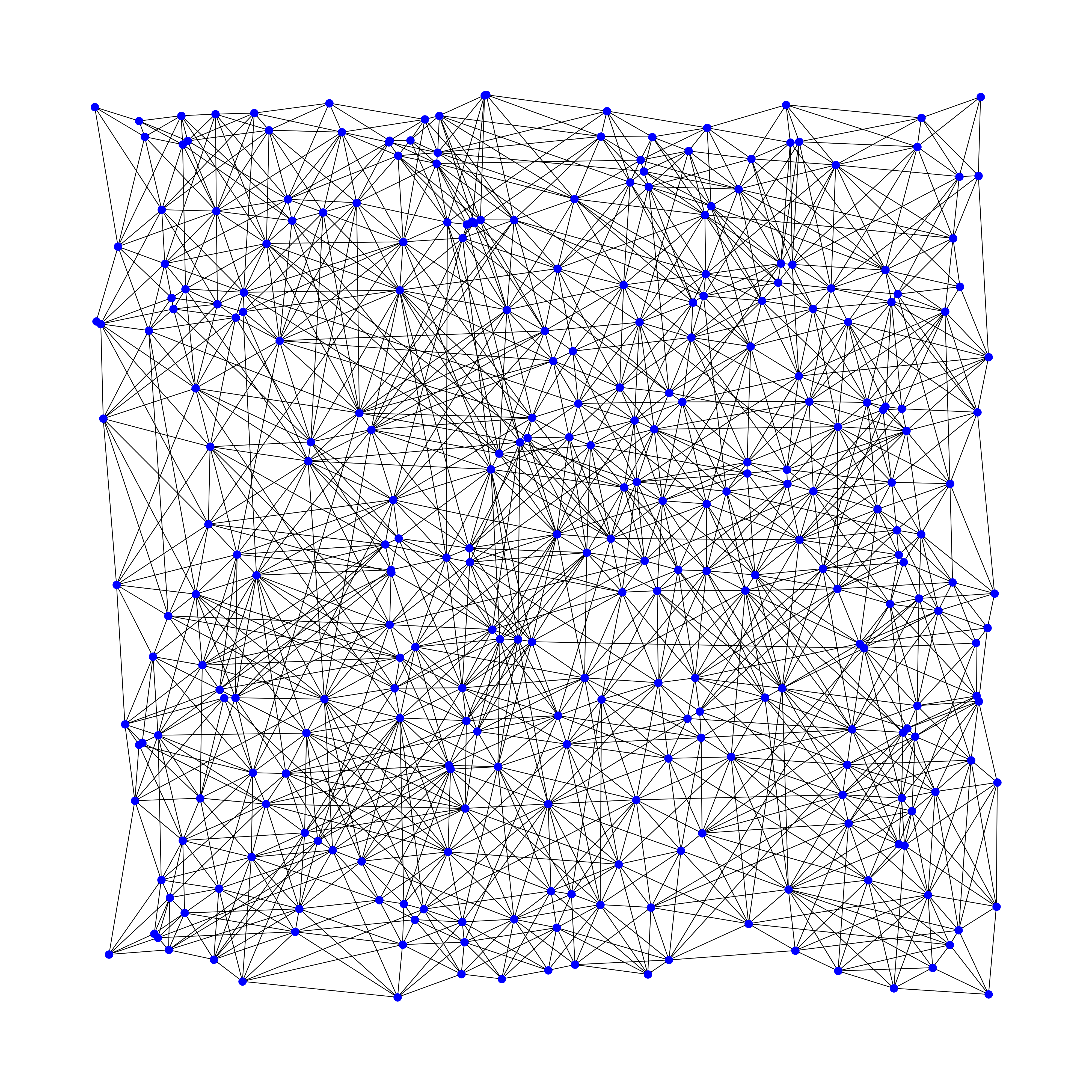
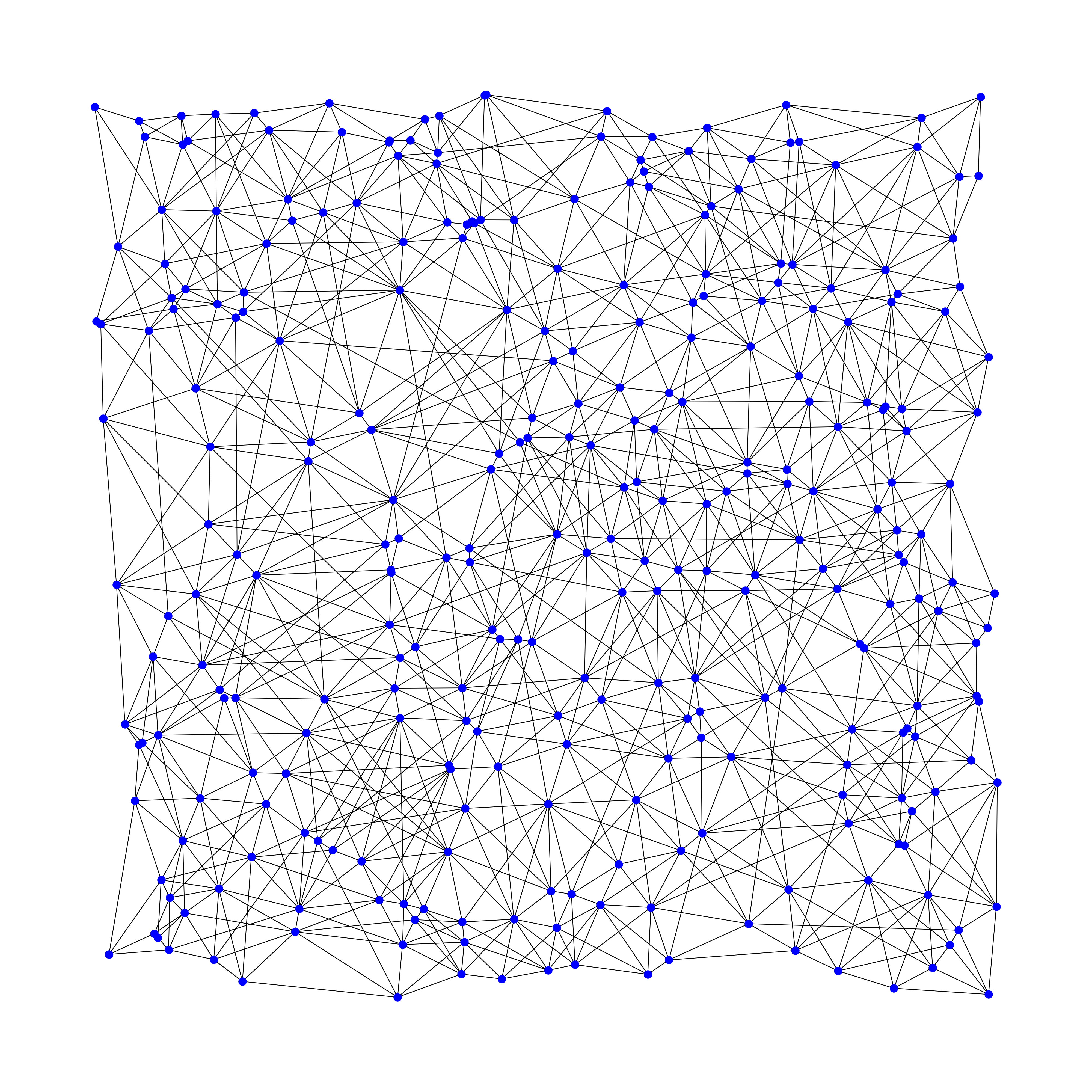
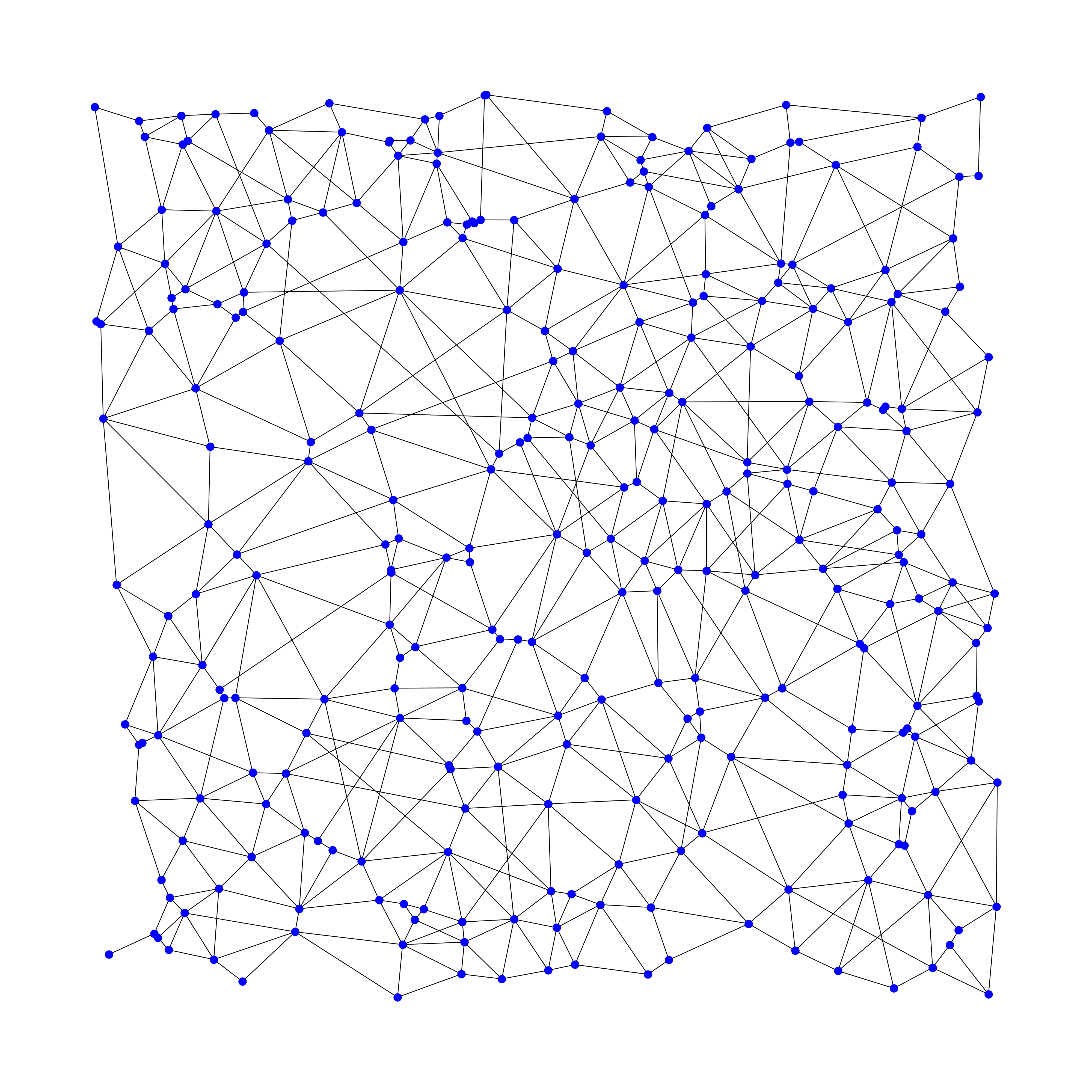
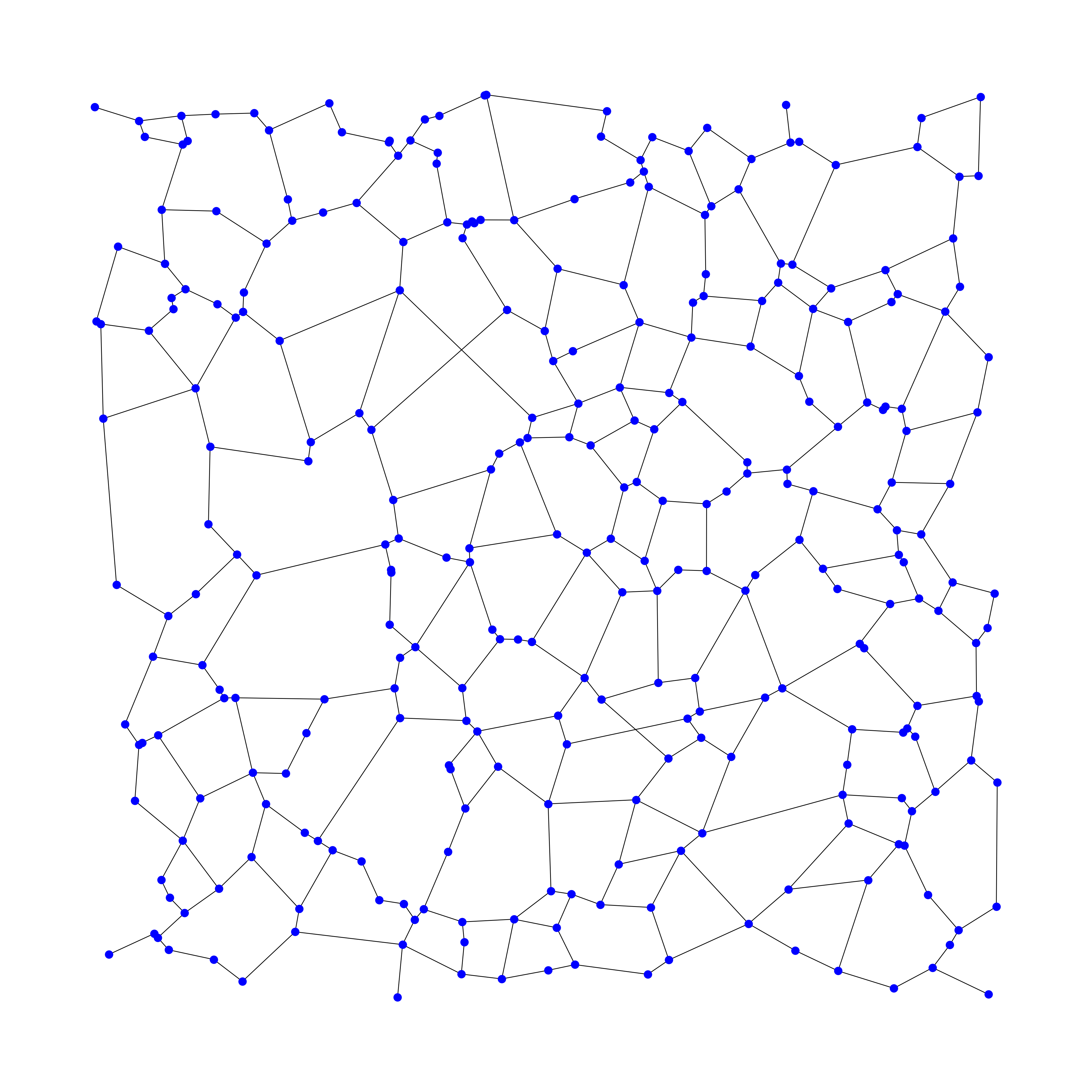
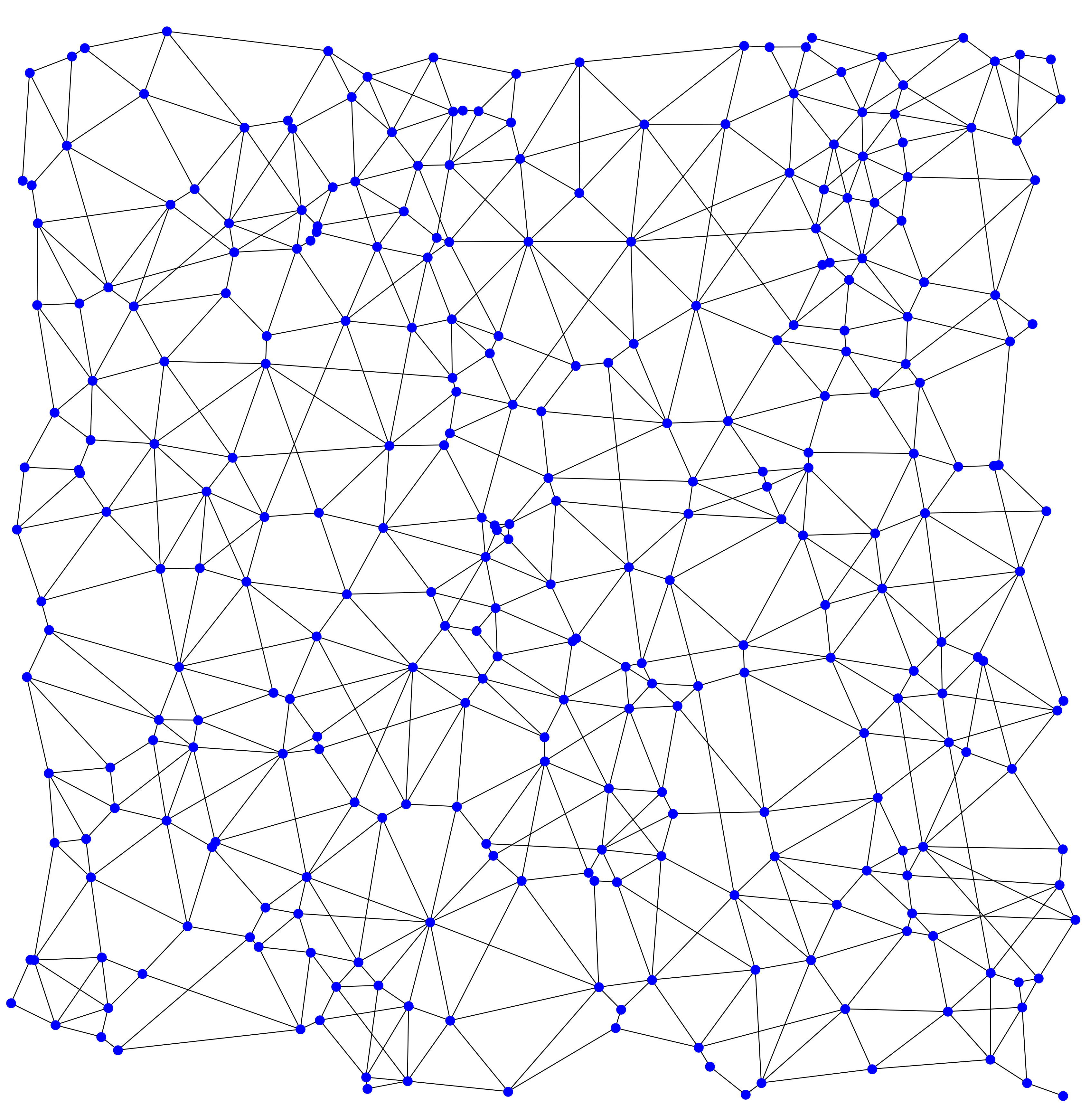
Introduced by Althöfer et al. [4] and also by Chandra et al. [16] more than years ago, the greedy spanner is a cornerstone in the study of geometric spanner networks, offering near-optimal guarantees in terms of sparsity and weight (also lightness) [10, 20, 21, 26, 32]. The greedy spanner is naively constructed by processing all pairs of points in order of increasing Euclidean distance and adding an edge between each pair if the current shortest path between them exceeds , where is the desired stretch factor. The algorithm, known as Path-Greedy in the literature, is a generalization of the textbook Kruskal’s algorithm. Refer to Figure 1 for greedy spanner examples.
|
 |
|---|---|
| (a) | (b) |
|
 |
| (a) | (b) |
A straightforward implementation of Path-Greedy runs in time since there are point pairs, and for every pair, computation of a shortest path takes time, as greedy spanners are linear-sized spanners. It also uses space to store and sort all point pairs, making it impractical for large point sets. A variant (still using extra space), named FG-Greedy, was introduced by Farshi and Gudmundsson [22], to speed up the algorithm by reducing the number of shortest-path calls. The idea was to memorize the shortest-path lengths obtained by previous single-source shortest-path calls using a matrix, allowing future calls to be avoided using simple lookups. Surprisingly, it was shown in [11] that FG-Greedy runs in time, although in experiments, it was found to be faster than Path-Greedy; refer to [22]. Das and Narasimhan made the first attempt to approximate greedy spanners in [19], wherein they designed the Approximate-Greedy algorithm that runs in time. See Table 1. Despite being theoretically novel, experimental studies [22, 32] on spanners found that Approximate-Greedy places substantially more edges compared to actual greedy spanners, rendering them impractical for real-world applications. Bose et al. [12] designed an -time algorithm to construct exact greedy spanners using space, an improvement over Path-Greedy. To see how frustrating quadratic space algorithms are in practice, consider . Storing all point pairs, at least of space is required, which is impractical. For this reason, we chose not to consider it in our experiments.
Alewijnse et al. [2] made the first significant attempt to construct greedy spanners on large point sets, marking a breakthrough. Their algorithm, referred to as WSPD-Greedy in [3], runs in time using only space, enabling the construction of geometric spanners on million-point instances for the first time. It avoids storing all pairwise distances by incrementally generating edge candidates via a well-separated pair decomposition (WSPD) [15, 25]. These candidates are processed in order of increasing distance using a priority queue, ensuring that only necessary edges are added while maintaining linear space complexity. The same authors devised an improved algorithm in [3], named Bucketing. It is a distribution-sensitive algorithm for constructing greedy spanners that exploits the geometric structure of point sets. They observed that most short edges can be determined locally, while long edges can be efficiently identified using the well-separated pair decomposition (WSPD). By leveraging a local characterization of -spanners, Bucketing achieves subquadratic expected time of on uniform distributions, making it the first such result for greedy spanners on any meaningful class of inputs. Bucketing was observed to be much faster than WSPD-Greedy; see [3] for experimental results. Abu-Affash et al. [1] designed the -greedy algorithm that retains the desirable properties of the Path-Greedy spanner, such as low degree, linear number of edges, and near-optimal weight, while significantly reducing the number of shortest path queries. The algorithm runs in time in the worst case, but achieves expected time on uniformly random point sets. The parameter controls the trade-off between construction time and similarity to the Path-Greedy spanner; setting yields an identical spanner. However, the space complexity is quadratic, making it impractical for large point sets. Therefore, we decided not to include it in our experiments.
Shariful et al. [32] recently observed that Bucketing is slow for large values of . For instance, when , , and the points are uniformly distributed inside a square, Bucketing took around five days to generate the spanner. So, they engineered a practical parallel algorithm Fast-Sparse-Spanner, that generated geometric graphs fast and had average degrees close to those of greedy spanners. Fast-Sparse-Spanner could generate a -spanner for the same above point set in just minutes, making it much faster than Bucketing in practice. They experimentally observed that Fast-Sparse-Spanner consistently generated -spanners across a wide variety of distributions and real-world point sets. To check for the -spanner property, they also devised an auxiliary practical stretch factor measurement algorithm, named Fast-Stretch-Factor, since Fast-Sparse-Spanner is not theoretically guaranteed to generate -spanners. However, the weights and degrees of the generated graphs are far from the actual greedy spanners owing to the presence of long WSPD spanner edges, which form a backbone of their spanners. Despite the average degree of the generated graphs being close to those generated by Bucketing (see Table 1), the degrees and lightness values substantially differed. For the point set used in Table 1, the degrees of graphs generated by Fast-Sparse-Spanner and Bucketing were 78 and 18, respectively, and the lightness values were 16.7196 and 11.0354, respectively.
Despite the progress made by Shariful et al. in [32], practical construction of spanners which closely resemble greedy spanners in terms of average degree, weight, and degree, especially for low -values (), remains an open problem. Note that Delaunay triangulations are -spanners [35] with edges that can be constructed in time (in practice, takes a few seconds even for millions of points). So, constructing -spanners with around or more is not considered challenging in practice.
What are doppelgängers of greedy spanners?
We introduce the notion of -doppelgänger. A -spanner on a point set is a -doppelgänger of the greedy spanner on , if its average degree and lightness do not exceed those of by more than additive constants and , respectively. Average degree and lightness are two central measures of spanner quality, and spanners with similar values for these metrics tend to be structurally similar. Thus, smaller values of and indicate better doppelgängers. Such doppelgängers are especially appealing to practitioners when they can be constructed significantly faster than the greedy spanner itself. The term “approximation” has not been used in this work intentionally, as the Approximate-Greedy [19] algorithm claims to generate spanners that are approximations of greedy spanners, but, in reality, they are structurally very different from the actual greedy spanners (also, see Table 1).
Our contribution.
Motivated by the lack of fast practical algorithm to generate -doppelgängers of greedy spanners for low values of and , we design and engineer -Greedy, a new spanner construction algorithm, based on -Graph. We found -Greedy to be considerably faster than our closest competitor Bucketing, and always produced high quality doppelgängers in our experiments. In our experiments, both and never exceeded . To our knowledge, no other known algorithm can achieve this while being fast and scalable in practice. See Figure 2 for a visual comparison between -Greedy and Bucketing.
We use the -Graph as a seed spanner since it can be constructed fast in time and, as seen in Table 1, excluding Fast-Sparse-Spanner (not guaranteed to produce -spanners), -Graphs have the lowest average degree and thus the lowest number of edges. We consider its edges by length and place them greedily, akin to Path-Greedy. Finally, we find point pairs that do not have -paths between them using a quad tree-based approach. For every such point pair, we establish a -path by placing edges carefully. Our algorithm can leverage multiple cores for speedup.
-Greedy is designed as an engineering solution to a long-standing practical bottleneck in geometric spanner construction rather than as a theoretical breakthrough. While its worst-case complexity is , the algorithm consistently exhibits near-quadratic scaling in practice and uses linear space, enabling it to handle million-point datasets efficiently. It leverages heuristic path checks and shortcut caching to achieve massive speedups, up to x faster than Bucketing, while producing spanners that are structurally almost indistinguishable from true greedy spanners in terms of degree and lightness. The focus of -Greedy is on simplicity, scalability, and reproducibility for real-world geometric networks, not on improving asymptotic bounds.

Preliminaries.
A region quad tree is a hierarchical spatial data structure that recursively partitions a two-dimensional region into four congruent quadrants until each subregion is homogeneous or its size falls below a specified threshold , the maximum leaf size. The root node represents the entire region, and each internal node corresponds to a square subdivided into four child quadrants. A -Graph [28] is a geometric spanner constructed by dividing the plane around each point into equal-angle cones and connecting the point to the vertex in each cone that minimizes the distance projected onto the cone’s bisector. The constructed geometric graph is a -spanner if , where . -Graph can be constructed in time [28].
2 Description of -Greedy
This section presents the steps of the -Greedy algorithm in order. Let denote the output spanner constructed on the input point set of size . Initially, is an empty graph.
Step 1. Construct a minimum spanning tree on by running Prim’s algorithm on the edges of a Delaunay triangulation of . Place the edges of in . Since the Path-Greedy algorithm will place such edges, irrespective of the value of , we can compute such edges quickly and place them in advance to avoid shortest-path calls.
Step 2. Refer to Algorithm 1. We construct a -Graph -spanner on . Let be the set of edges in . Sort the edges in in non-decreasing order of length. Then, process them greedily, following the spirit of the Path-Greedy algorithm: For each edge , if no -path exists between and in , insert into ; otherwise, skip the edge.
To check for an -path between , we first invoke an heuristic algorithm called Greedy-Path, which avoids the use of a priority queue, unlike standard shortest-path algorithms such as or Dijkstra. This heuristic is inspired by the work [32]. We make use of shortcuts, as described next, to speed it up. The Greedy-Path performs a walk from to in , aiming to discover a path greedily, whose total length does not exceed . At each step, it evaluates candidate next hops drawn from two sources: (i) precomputed -paths obtained by previous Greedy-Path and calls, stored in shortcuts, as described next (also see Algorithm 1), and (ii) the actual graph neighbors of the current vertex. For every candidate, it computes a simple score - the current path length greedily constructed so far plus the edge (or shortcut) cost to that candidate, plus its straight-line (Euclidean) distance to as an optimistic estimate of continuing via that vertex. It then moves to the candidate with the lowest score, marking visited choices to avoid cycling, and it stops immediately if is reached. If the accumulated path length exceeds the stretch upper bound, the heuristic declares failure; otherwise, it returns the achieved -path.
If Greedy-Path finds a -path, we store it as a shortcut (with its weight) in a structure shortcuts, similar to an adjacency list, to accelerate future queries. If Greedy-Path fails, we fall back to the popular algorithm. If also fails, we insert into ; otherwise, we store the discovered -path in shortcuts for future use. Note that to maintain the linear size of shortcuts, it is not updated in Steps 3, 4, and 5 of our algorithm.
Step 3. Construct a region quad tree on such that the number of points contained inside every leaf is no more than a fixed constant . In our experiments, we found that was sufficient. For every leaf , ensure that a -path exists in , between all point pairs in , where is a subgraph of , induced by the points in . This is achieved by running Dijkstra from every point in . Let be the set of point pairs from all the leaves that do not have -paths in . Sort , and place edges greedily. Akin to Step 2, we first use Greedy-Path, followed by , if necessary. While adding edges greedily, we check for the existence of -paths by considering rather than .
Step 4. Let be an empty set of edges. For every leaf pair , ensure -paths in between all point pairs . If a pair is found not to have a -path in , place the edge in and add the same to . Akin to Step 2, we use Greedy-Path followed by . For a given leaf pair , the -paths (bridges connecting distant point pairs) found are temporarily stored in a list . Since , . Its use is based on the observation that points from faraway tend to share -paths. Consequently, we save -path computations by first searching for a valid bridge in , where such that . If , terminate this step early and go to Step 5. Since every leaf pair is considered independently, a super-linear number of edges could be placed in this step. The following step is a fail-safe step to ensure linearity.
Step 5. If , delete all the edges in from . For every leaf pair , find all point pairs , that do not have -path in . Similar to Step 4, Greedy-Path is used first, followed by (if the former fails to find a -path). Let be the set of all such pairs. Sort , and place edges greedily in .
Next, we show in Theorem 1 that is a sparse -spanner on .
Theorem 1.
For any fixed , is a -spanner with edges.
Proof.
The algorithm begins by inserting the edges of a minimum spanning tree into . Since is connected and contains exactly edges, is connected after Step 1. In Step 2, we place edges since the size of is , for fixed . Step 3 introduces edges as is a constant. We insert at most edges within each leaf of , and since has leaves, the total number of edges added is . If Step 4 places at most edges, then clearly, has edges.
Now, let us assume that the number of edges placed in Step 4 exceeds (possibly ). In what follows, we argue that in such a scenario, Step 5 places edges, thereby proving our sparsity claim for .
Let be any vertex of . We claim that the number of edges placed in Step 5, that are incident on , is at most , such that satisfies the inequality, . Assume, for contradiction, that two edges and are added in Step 5, where , and both lie in the same cone (with angle ). Since the edge was processed first, it is already in the graph when is considered. For the edge to be prevented from insertion into , the path going through must provide a -path in : .
We analyze the worst-case geometric configuration where and are located on the two distinct bounding rays of the cone, maximizing the distance for angle . Refer to Figure 3. An upper bound on can be given by the distance projected onto the ray containing plus the stretch factor applied to the orthogonal component: . To prevent the insertion of the edge in , this upper bound must be less than or equal to . Thus, . Dividing both sides by , we obtain the necessary angular constraint: . We conclude that there are at most edges placed that are incident on in . For fixed , . Hence, Step 5 places edges.
The -spanner property of follows directly from Steps 3, 4, 5. In Step 3, we ensure -paths between all point pairs inside every leaf of . In Steps 4 and 5, we ensure -paths between all point pairs where they belong to distinct leaves of .
Thus, is a -spanner with edges.
Time complexity.
Step 1 runs in time as Delaunay triangulations can be constructed in time (via Voronoi diagram) having at most edges and Prim’s algorithm on edges runs to completion in time. Next, the construction of the -Graph takes time [28]. Also, . For every pair , verifying the existence of a -path between takes time in the worst-case due to the use of Greedy-Path that runs in time followed by that runs in time in the worst-case. For pairs in , the total time taken is . So, Step 2 runs in time. In Step 3, constructing takes time in the worst case. The remaining part of this step takes time since the size of every leaf is at most . For every leaf of , there are point pairs not having -paths. For leaves, there are such point pairs. Detecting such pairs takes time since the size of every is . Finally, Steps 4 and 5 each take time since there are non-empty leaf pairs of and for every such pair we spend time for detecting -paths between point pairs. Thus, the overall worst-case time complexity of -Greedy is .
Remark on high time complexity.
Although -Greedy has a worst-case complexity of , this bound is highly pessimistic. It assumes that Steps 4 and 5 spend time for every leaf-pair due to calls. In practice, this scenario rarely occurs. First, is seldom invoked because Greedy-Path successfully finds -paths in most cases. When Greedy-Path is used, its directional exploration visits only a small fraction of vertices before terminating, making each check extremely fast. Second, when a long -path is discovered between two distant leaves , it typically suffices for almost all point pairs , greatly reducing the number of subsequent calls. Combined with bridge reuse and shortcut caching, these effects make Steps 4 and 5 far cheaper than the worst-case analysis suggests. As a result, -Greedy exhibits near-quadratic scaling in practice, as confirmed by our experiments on diverse synthetic and real-world datasets in Section 3.
Space complexity.
The extra space needed by Prim’s algorithm and the Delaunay triangulation construction in Step 1 is . Constructing and storing takes space. Greedy-Path and takes extra space. The data structure shortcuts uses space since, in the worst case, it can contain one -path per edge in . The quad tree in Step 4 uses space, where is its height. So, the extra space required by -Greedy is , since . Thus, -Greedy behaves like a linear-space algorithm in practice, making it possible to generate spanners on point sets where is as large as .
3 Experiments
Setup.
The algorithms were implemented in C++23 using GCC 13 and the CGAL 6.1 library [33]. The boost library was used for common algorithms and data structures. Refer to Table 2. All experiments were conducted on a desktop running Ubuntu Linux 24.04 LTS, equipped with an Intel Core i9-12900K processor and 32 GB of RAM. From CGAL, we employed the CGAL::Exact_predicates_inexact_constructions kernel. The entire codebase was compiled with the O3 optimization flag to maximize performance.
![[Uncaptioned image]](library.png)
Synthetic point set distributions.
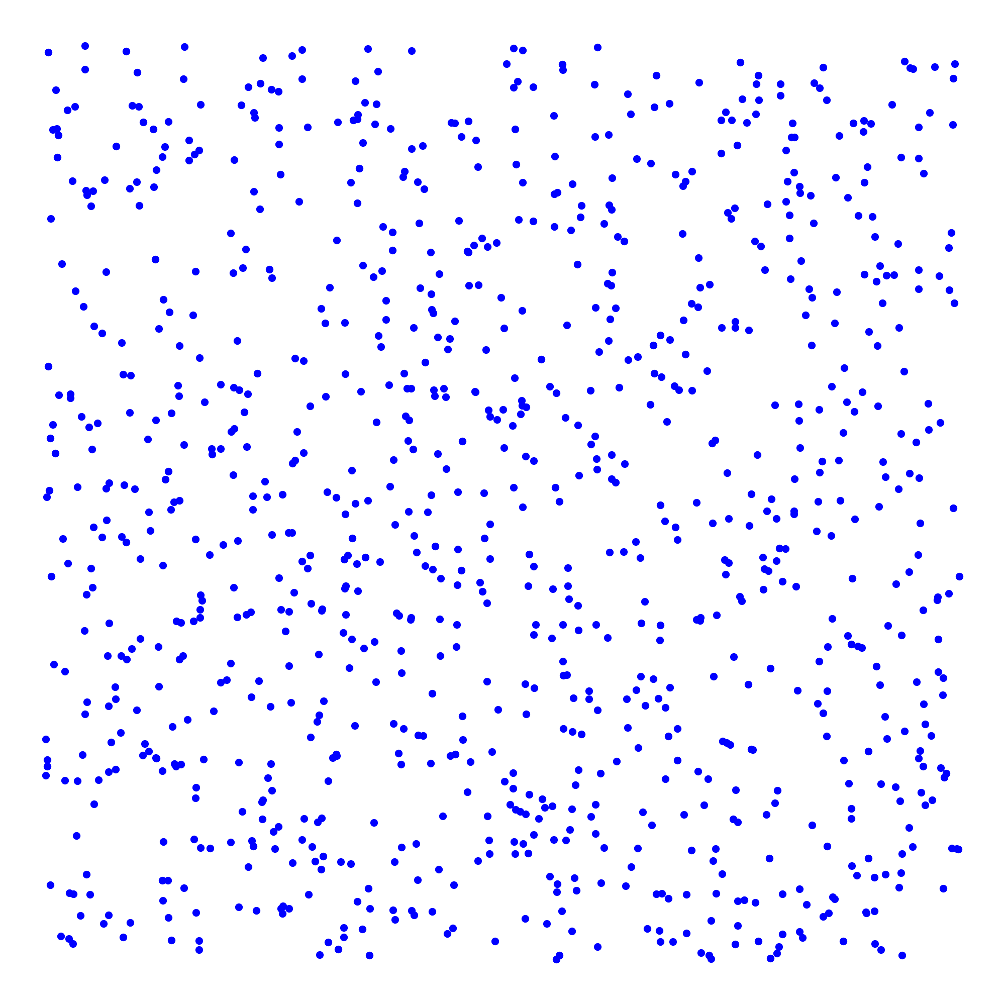
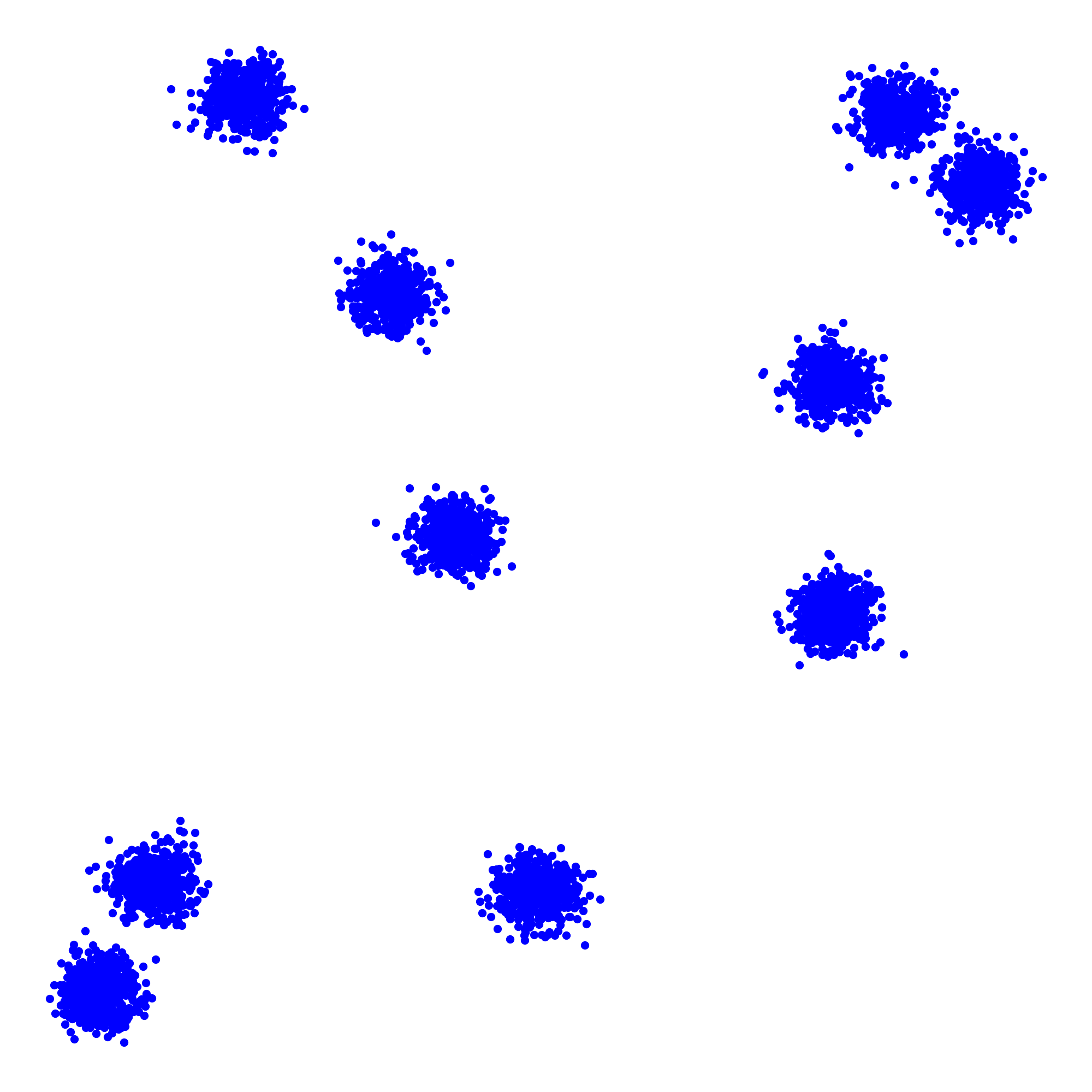
We used five point set distributions to generate random point sets. These distributions were adopted from previous experimental studies [6, 9, 23, 29, 32]. They are named uni-square, normal-clustered, grid-random, annulus, and spokes. Refer to Figure 4 for an illustration.
The uni-square distribution generates points uniformly within a square region using CGAL::Random_points_in_square_2. It is the most common distribution used in geometry experiments. The normal-clustered distribution places points in randomly positioned clusters, where each cluster follows a normal distribution with a fixed mean and standard deviation. Since the clusters are separated by long distances, shortest-path calls tend to take a long time. Hence, we chose it for our experiments. The grid-random distribution scatters points across a non-contiguous grid within a scaled square, with integer coordinates chosen uniformly at random. This distribution is important because of the collinearity present throughout its point sets. In Figure 4, although it resembles uni-square, the coordinates of the points are restricted to integers. The annulus distribution positions points inside a ring-shaped region defined by inner and outer radii, using real-valued uniform sampling. This distribution is important because of the large hole present inside the point sets. The spokes distribution organizes points along five radial spokes emanating from a central point. The vast separation between the collinear spokes is useful for testing spanner algorithms. For each of the above distributions, we considered eight values of , selected from the set . For every value of , we sampled five point sets.
Real-world point sets.
Real-world point sets are essential because they reflect the actual spatial distributions and irregularities encountered in practical applications. Synthetic datasets, while useful for controlled benchmarking, often assume idealized conditions, such as uniform distributions, perfect clustering, or simplified geometries, that rarely occur in reality. Real-world data introduces challenges, such as uneven point density and non-uniform patterns, which may significantly influence spanner construction time and structural properties. Testing on real-world datasets ensures that algorithms are robust, scalable, and effective under realistic conditions. In our experiments, we used six real-world datasets, as described next.
| Dataset | burma | birch3 | monalisa | KDDCU2D | usa | europe |
|---|---|---|---|---|---|---|
| 33,708 | 99,999 | 100,000 | 104,297 | 115,475 | 168,435 |
 |
 |
| (a) uni-square | (b) normal-clustered |
 |
 |
| (c) grid-random | (d) annulus |
 |
| (e) spokes |
The burma dataset consists of 33,708 points representing cities across Burma. The birch3 dataset contains 99,999 points arranged in random clusters scattered throughout the plane. The monalisa dataset is a 100,000-city TSP instance depicting a continuous-line drawing of the Mona Lisa. The KDDCU2D dataset includes 104,297 points corresponding to the first two dimensions of a protein dataset. The usa dataset represents a large-scale TSP instance with 115,475 cities covering nearly all towns, villages, and cities in the United States. Finally, the europe dataset comprises 168,435 points encoding differential coordinates of the European map. Refer to Table 3 for a summary.
Metrics and comparisons.
Next, we compare -Greedy with Bucketing using runtime, degree , average degree (), and lightness as metrics.
-
1.
Runtime. When constructing spanners on large point sets, runtime becomes a critical concern. Guaranteeing a -path between every pair of points remains a significant challenge. For synthetic point sets, the maximum speedup was observed when (the smallest value used in our experiments) and . Refer to Figures 5, 6, 7, 8 and 9. For every value of , the average runtime of five runs is reported. The corresponding speedups were , , , , and for uni-square, normal-clustered, grid-random, annulus, and spokes respectively. For real-world point sets (Table 4), the highest speedup of occurred for the europe dataset when . As discussed next, -Greedy achieved these speedups while maintaining low values of and , ensuring high-quality -doppelgängers. We also observed that Bucketing could match the speed of -Greedy when ; however, in that case, -Greedy can be easily accelerated further by using additional threads.

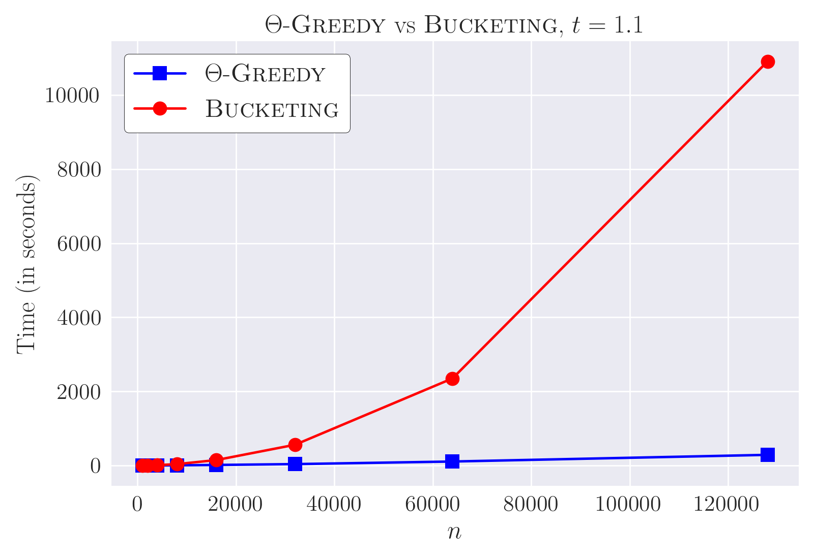
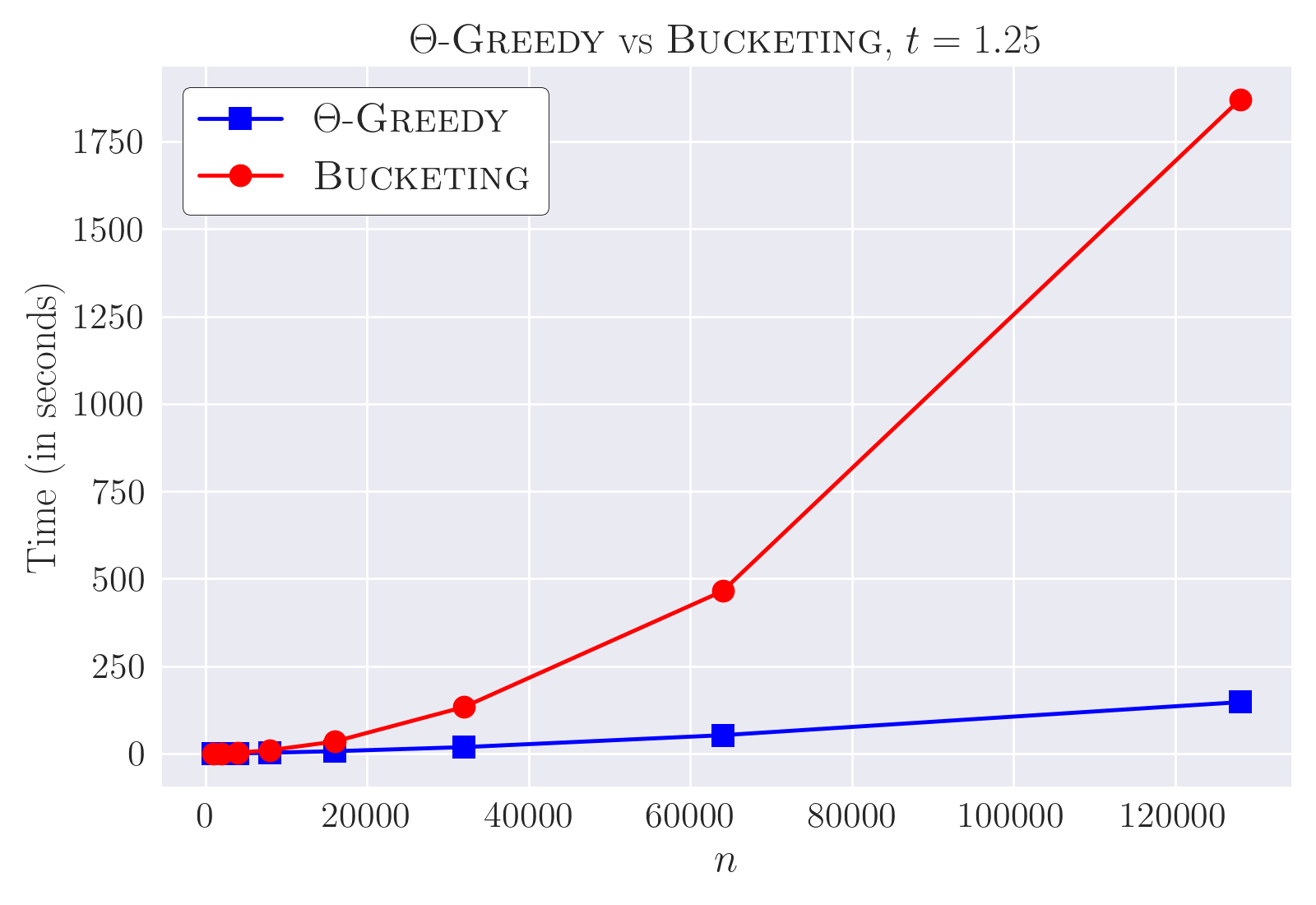
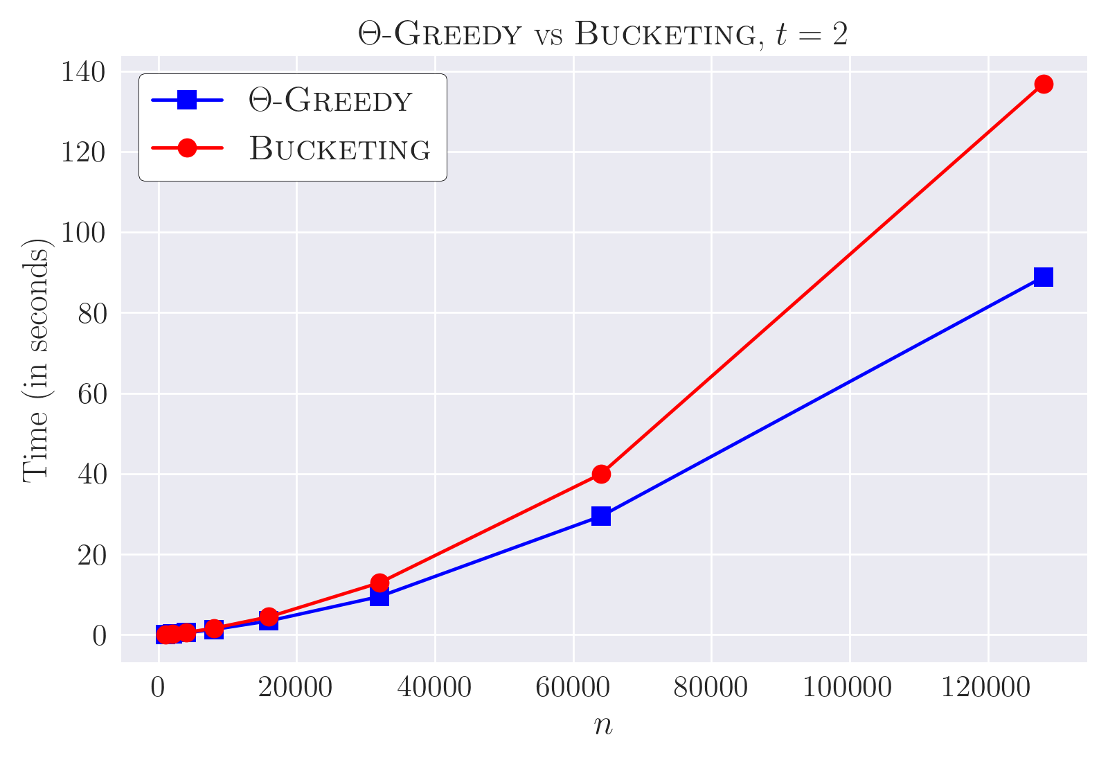
Figure 5: -Greedy vs Bucketing; runtime comparison for the uni-square distribution. 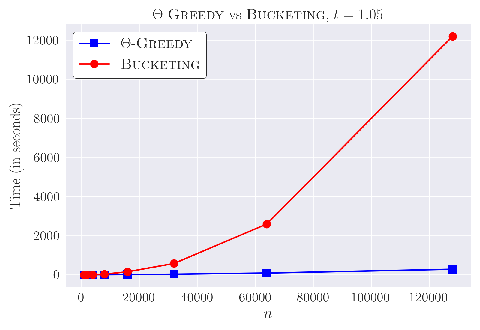

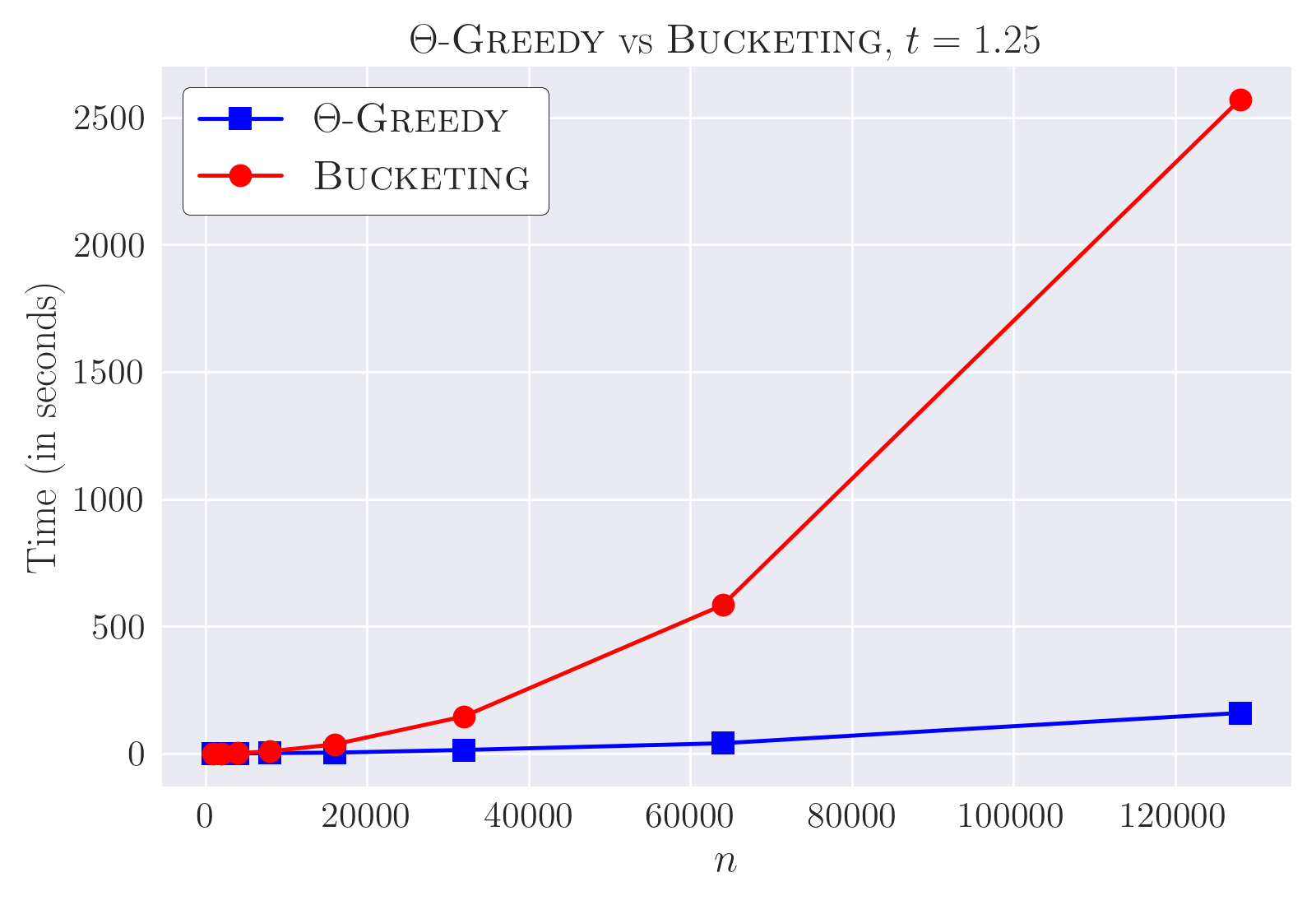
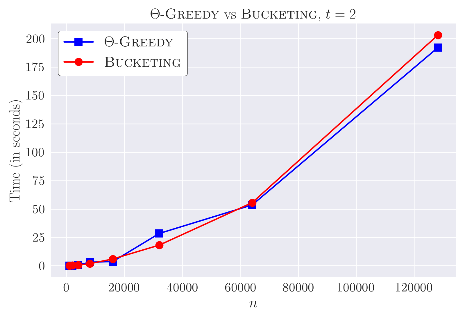
Figure 6: -Greedy vs Bucketing; runtime comparison for the normal-clustered distribution. 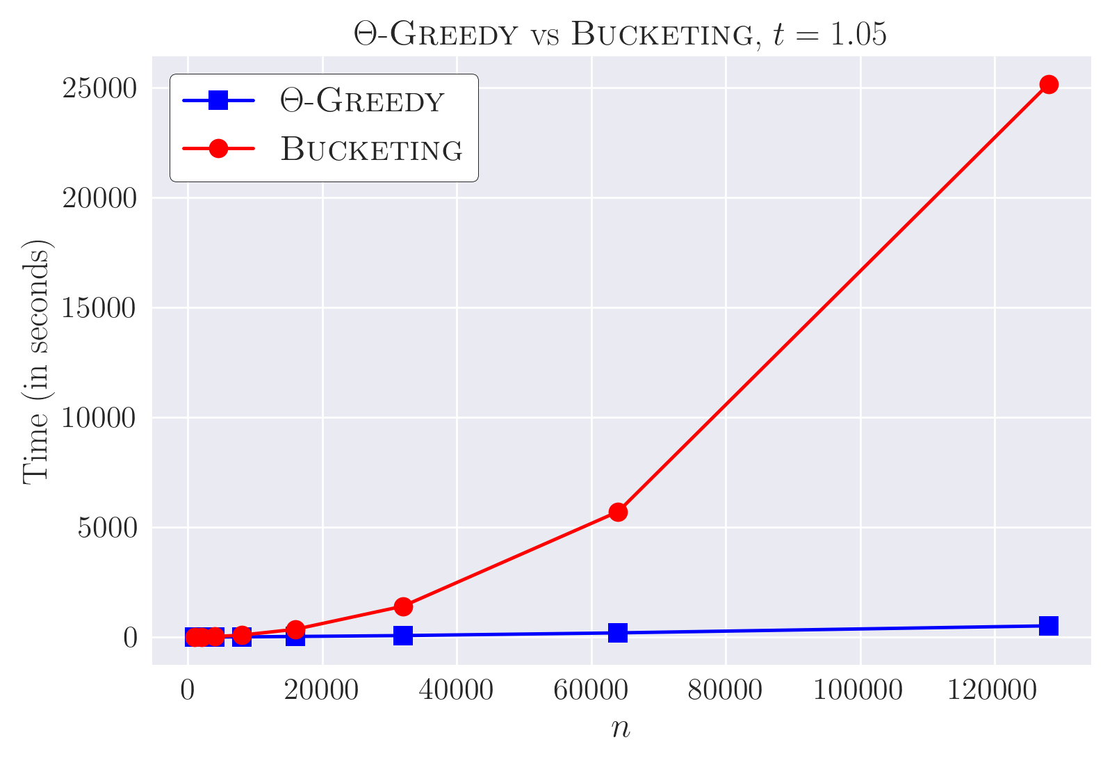
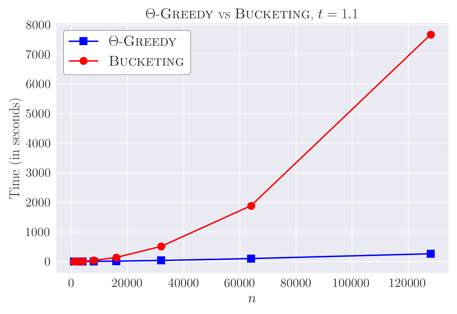


Figure 7: -Greedy vs Bucketing; runtime comparison for the grid-random distribution. 

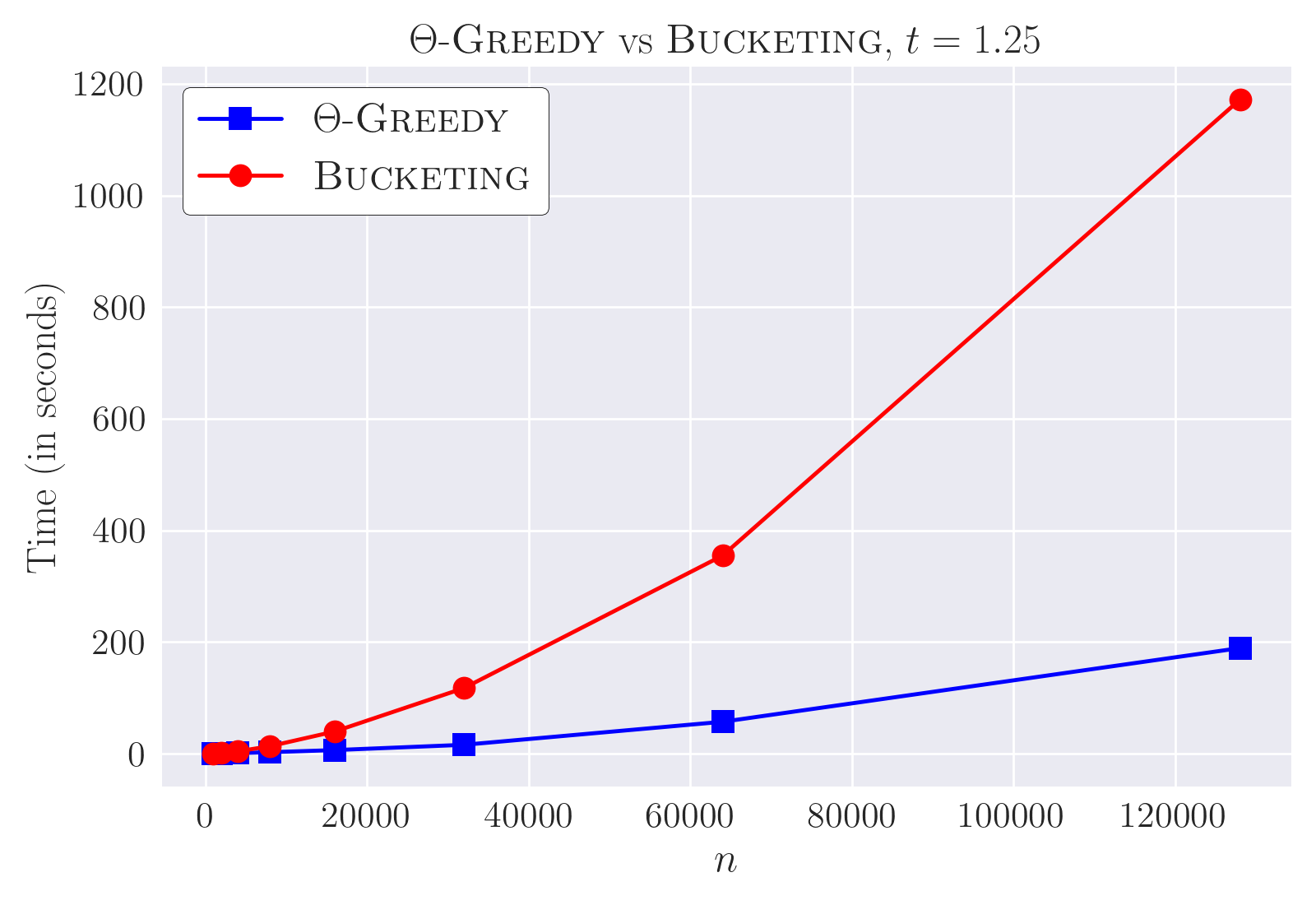
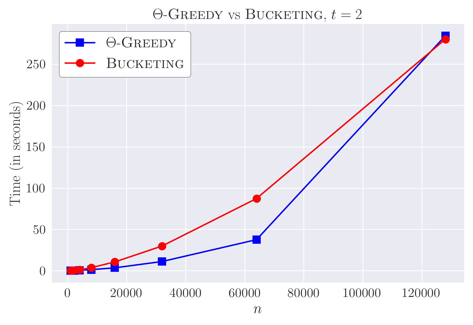
Figure 8: -Greedy vs Bucketing; runtime comparison for the annulus distribution. 
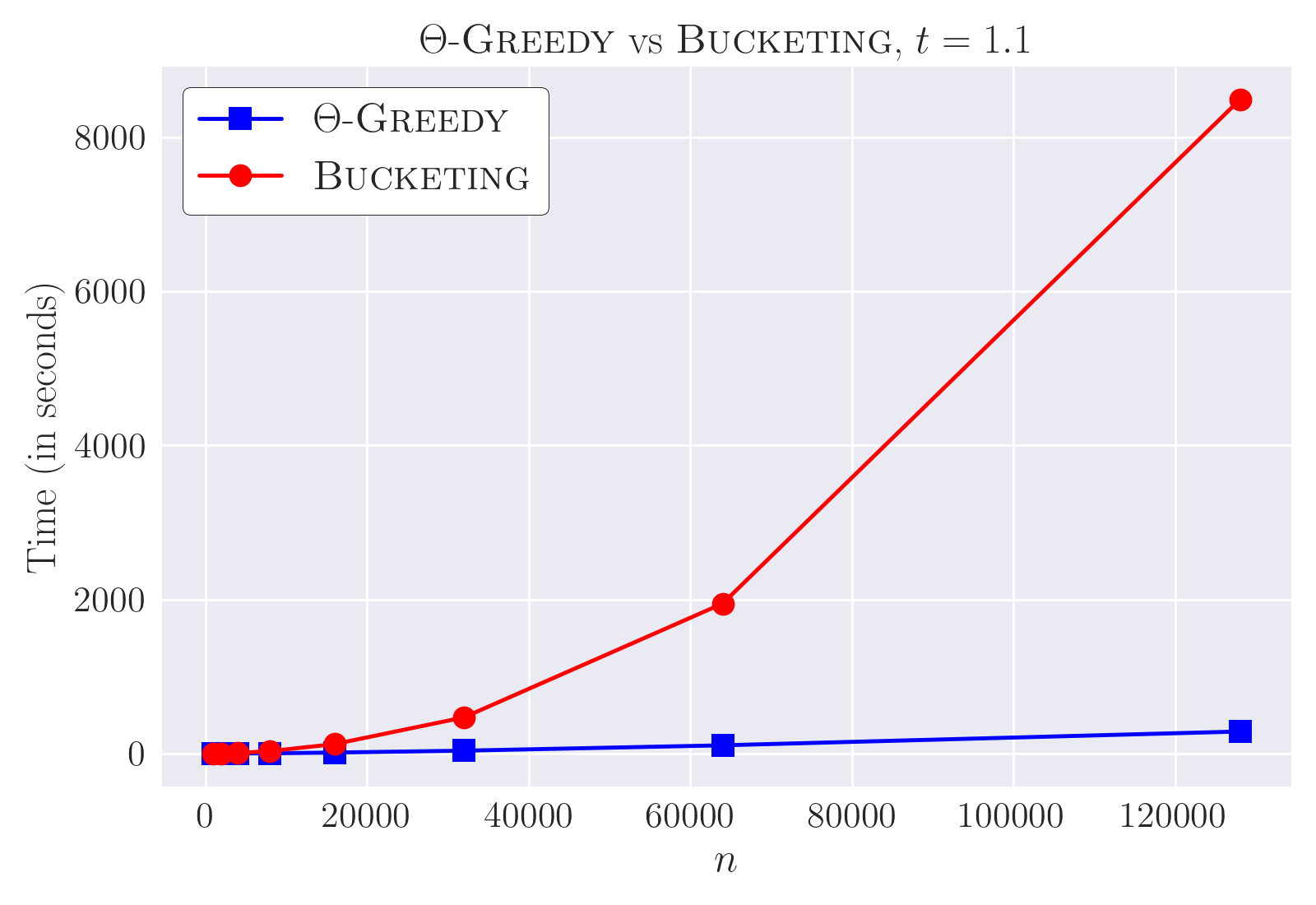
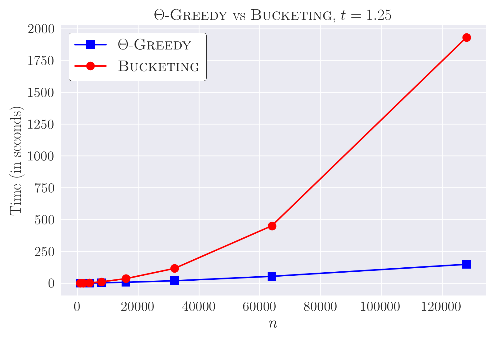

Figure 9: -Greedy vs Bucketing; runtime comparison for the spokes distribution. For point sets of size , -Greedy completed within a few hours (Table 6) using just one thread. Shariful et al. [32] reported that Bucketing requires about five days for the uni-square distribution, whereas -Greedy finished in roughly two hours, corroborating its remarkable efficiency. For other distributions, -Greedy consistently performed well, completing within a few hours. The slowest case was the normal-clustered point set, which took about four hours due to the presence of long -paths in the final spanner, causing Greedy-Path and to run slower.
Table 4: Runtime (in minutes), degree (), average degree (), and lightness comparisons are shown for the real-world point sets. stands for threads, respectively. ![[Uncaptioned image]](realworld.png)
-
2.
Degree and average degree. Degree matters for load balancing and hardware constraints. For instance, in computer networks, a node with too many connections consumes more energy and bandwidth. Consequently, a low degree is desired. The average degree metric reflects the overall sparsity and efficiency of a network. A low average degree means fewer edges per vertex, reducing cost and complexity while maintaining connectivity.
Table 5: The maximum observed values for and with respect to the spanners produced by Bucketing. uni-square normal-clustered grid-random annulus spokes real-world 0.0000 0.0000 0.0020 0.0010 0.0005 0.0000 0.0000 0.0111 0.0056 0.0875 0.0030 0.0600 According to the definition of -doppelgängers, introduced in Section 1, lower values for and are desired. We found that for both synthetic and real-world point sets, the maximum value of did not exceed , when all four values of were considered; refer to Table 5. This shows that -Greedy is capable of producing greedy-like sparse spanners. To our knowledge, no other practical algorithm matches this performance.
Regarding the actual difference in degrees, we observe that it is always for the real-world point sets (Table 4) and at most for the synthetic point sets. The maximum value of 4 occurs for the annulus instances, whereas for uni-square the difference remains 0.
-
3.
Lightness. It is crucial because it controls the total cost of connectivity. In real-world networks, such as transportation systems, wireless sensor deployments, or fiber-optic layouts, lower lightness means the network uses short edges while still guaranteeing good connectivity. This translates to lower construction costs, reduced energy consumption, and easier maintenance, making spanners both efficient and practical. As with the average degree, we found that the lightness of -Greedy spanners was very close to that of Bucketing spanners. Refer to Table 5. For the synthetic point sets, the maximum value of was 0.0875, achieved for the annulus distribution. For the real-world point sets, it was , achieved for the burma dataset, when ; see Table 4.
Multithreaded performance.
We now describe how -Greedy is parallelized using OpenMP. The construction of the -Graph is naturally parallelizable, since the edges generated for each point are independent. In Step 2, we process edges from in batches of size , where is the number of threads. For each batch, we run instances of Greedy-Path in parallel. Let denote the number of edges in the batch whose endpoints are not connected by a -path, as determined by Greedy-Path. For these edges, is then executed sequentially to find -paths and insert edges in whenever required. Since Greedy-Path successfully finds -paths in most cases where such paths exist in , calls to are comparatively infrequent. Detection of violating point pairs (i.e., pairs lacking -paths) in the leaf nodes is independent in Step 3 and therefore parallelizable. In Steps 4 and 5, all leaf pairs , where is fixed, are also processed in parallel.
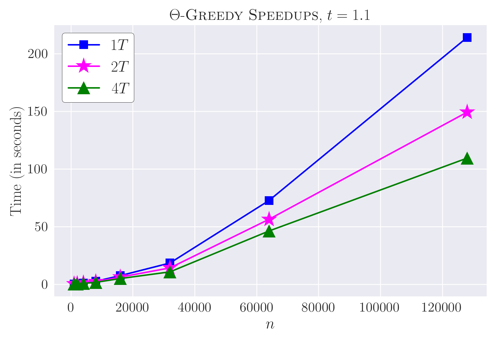
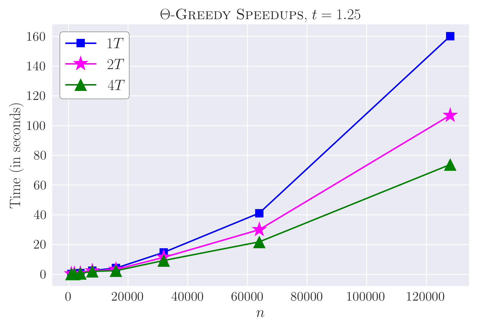
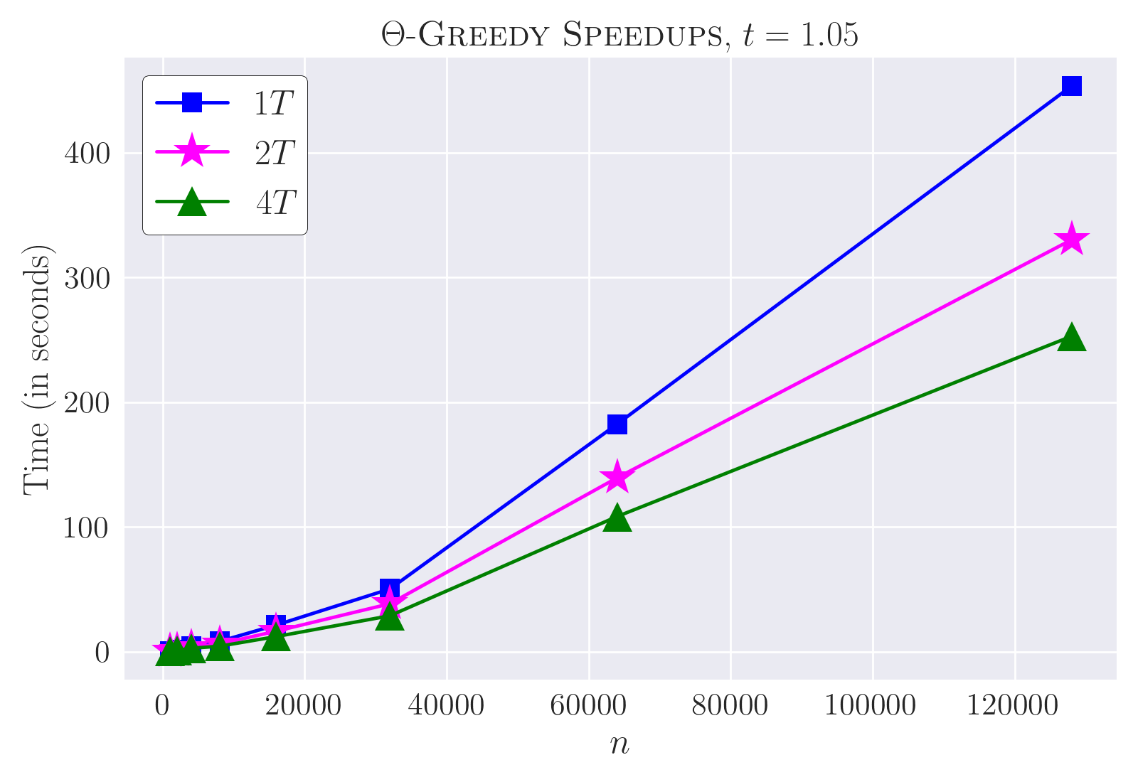
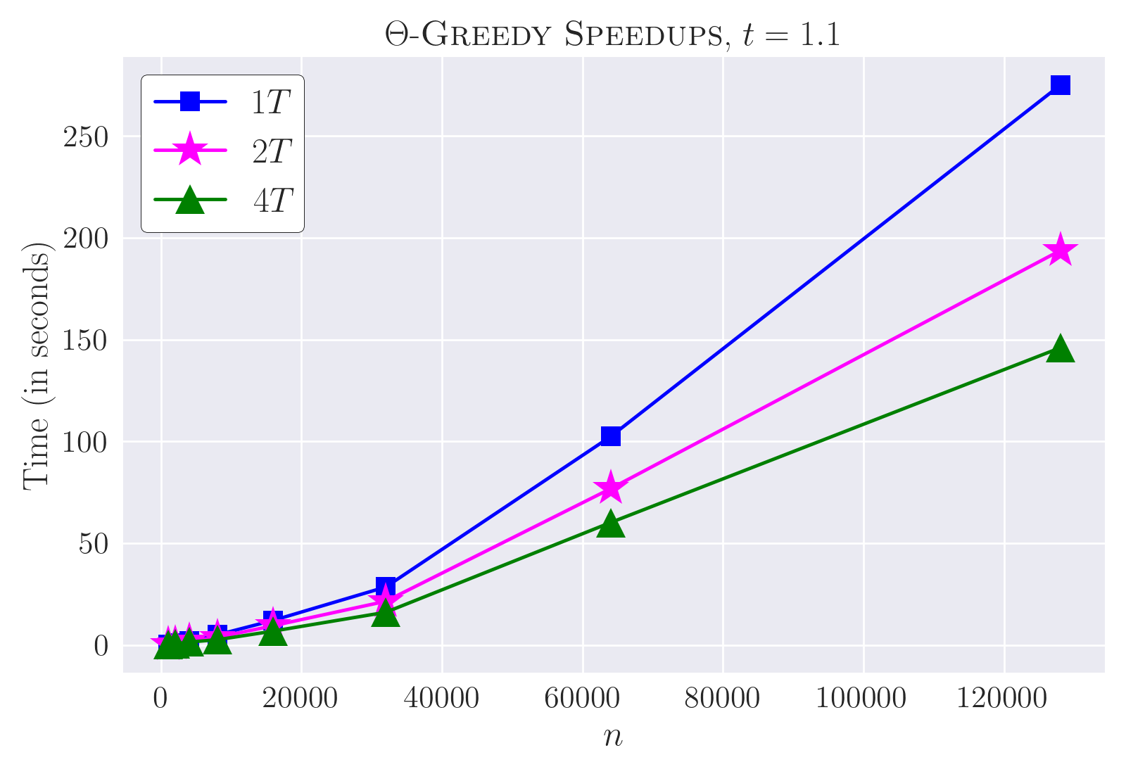
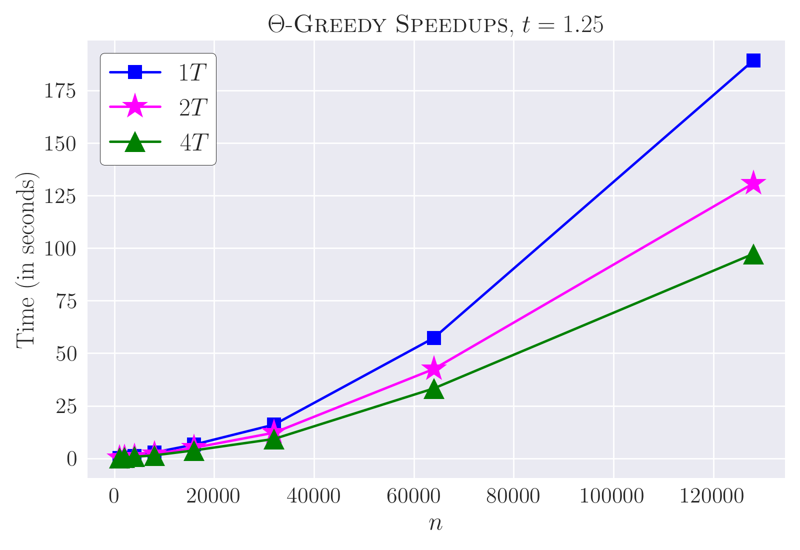
The above approach yielded speedups proportional to , making -Greedy scalable for large point sets. Refer to Figures 10, 11, 12, 13, 14 and Tables 4 and 6. We observed consistent speedups across all values of used in our experiments.





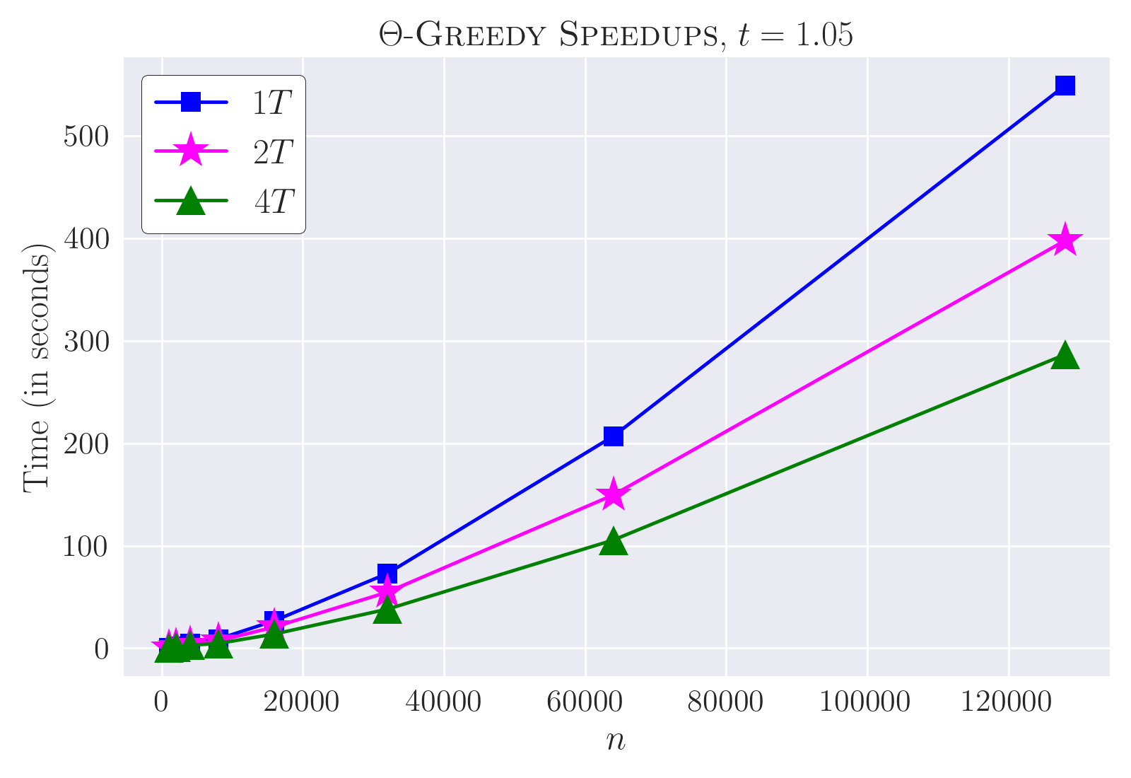

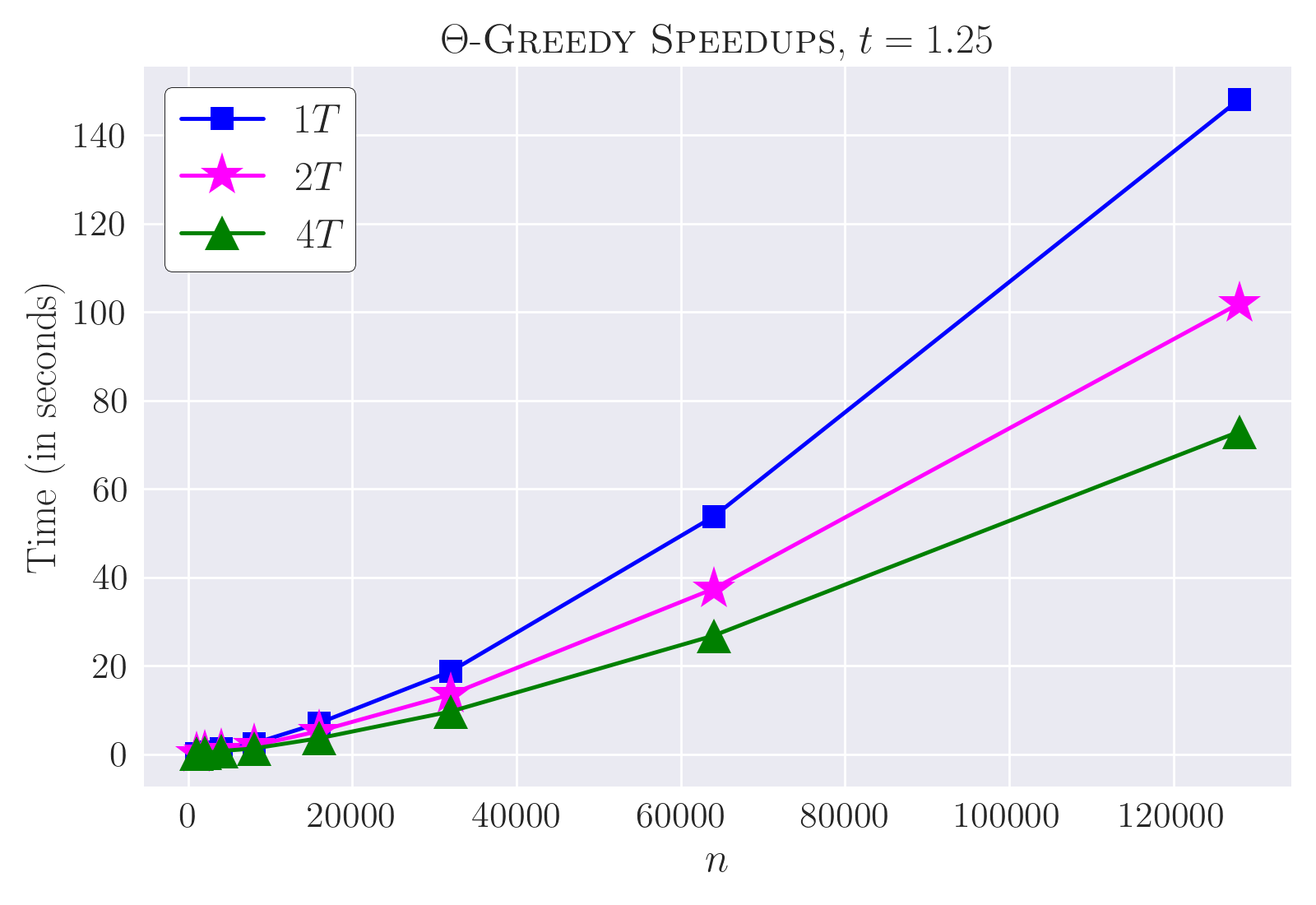
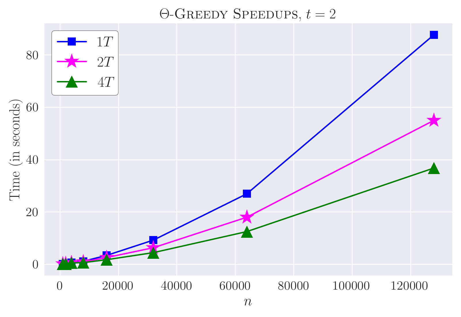
Comparison with Fast-Sparse-Spanner.
Since Fast-Sparse-Spanner [32] was the only previously known practical algorithm for constructing spanners on large point sets, it is natural to compare our algorithm against it. Since one run of Bucketing on a million points takes several days (roughly 5 days for uni-square), it is impractical for comparison purposes. However, the trends show that -Greedy spanners are still competitive with Bucketing spanners even for massive point sets. For instance, for the uni-square point set, we found the average degree to be , which is roughly the same as that of the -element point set used in Section 1 (the reported value for Bucketing is ).
See Table 6, where we set and . The spanners produced by -Greedy have significantly lower degrees than those generated by Fast-Sparse-Spanner, indicating that the resulting spanners differ substantially. The biggest differences were achieved for the uni-square and grid-random point sets. Interestingly, for the -element uni-square point sets, the maximum degree was at most 19 for ; the same value was observed even when . This demonstrates that our algorithm preserves greedy-like degree behavior even for massive point sets.
Although the differences in average degree are modest, the number of edges inserted by Fast-Sparse-Spanner is noticeably higher. For example, on the uni-square point set, Fast-Sparse-Spanner added roughly 455,000 more edges than -Greedy. Moreover, the Fast-Sparse-Spanner spanners were substantially heavier than the -Greedy spanners. This is primarily due to the long WSPD-spanner edges that Fast-Sparse-Spanner employs as a backbone. Taken together, these observations clearly demonstrate the superiority of -Greedy over Fast-Sparse-Spanner.
| , | uni-square | normal-clustered | grid-random | annulus | spokes |
|---|---|---|---|---|---|
| -Greedy Runtime | 123.69 | 239.32 | 124.44 | 188.76 | 125.86 |
| -Greedy Runtime | 89.57 | 160.6 | 88.22 | 125.61 | 86.73 |
| -Greedy Runtime | 69.31 | 108.47 | 70.51 | 88.3 | 65.02 |
| -Greedy | 19 | 19 | 19 | 19 | 18 |
| Fast-Sparse-Spanner | 1002 | 625 | 1003 | 573 | 972 |
| -Greedy | 9.1 | 8.84 | 9.1 | 9.07 | 9.1 |
| Fast-Sparse-Spanner | 9.97 | 9.15 | 9.84 | 9.6 | 9.88 |
| -Greedy Lightness | 11.08 | 9.88 | 11.07 | 11.67 | 11.07 |
| Fast-Sparse-Spanner Lightness | 238.62 | 3164.69 | 236.36 | 164.9 | 213.22 |
Finally, the lightness of the -Greedy spanners were significantly lower. See Table 6. The largest disparity occurred for the normal-clustered point set, where the lightness of the Fast-Sparse-Spanner graph was approximately times greater than that of the -Greedy spanner.
We observe that Fast-Sparse-Spanner is faster than ours in practice. In particular, for uni-square, normal-clustered, grid-random, annulus, and spokes, the time taken by the algorithm was roughly , , , , and minutes, respectively, on a system comparable to ours using one thread. Fast-Sparse-Spanner, ran fastest on the normal-clustered point set due to the long WSPD-edges connecting distant clusters, owing to which -path verifications terminated much faster compared to ours. In our case, the opposite happened, and we observed that -Greedy was slowest on the same point set and took almost hours to finish due to the presence of much longer -paths between distant clusters. With the increase in the number of threads (), -Greedy could accelerate in all five cases.
4 Conclusions
We introduced -Greedy, a practical parallel algorithm for constructing doppelgängers of greedy geometric spanners that are structurally and metrically almost indistinguishable from the actual greedy spanners. Thus, -Greedy spanners serve as practical and reliable alternatives to true greedy spanners. In our experiments, we found that -Greedy consistently achieved almost-greedy sparsity, lightness, and degree distribution while scaling to million-point instances with linear space and significant speedups over Bucketing, the fastest known greedy spanner algorithm. Our results close a long-standing gap between theoretical optimality and practical feasibility for low stretch factors, offering the first engineered solution that combines simplicity, efficiency, accuracy, and scalability for large real-world geometric networks.
An exciting avenue for future work is reducing the worst-case time complexity of -Greedy without sacrificing its ability to produce doppelgängers. Exploring distribution-sensitive optimizations and GPU acceleration could further broaden its applicability. Additionally, extending these ideas to higher dimensions remains a compelling open problem.
References
- [1] A Karim Abu-Affash, Gali Bar-On, and Paz Carmi. -greedy -spanner. Computational Geometry, 100:101807, 2022. doi:10.1016/J.COMGEO.2021.101807.
- [2] Sander Alewijnse, Quirijn W Bouts, Alex P ten Brink, and Kevin Buchin. Computing the greedy spanner in linear space. Algorithmica, 73(3):589–606, 2015. doi:10.1007/S00453-015-0001-2.
- [3] Sander Alewijnse, Quirijn W Bouts, Alex P Ten Brink, and Kevin Buchin. Distribution-sensitive construction of the greedy spanner. Algorithmica, 78(1):209–231, 2017. doi:10.1007/S00453-016-0160-9.
- [4] Ingo Althöfer, Gautam Das, David Dobkin, Deborah Joseph, and José Soares. On sparse spanners of weighted graphs. Discrete & Computational Geometry, 9(1):81–100, 1993. doi:10.1007/BF02189308.
- [5] Khaled Alzoubi, X-Y Li, Yu Wang, P-J Wan, and Ophir Frieder. Geometric spanners for wireless ad hoc networks. IEEE Transactions on parallel and Distributed Systems, 14(4):408–421, 2003. doi:10.1109/TPDS.2003.1195412.
- [6] Frederick Anderson, Anirban Ghosh, Matthew Graham, Lucas Mougeot, and David Wisnosky. Bounded-degree plane geometric spanners in practice. ACM Journal of Experimental Algorithmics, 28:1–36, 2023. doi:10.1145/3582497.
- [7] Sunil Arya, David M. Mount, and Michiel Smid. Randomized and deterministic algorithms for geometric spanners of small diameter. In Proceedings of the 35th IEEE Symposium on Foundations of Computer Science (FOCS), pages 703–712, 1994. doi:10.1109/SFCS.1994.365722.
- [8] Sunil Arya, David M Mount, and Michiel Smid. Dynamic algorithms for geometric spanners of small diameter: Randomized solutions. Computational Geometry, 13(2):91–107, 1999. doi:10.1016/S0925-7721(99)00014-0.
- [9] Jon Jouis Bentley. Fast algorithms for geometric traveling salesman problems. ORSA Journal on computing, 4(4):387–411, 1992. doi:10.1287/IJOC.4.4.387.
- [10] Glencora Borradaile, Hung Le, and Christian Wulff-Nilsen. Greedy spanners are optimal in doubling metrics. In Proceedings of the Thirtieth Annual ACM-SIAM Symposium on Discrete Algorithms, pages 2371–2379. SIAM, 2019. doi:10.1137/1.9781611975482.145.
- [11] Prosenjit Bose, Paz Carmi, Mohammad Farshi, Anil Maheshwari, and Michiel Smid. Computing the greedy spanner in near-quadratic time. Algorithmica, 58(3):711–729, 2010. doi:10.1007/S00453-009-9293-4.
- [12] Prosenjit Bose, Joachim Gudmundsson, and Michiel Smid. Constructing plane spanners of bounded degree and low weight. Algorithmica, 42(3):249–264, 2005. doi:10.1007/S00453-005-1168-8.
- [13] Prosenjit Bose and Michiel Smid. On plane geometric spanners: A survey and open problems. Computational Geometry, 46(7):818–830, 2013. doi:10.1016/J.COMGEO.2013.04.002.
- [14] Paul B Callahan and S Rao Kosaraju. Faster algorithms for some geometric graph problems in higher dimensions. In SODA, volume 93, pages 291–300, 1993. URL: http://dl.acm.org/citation.cfm?id=313559.313777.
- [15] Paul B Callahan and S Rao Kosaraju. A decomposition of multidimensional point sets with applications to -nearest-neighbors and -body potential fields. Journal of the ACM (JACM), 42(1):67–90, 1995. doi:10.1145/200836.200853.
- [16] Barun Chandra, Gautam Das, Giri Narasimhan, and José Soares. New sparseness results on graph spanners. In Proceedings of the eighth annual symposium on Computational geometry, pages 192–201, 1992. doi:10.1145/142675.142717.
- [17] Ken Clarkson. Approximation algorithms for shortest path motion planning. In Proceedings of the nineteenth annual ACM symposium on Theory of computing, pages 56–65, 1987.
- [18] Artur Czumaj and Hairong Zhao. Fault-tolerant geometric spanners. In Proceedings of the nineteenth annual symposium on Computational geometry, pages 1–10, 2003. doi:10.1145/777792.777794.
- [19] Gautam Das and Giri Narasimhan. A fast algorithm for constructing sparse euclidean spanners. International Journal of Computational Geometry & Applications, 7(04):297–315, 1997. doi:10.1142/S0218195997000193.
- [20] Adrian Dumitrescu and Anirban Ghosh. Lower bounds on the dilation of plane spanners. International Journal of Computational Geometry & Applications, 26(02):89–110, 2016. doi:10.1142/S0218195916500059.
- [21] William Evans and Lucca Morais de Arruda Siaudzionis. On path-greedy geometric spanners. Computational Geometry, 110:101948, 2023. doi:10.1016/J.COMGEO.2022.101948.
- [22] Mohammad Farshi and Joachim Gudmundsson. Experimental study of geometric -spanners. Journal of Experimental Algorithmics (JEA), 14:1–3, 2010.
- [23] Rachel Friederich, Anirban Ghosh, Matthew Graham, Brian Hicks, and Ronald Shevchenko. Experiments with unit disk cover algorithms for covering massive pointsets. Computational Geometry, 109:101925, 2023. doi:10.1016/J.COMGEO.2022.101925.
- [24] Jie Gao, Leonidas J Guibas, John Hershberger, Li Zhang, and An Zhu. Geometric spanner for routing in mobile networks. In Proceedings of the 2nd ACM international symposium on Mobile ad hoc networking & computing, pages 45–55, 2001. doi:10.1145/501416.501424.
- [25] Anirban Ghosh, FNU Shariful, and David Wisnosky. Visualizing WSPDs and Their Applications. In Xavier Goaoc and Michael Kerber, editors, 38th International Symposium on Computational Geometry (SoCG 2022), volume 224 of Leibniz International Proceedings in Informatics (LIPIcs), pages 68:1–68:4, Dagstuhl, Germany, 2022. Schloss Dagstuhl – Leibniz-Zentrum für Informatik. doi:10.4230/LIPIcs.SoCG.2022.68.
- [26] Hung Le and Cuong Than. Greedy spanners in euclidean spaces admit sublinear separators. In Proceedings of the 2022 Annual ACM-SIAM Symposium on Discrete Algorithms (SODA), pages 3287–3310. SIAM, 2022. doi:10.1137/1.9781611977073.130.
- [27] James D Marble and Kostas E Bekris. Asymptotically near-optimal planning with probabilistic roadmap spanners. IEEE Transactions on Robotics, 29(2):432–444, 2013. doi:10.1109/TRO.2012.2234312.
- [28] Giri Narasimhan and Michiel Smid. Geometric spanner networks. Cambridge University Press, 2007.
- [29] Giri Narasimhan and Martin Zachariasen. Geometric minimum spanning trees via well-separated pair decompositions. Journal of Experimental Algorithmics (JEA), 6:6–es, 2001.
- [30] Satish B Rao and Warren D Smith. Approximating geometrical graphs via “spanners” and “banyans”. In Proceedings of the thirtieth annual ACM symposium on Theory of computing, pages 540–550, 1998.
- [31] Daniel Russel and L Guibas. Exploring protein folding trajectories using geometric spanners. In Biocomputing 2005, pages 40–51. World Scientific, 2005.
- [32] FNU Shariful, Justin Weathers, Anirban Ghosh, and Giri Narasimhan. Engineering an algorithm for constructing low-stretch geometric graphs with near-greedy average degrees. Computational Geometry, 130:102201, 2026. doi:10.1016/J.COMGEO.2025.102201.
- [33] The CGAL Project. CGAL User and Reference Manual. CGAL Editorial Board, 6.1 edition, 2025. URL: https://doc.cgal.org/6.1/Manual/packages.html.
- [34] Csaba D Toth, Joseph O’Rourke, and Jacob E Goodman. Handbook of discrete and computational geometry. CRC press, 2017.
- [35] Ge Xia. The stretch factor of the delaunay triangulation is less than 1.998. SIAM Journal on Computing, 42(4):1620–1659, 2013. doi:10.1137/110832458.