Approximating Pareto Sum via Bounded Monotone Min-Plus Convolution

Abstract
The Pareto sum of two-dimensional point sets and in is defined as the skyline of the points in their Minkowski sum. The problem of efficiently computing the Pareto sum arises frequently in bi-criteria optimization algorithms. Prior work establishes that computing the Pareto sum of sets and of size suffers from conditional lower bounds that rule out strongly subquadratic -time algorithms, even when the output size is . Naturally, we ask: How efficiently can we approximate Pareto sums, both in theory and practice? Can we beat the near-quadratic-time state of the art for exact algorithms?
On the theoretical side, we formulate a notion of additively approximate Pareto sets and show that computing an approximate Pareto set is fine-grained equivalent to Bounded Monotone Min-Plus Convolution. Leveraging a remarkable -time algorithm for the latter problem (Chi, Duan, Xie, Zhang; STOC ’22), we thus obtain a strongly subquadratic (and conditionally optimal) approximation algorithm for computing Pareto sums.
On the practical side, we engineer different algorithmic approaches for approximating Pareto sets on realistic instances. Our implementations enable a granular trade-off between approximation quality and running time/output size compared to the state of the art for exact algorithms established in (Funke, Hespe, Sanders, Storandt, Truschel; Algorithmica ’25). Perhaps surprisingly, the (theoretical) connection to Bounded Monotone Min-Plus Convolution remains beneficial even for our implementations: in particular, we implement a simplified, yet still subquadratic version of an algorithm due to Chi, Duan, Xie and Zhang, which on some sufficiently large instances outperforms the competing quadratic-time approaches.
Keywords and phrases:
computational geometry, fine-grained complexity, algorithm engineeringFunding:
Geri Gokaj: Partially supported by the Deutsche Forschungsgemeinschaft (DFG, German Research Foundation) – 462679611.Copyright and License:
![[Uncaptioned image]](x1.png) © Geri Gokaj, Marvin Künnemann, Sabine Storandt, and Carina Truschel; licensed under Creative Commons License CC-BY 4.0
© Geri Gokaj, Marvin Künnemann, Sabine Storandt, and Carina Truschel; licensed under Creative Commons License CC-BY 4.0
2012 ACM Subject Classification:
Theory of computation Problems, reductions and completeness ; Theory of computation Computational geometrySupplementary Material:
Software (Source Code): https://github.com/ggokaj/SoCG26-ParetoSumarchived at
 swh:1:dir:53715b7d04ec81c190b784371b4675bc28183aee
Editors:
Hee-Kap Ahn, Michael Hoffmann, and Amir NayyeriSeries and Publisher:
 Leibniz International Proceedings in Informatics, Schloss Dagstuhl – Leibniz-Zentrum für Informatik
1 Introduction
In multi-criteria decision-making processes and in algorithms for multi-objective optimization, a central computational task is to obtain and filter non-dominated solutions. This is essential in order to keep intermediate solution sets interpretable and computationally tractable. Often, partial solutions must be combined in the course of the algorithm, and non-dominated filtering must be applied to the resulting set. This core problem is known as Pareto sum: Given two sets of non-dominated points111We call a set of points non-dominated, if there do not exist distinct vectors such that . (also called skylines or Pareto sets), the Pareto sum is defined as the skyline of their Minkowski sum .
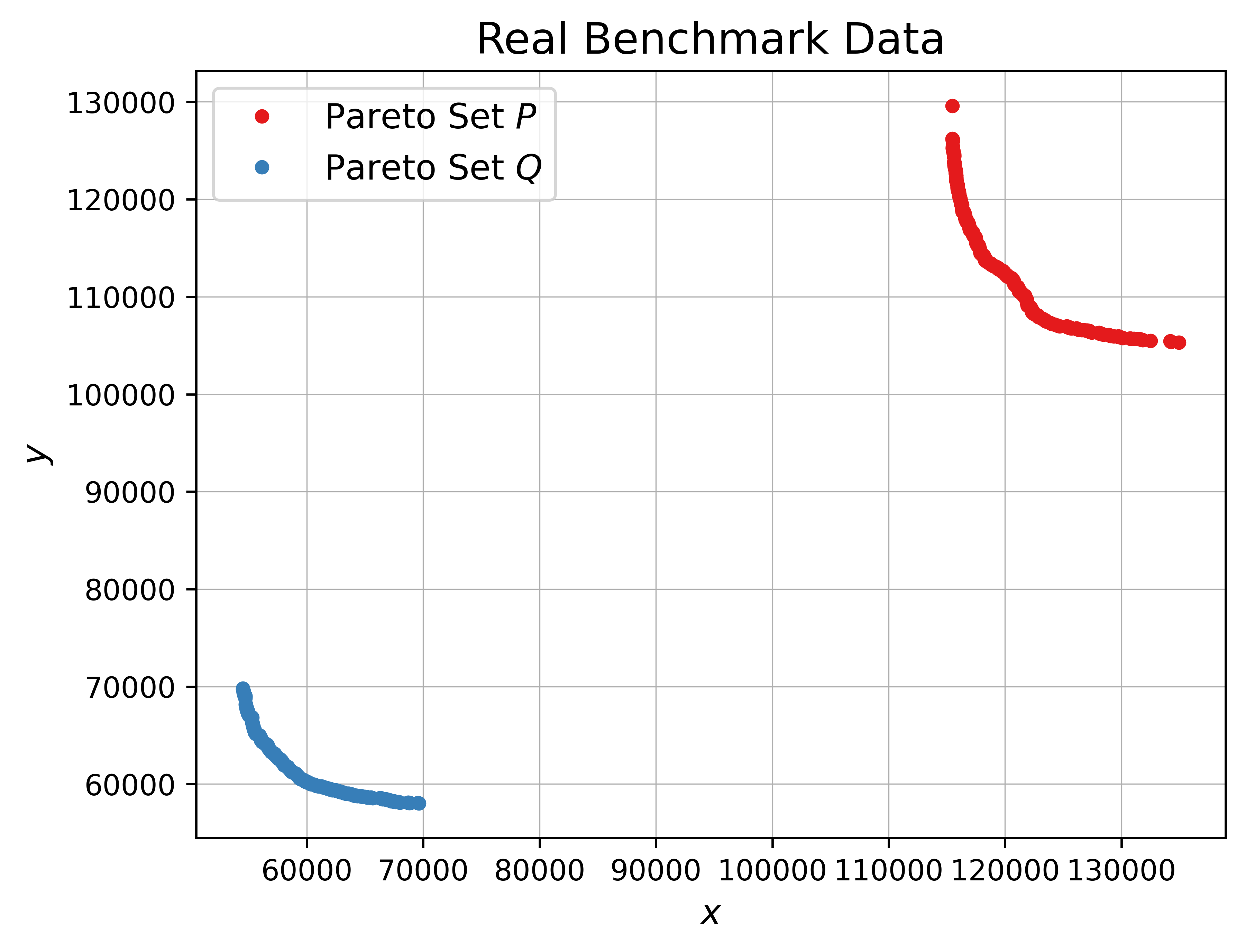
Recently, exact algorithms have been developed for Pareto sum computation with a running time in [13]. Naturally, the question arises whether this algorithm admits the best-possible time complexity for this problem or whether there is hope for designing asymptotically faster ones. The study of fine-grained complexity has emerged as a powerful framework for understanding the algorithmic complexity of problems within the class P. Using fine-grained reductions, the conjectured intractability of one key problem can be transferred to another problem, yielding a conditional lower bound on how fast the other problem can be solved. For the Pareto sum problem, it was recently shown that an algorithm with a running time in for , where denotes the output size, would disprove the 3-SUM hypothesis [15]. The conditional lower bound matches the complexity of known algorithms (up to subpolynomial factors), which renders the existence of subquadratic algorithms for Pareto sum (even with linear output sizes) unlikely.
However, in practical applications, Pareto sum instances of substantial input size and with output sizes frequently arise. On such instances, exact computation takes at least quadratic time, which is typically impractical. This motivates our study of approximation algorithms for Pareto sum. We define a point set to be an approximation of if for each element in there is a point in of “similar quality” (specifically, ) and each is indeed close to a point in (specifically for some ). This provides an additive approximation guarantee. This definition caters well to many practical applications of Pareto sum computation. For example, in bi-criteria route planning, the goal is to find the set of Pareto-optimal paths between the source and the target node with respect to two metrics. Route planning techniques for this setup heavily rely on Pareto sum computations and the number of resulting skyline points is oftentimes huge [13, 16, 25]. Thus, the goal is to reduce the number of Pareto-optimal paths to be considered within the algorithm and also as an output for the user. Multiplicative approximation algorithms tend to not work well in this scenario, because for paths with a value of zero or close to zero in one metric, even slightly suboptimal paths induce huge approximation factors. Additive approximations do not suffer from the same issue and are also much easier to interpret for a user (for example, if it is guaranteed that the reported route has at most 2 minutes of extra driving time). In this paper, we propose an efficient additive-approximation algorithm that allows one to trade running time against solution quality. We rigorously analyze its theoretical properties and also provide an extensive empirical study of its performance on synthetic and real data sets.
1.1 Related Work
The Pareto sum problem has already been extensively studied from a theoretical and practical perspective. A simple approach follows by computing the Minkowski sum explicitly and then applying general algorithms for skyline computation [17, 10]. In [18], the practical relevance of the problem was emphasized, and novel algorithms were proposed that achieve a subquadratic space consumption for certain input set structures. Algorithms with guaranteed output-sensitive space consumption were proposed in [13]. A simple Sort & Compare algorithm was proven to run in on input sets of size , and a sweep search algorithm to run in where denotes the output size. Experiments on synthetic instances and instances stemming from bi-criteria route planning in road networks confirm that these algorithms outperform those that fully compute the Minkowski sum and also the ones proposed in [18]. In [19], Pareto sum computation is used as a subroutine for multiobjective spanning tree or TSP computation which uses a tree decomposition as basis. For join nodes, an algorithm similar to Sort & Compare is used to obtain the desired combined result. In [14], several additional fine-grained complexity results for Pareto sum are provided. This includes a quadratic lower bound for Pareto sum computation even for under the 3-SUM hypothesis (which is even more believable than the previous min-plus convolution quadratic lower bound by [13], as the min-plus convolution hypothesis implies the -SUM hypothesis). Moreover, they established Pareto sum as a complete problem for a wide class of logical and geometric problems, further adding interest to the problem from the side of complexity theory.
1.2 Our Contributions
In this paper, we explore the degree to which the quadratic-time bottleneck for the Pareto sum problem – which is observable both in practice [13] and substantiated by conditional lower bounds [13, 14, 15] – can be circumvented by additively approximating Pareto sums. To this end, in Section 3, we formally introduce a natural relaxation of Pareto sums to -approximate Pareto sums: intuitively, is an approximation of the true Pareto set of if for any , we have an approximate point of “similar quality” (specifically, ). Conversely, any such is of similar quality to some actual point in (i.e., there are with ).222In fact, we often even achieve the stronger guarantee that , see Definition 5.
Crucially, our results rely on establishing a certain fine-grained equivalence between approximating Pareto sums and Bounded Monotone Min-Plus Convolution, the latter of which has received increasing interest in recent years [9, 11, 4, 6, 12]. This leads to the following theoretical results:
-
For any sets of at most points in , we can compute an -approximate Pareto sum in time . This leverages a remarkable algorithm due to Chi, Duan, Xie and Zhang [11] solving Bounded Monotone Min-Plus Convolution in strongly subquadratic time .
-
Conversely, we show that any -time algorithm for computing an -approximate Pareto sum would give a polynomial-factor improvement for Bounded Monotone Min-Plus Convolution. This establishes a fine-grained equivalence of the approximate Pareto sum and Bounded Min-Plus Convolution. Some approximation problems [8, 7] are known to be fine-grained equivalent to min-plus convolution, but this appears to be the first such connection for bounded monotone min-plus convolution.
-
We observe that slightly stronger approximation guarantees can be obtained if a witness-reporting version of Bounded Monotone Min-Plus Convolution can be achieved. Indeed, we show that such witnesses can be reported in strongly subquadratic time, by adapting a -time algorithm for Bounded Monotone Min-Plus Convolution [11] using techniques due to Alon and Naor [1].
Subsequently, we observe how beneficial our relaxation to approximate Pareto sums can be on realistic input sets. To this end, we empirically fine-tune and evaluate a number of different approaches, leading to the following results:
-
On synthetic and realistic inputs, we can approximate Pareto sums significantly more efficiently than computing them exactly. E.g., on generated data sets with points and coordinates in , computing an additive -approximation saves a computation time of up to three orders of magnitude. Furthermore, the size of the returned sets reduces significantly with coarser approximation parameters. Thus, we enable an effective choice of running time/solution size vs. approximation quality.
-
We focus on efficiently solving the Bounded Pareto sum problem, which denotes the special case in which all coordinates are integer values in – such instances occur naturally in our approximation algorithms (after a scaling step), but are of independent interest in bi-criteria optimizations with integral cost functions (e.g., in routing). Here, we empirically evaluate and compare several algorithmic approaches: (1) a natural adaptation of the Sort & Compare method of [13] to BucketSort & Compare, (2) a convex-pruning algorithm inspired by a fast algorithm for Near-convex Min-Plus Convolution [5], and (3) an algorithm based on a -time algorithm for Bounded Monotone Min-Plus Convolution [11] (which we will refer to as CDXZ algorithm). Perhaps surprisingly, we observe that depending on the class of inputs, either one of these approaches may outperform the others. This indicates that the (theoretical) connection between Pareto sums and Bounded Monotone Min-Plus convolution can also be exploited in practice to obtain practical algorithms (depending on the instances).
2 Bounded Pareto Sum
In this section, we prove our core reduction which is the basis for developing new algorithms for (approximate) Pareto sum computation. Throughout the paper, we abbreviate and use the interval notation for some , with . We say that a point dominates another point , if and with at least one coordinate being strictly smaller. A point set is called a Pareto set if it contains no dominated elements. For a point , we denote by and the and -coordinate of respectively. The Pareto front of a set , consists of the non-dominated points in . We are now ready to define the problems of interest.
Definition 1 (Bounded Pareto Sum).
Given Pareto sets of size with integer coordinates in , compute the set of non-dominated points in .
We remark that for bounded Pareto sum, we always have , as in a Pareto set the coordinates per dimension all need to be different.
Definition 2 (Bounded Monotone Min-Plus Convolution).
Given two monotone decreasing arrays and of size with positive entries bounded by . Compute an array , where for each , we have .
The following reduction is also illustrated in Figure 2 on a small Pareto sum instance333A similar construction has been noted by Chan and Lewenstein for the special case that and are connected sets i.e. all points in and have a neighboring point with distance 1; see [9, Remark 3.4].
Theorem 3.
An instance of bounded Pareto Sum with sets of size and entries can be reduced in time to an instance of bounded monotone min-plus convolution of two sequences of size with entries in .
Proof.
(Sketch.) We first shift all -coordinates in and so that the minimum -value becomes 0; this preserves all dominance relations in the Pareto sum.
Next, we construct two sequences and of length , initialized with value . For each point (resp. ), we set (resp. ) and then enforce monotonicity by a single left-to-right sweep: each entry is replaced by the minimum seen so far. After this step, (resp. ) equals the smallest -value among all points of (resp. ) with . This construction runs in time. Computing the min-plus convolution then yields, for each , exactly the smallest achievable -coordinate among all pairs , with . Thus contains all candidate points of the Pareto sum. A final linear-time sweep removes dominated entries from , leaving precisely the non-dominated pairs . Hence the Pareto sum of and can be obtained via a bounded monotone min-plus convolution instance computable in time. A more detailed proof can be found in the full version of the paper.
According to our theorem, if bounded monotone min-plus convolution can be solved in time for arrays of size with entries in , then we can solve bounded Pareto Sum in time . This makes algorithms for bounded monotone min-plus convolution applicable to Pareto Sum with little overhead to carry out the reduction and the back-transformation of the solution. By applying the algorithm of [11], we get:
Corollary 4.
Given two Pareto sets of size with integer entries , we can compute the Pareto sum of and in time
3 Additive Approximation of Pareto sum
In this section, we study additive approximation algorithms for Pareto sum with arbitrary real-valued inputs.
To formalize our notion of approximation, observe that the Pareto sum of and can be defined as the set satisfying the following three conditions: (1) dominates , i.e.., for every and , there exists some with , (2) and (3) is a Pareto set, i.e., pairwise non-dominating. To obtain an approximate Pareto set, it is only natural to relax the first condition by allowing an additive slack of in the domination inequality. Formally, we arrive a the following notion of approximation:
Definition 5 (-Approximative Pareto sum).
Let . We call a -approximation of the Pareto sum of if the following conditions hold:
-
1.
for all , there exists some with .
-
2.
,
-
3.
is a Pareto set.
Let us remark that we could have arrived at this definition via slightly adapting the notion of an approximative Pareto front by the authors in [20], which leans on the notion of Papadimitriou and Yannakakis [22]: Let denote the directed Hausdorff distance between and under some “distance” , i.e.,
Following [20], we call a set a -approximation for the Pareto set if . As a natural (asymmetric) “distance” measure that quantifies the disadvantage of taking over (w.r.t domination of other points), we define: Note that this measure is a more suitable definition than using, e.g., , which would unnaturally punish a point that is worse by in -direction, but much better (by ) in -direction. With this notion, is a -approximative Pareto sum of , if -approximates , (2) , and (3) is a Pareto set.
To obtain such an approximation, we proceed as follows: we first scale down the points of and by dividing the and -coordinates by a scaling parameter , creating the sets and . We additionally save a representative for each (rounded) point and in the original sets (we choose the one with minimal norm but any representative works). Then we compute the Pareto sum for the sets and and determine, from each , an approximate point using the representatives of and , which yields an approximate set . As we shall prove, this simple idea turns out to be conditionally optimal, by devising a fine-grained equivalence with bounded -convolution. This algorithm is formalized in Algorithm 1, which takes as input and a scaling factor , and returns a -approximation of the Pareto sum of and .
Lemma 6.
For any and , let denote and let denote the result of ApproximateParetoSum(). Then is a -approximation of the Pareto sum of .
Proof.
We first argue that the set computed in Algorithm 1 satisfies the relaxed domination condition with , specifically, that for all with , there exists some with . Indeed, for any , consider their rounded points , . By definition of the Pareto sum of , there must exist some with . We claim that approximately dominates , since
where we used for any rounded point in the first line, and for any and rounded point in the third line. We claim that the lemma follows: Filtering out dominated points in ensures that is a Pareto set (establishing Condition 3.), without affecting the domination condition (if dominates , then whenever , then , so is never needed to ensure the condition). Finally, clearly as any element of is explicitly given as for corresponding and .
Theorem 7.
Let denote the runtime of monotone min-plus convolution of arrays of size and entries bounded by with witness reporting. Given sets of points in , we can compute a -approximate Pareto sum in time .
Proof.
Given Lemma 6, it remains to show that ApproximateParetoSum( with can be computed in the desired running time. After -time preprocessing, the main step in Algorithm 1 is to compute the Pareto sum of . By our rounding, have integer coordinates in , and Theorem 3 is applicable to obtain and thus in time . Observe that is a set of size at most . Thus, we can compute its Pareto front in time , concluding the claim.
Corollary 8.
Given sets of points with real coordinates in and , we can compute an -approximation of the Pareto sum in time .
Proof.
Follows from the time algorithm of [11], and our witness reporting extension, described in the full version of the paper444We remark that it is very plausible that our witness reporting algorithm extends to the algorithm.. Let us also now show a lower bound, which will nicely complement Algorithm 1.
Theorem 9.
Let denote the running time of computing, given Pareto sets in with maximum coordinate bounded by , a -approximation of their Pareto sum, with witnesses. If there exists and such that whenever , then bounded monotone min-plus convolution can be computed in time , with witnesses.
Proof.
The proof is an adaptation of the reduction from min-plus convolution to Pareto sum given in [13]. Consider an arbitrary min-plus convolution instance with monotonicity (specifically, for all ) and entries in . We construct the sets of points
Consider a -approximation of the Pareto sum of with . By construction of the point sets, if a point -dominates a point , i.e., , then it already dominates , i.e., . Thus, is the true Pareto sum of , and we can extract the min-plus convolution of : By construction, for every , there must be a point in with -coordinate and -coordinate , revealing . The existence of a point with -coordinate for every follows by the decreasing values of . Also, witnesses for such points can be transferred.
Note that the constructed instance of Pareto sum Approximation consists of points in with coordinates bounded by and . Thus, if , then we can compute the min-plus convolution of in time , with witnesses.
Remark 10.
Even without witness reporting, we still get a fine-grained equivalence (for slightly weaker guarantees), by a minor adaptation of Algorithm 1 and Theorem 9. We relax the condition to the milder condition that each is in the vicinity of a point . More formally, for all there exist and such that Further details can be found in the full version of the paper.
4 Framework and Implementation
Our proposed additive approximation algorithm, presented in Algorithm 1, consists of scaling down the instance, computing the Pareto sum of the transformed point sets, and then scaling up the solution. The Pareto sum instance after scaling is captured by our definition of bounded Pareto sum. To compute its solution, we can obviously directly apply any Pareto sum algorithm. By virtue of Theorem 3, however, also any algorithm for bounded min-plus convolution translates to an algorithm for bounded Pareto sum when performing the required reduction and back-transformation of the solution. Thus, depending on whether we use an algorithm directly designed for Pareto sum or a convolution algorithm, the computation pipeline needs to be adapted. Figure 4 provides an overview of our framework.
In the following, we describe the algorithms of each category in more detail.
4.1 Algorithms for (bounded) Pareto sum
We start with the algorithms designed directly for Pareto sum computation.
Sort & Compare (SC) and Successive sweep search (SSS)
We implemented both state of the art algorithms for (general) Pareto sum computation from [13] as a baseline. In a nutshell, the Sort & Compare algorithm sorts the points in the sumset lexicographically and performs constant time dominance checks per point based on this ordering. Further details on the baselines can be found in the full version of the paper.
BucketSort & Compare (BSC)
For bounded integral Pareto sum, we can improve the Sort & Compare algorithm, by using bucketsort to sort the points, and then perform a direct update on the minimal -coordinate for each corresponding -coordinate. Further details can be found in the full version of the paper.
4.2 Algorithms for min-plus convolution
After the reduction to min-plus convolution, we can of course use the naive quadratic time algorithm for the latter. In the following, we discuss two more sophisticated and (potentially) faster convolution algorithms.
CDXZ Algorithm
We discuss a simplified version of the -algorithm [11, Section 4.1] for monotone bounded min-plus convolution in a detailed fashion in the full version of the paper. Using this algorithm in our Pareto sum reduction framework results in a running time of for bounded Pareto sum. Let us highlight the main improvements and simplifications we achieved.
-
We removed the segment tree data structure. Making use of a simpler enhanced min-plus convolution algorithm instead of using a segment tree with interval updates is simpler and improves the runtime theoretically and practically.
-
We improved the bound of , which was previously ranging from to The better bound of the constant , is insignificant in the theoretical analysis of the algorithm, but it plays an important role in the error correction part. Besides the initial polynomial multiplication of and , every other part of the algorithm in the error correction phase will be repeated -times, thus the better bound on will result on repeating these costly parts of the algorithm twice instead of thrice.
-
As the set can be of expected size (for the choice of , we do not save it explicitly like [11] suggests. In order to circumvent storing the set , we make an online computation of the polynomials simultaneously, updating the polynomials after having seen a new pseudo-witness on the fly.
We implemented the version without witness reporting, as the witness reporting algorithm would be too inefficient in practice. This leads to a weak approximation of the Pareto sum. For the multivariate polynomial multiplication, we perform a standard reduction to the univariate case, by turning and into univariate polynomials. Instead of FFT, we make use of the polynomial multiplication offered by the library FLINT [24], where the univariate polynomials are kept as lists. Instead of using binary search trees in the computation of , we performed a linear search, after saving for each possible modulo value the indices with . This turned out to be faster in the experiments. The parameters and are not fixed as the optimal theoretical runtime suggests. The choice of the parameters and are transferred to the choice of the scaling factor and the prime , which are now inputs of the implementation; see Figure 7 for the influence of these parameters on the runtime.
Convex Pruning (CP) algorithm
Bringmann and Cassis developed an algorithm for min-plus convolution, suited towards the case, where the arrays and are near-convex [5]. We implemented two versions of their algorithm with and without witness reporting. Our implementation is close to the descriptions in [5], with the main difference being that we did not use sparse convolutions, but rather an enhanced min-plus convolution computation, which works particularly well when the arrays and have few distinct entries. We precomputed groups of entries of the same value in and . More details on the enhanced min-plus convolution on the precise changes can be found in the full version of the paper.
4.3 Further engineering
Algorithm 1 has been implemented mostly matching its description, with small changes, which we describe now. When using a convolution algorithm within Algorithm 1, we also perform the needed reduction from bounded Pareto sum to monotone bounded min-plus convolution and the transformation backwards. The reduction closely follows the constructive proof of Theorem 3. At the end of Algorithm 1, instead of computing the Pareto front of the set by sorting, we do the following: For each newly inserted point, we look back and remove all points, which are dominated by this new point. This will work fast as the set is almost a Pareto set, so few corrections need to be made.
5 Experimental Evaluation
In the following, we evaluate our approximate algorithm with the different choices for bounded Pareto sum computation sketched above. While all algorithms are described for the case that and are of the same size , they also all work for differing sizes. Our code is written in C++. It was compiled with gcc using -O3. In our implementation of the CDXZ algorithm, we use routines from FLINT (Fast Library for Number Theory) [24]. All experiments were conducted on a single core of an AMD Threadripper 3970 with 256 GB of RAM. We set a time-out of one hour per run. Running times are always averaged over 10 runs.
Benchmarks.
We use three types of benchmarks in our evaluation. Two are synthetic to allow us to control instance properties, while the third benchmark consists of real data.
Benchmark 1: Instances with bounded range. First, we use an instance generator that allows us to fix and . Here, it is important to ensure to guarantee that there are enough distinct natural numbers in the range to construct a Pareto set. We use for . To efficiently create a strictly monotonically increasing sequence, we initialize an array with a counter for each . Then, we increment a randomly selected counter in each of rounds. Afterwards, we sweep over this array, starting at position 0, and perform the following operations: If , we set and . Here, entry 0 is assumed to be the successor of . We stop when all entries are 0 or 1 which happens after each entry has been considered at most twice. Then, for all , element is added to the sequence. This produces a valid sequence in time . Pareto sets can then be constructed by using two such sequences, one sorted increasingly for the -coordinates and the other one decreasingly for the corresponding -coordinates.
Benchmark 2: Function-based instance generator. For any strictly monotonically decreasing function defined on , sampling points provides us with a Pareto set. We use two base functions: the first uses and the second with a constant . We slightly perturb the points to have more input variability, while guaranteeing that pairwise non-dominance is upheld. We refer to the resulting instances as near-linear or near-curved.
See Figure 5 for an illustration. We note that by means of the perturbation, the resulting point sets are no longer convex.
Benchmark 3: Route planning instances. Finally, we also use real-world data sets for evaluation. The instances stem from bi-criteria route planning in line with [13]. Here, given a graph in which the edges are augmented with two cost values (in our case distance in meters and positive height difference in centimeters), the goal is to compute all Pareto-optimal paths from a source node to a target node . Using bi-directional search to answer such queries, or constructing a data structure which accelerates query answering [23], demands to combine and filter the set of Pareto-optimal paths from to some intermediate node , and from to the target . The cost pairs of these two path sets form our inputs and . The benchmark contains roughly 100000 instances based on randomly chosen and triples in a directed road network with one million nodes and two million edges. Note that the sizes of and might differ significantly in each instance.
Results for Exact Pareto Sum.
For a general comparison of the different algorithms for Bounded Pareto sum discussed in this paper, we first applied a scalability study on the range-bound instances with all point coordinates being integers, see Figure 6.
We observe huge performance differences. SSS is by far the slowest approach. Its theoretical performance is only subquadratic in case the output size is in . However, for the considered instances there are roughly output points. The BSC algorithm performs best and also significantly outperforms the plain SC algorithm. Even more remarkably, also the min-plus convolution based algorithms, naive and CP, outperform SC. While CDXZ beats SSS, it is a bit slower than SC on this instance type. As described in Section 4, our implementation of the CDXZ algorithm allows us to choose its parameters. We conducted a series of tests on synthetic instances of different sizes to determine a good parameter choice, see Figure 7 for an example.
We observe that the parameter values heavily impact the performance. Across all tested instances, scaling factors of and were among the top configurations. We therefore use those values in all subsequent experiments. We remark, though, that additional fine-tuning or choices adaptive to could potentially further improve the performance.
However, our main interest is in computing approximate solutions. In the following, we investigate how the algorithms perform when used as a plug-in in our approximation framework. In the remainder of the experiments, we focus on the BSC algorithm as well as the convolution based algorithms, as they outperform the baseline algorithms.
Results for Approximate Pareto Sum.
Next, we present comparative running time results of our approximation algorithm with different inner methods of Pareto sum computation applied to the scaled down inputs. For fair comparison, we use the non-witness reporting variants for all of them. Figures 8, 9, and 10 depict the results for range-bounded, near-linear and near-curve instances, respectively, using a value range of and a scaling factor of . Interestingly, for each input type, another algorithm performs best. For range-bounded instances, BSC is the fastest with CDXZ being second, while on near-linear instances CDXZ outperforms the other two methods. On near-curved instances, however, CP is clearly the best, beating the others by at least an order of magnitude.
The performance of CP relies on its ability to prune pairs, which on near-curved instances applies to up to 95% of total point pairs, see Figure 11.
Finally, we consider our third benchmark set, which consists of bi-criteria route planning instances of varying size. Figure 13 shows the running time and approximation quality of our algorithms for different scaling factors. We observe that BSC performs best with CP being a close second, especially for larger values of . They both improve on exact computation by over an order of magnitude and also stay well below the theoretical additive approximation bound of .
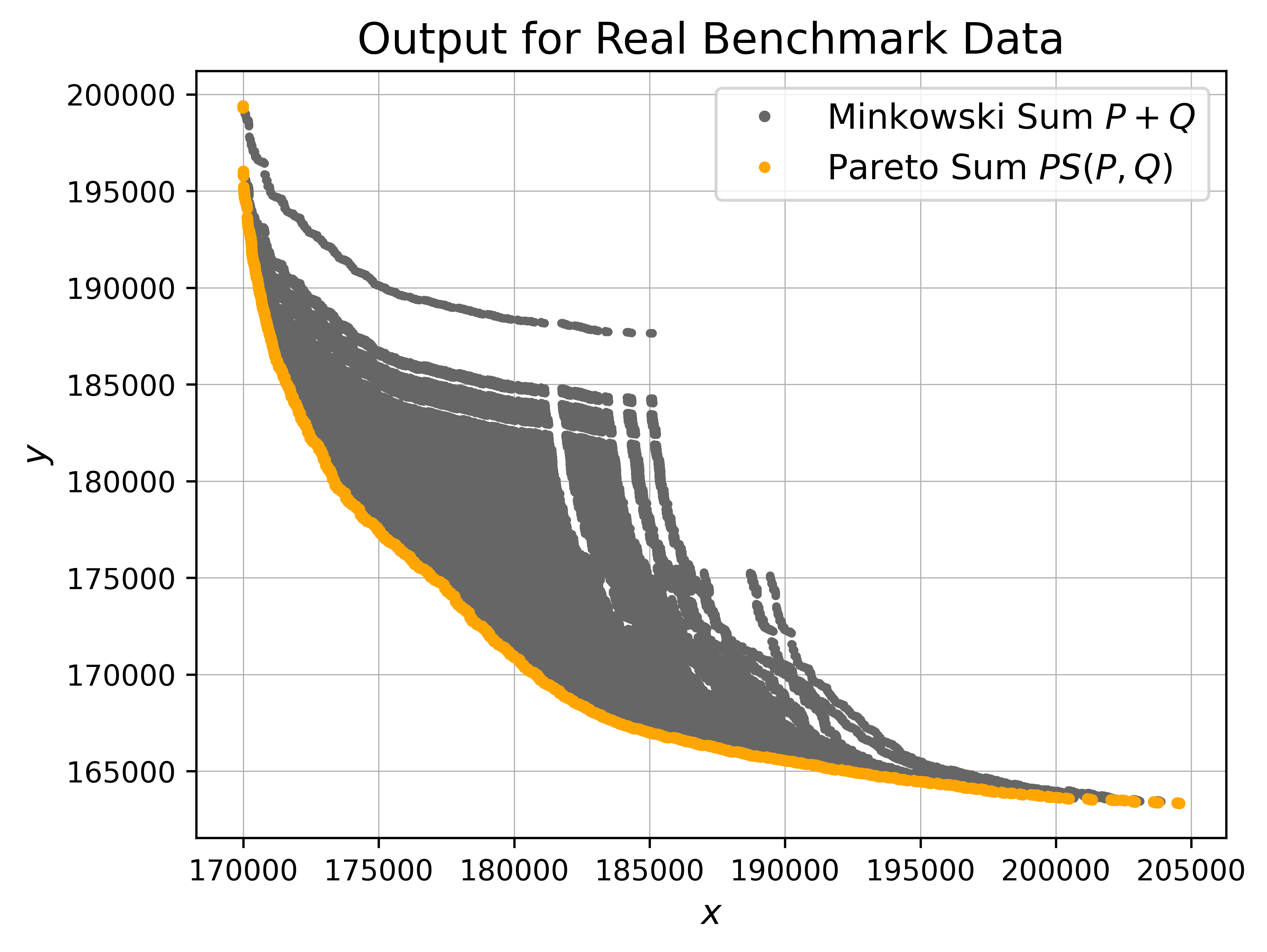
Examples of approximate solutions can be found in Figures 14.
One can see that even when choosing a larger , the Pareto sum is still well represented by the computed solution. Indeed, larger values of are quite reasonable in our application. For example, a route that is up to 100 meters longer than another one is almost indistinguishable to a user if the total route length is anyway in the orders of kilometers.
Furthermore, the user usually does not want to be presented with hundreds of routing options, but a concise and diverse set of reasonable options. This is achievable with our approach, as we can not only reduce the running time with larger but also the output size, see Figures 15 and 12. Clearly, our algorithm provides good trade-offs between running time and solution quality, which allows one to choose the best depending on the application.
6 Future Work & Discussion
We have established that fine-grained reductions are not only a means to obtain theoretical intractability results, but also a tool to efficiently solve problems via reductions to other problems for which fast algorithms are implemented and engineered. To further foster (bounded monotone) min-plus convolution as a core primitive, it would be interesting to know whether the algorithm [11, Section 4.2], admits an efficient implementation. The main drawback right now is that it needs calls to the monotone bounded min-plus function, and that the constant is much larger than in the algorithm we implemented. We believe that the CP algorithm can benefit from practical sparse convolution algorithms, especially on near-linear inputs. Is it possible to engineer fast sparse convolution algorithms in practice? Finally, can we leverage our min-plus convolution results to obtain practical improvements for knapsack [4, 6] or the tree sparsity problem [21, 2]?
References
- [1] Noga Alon and Moni Naor. Derandomization, witnesses for boolean matrix multiplication and construction of perfect hash functions. Algorithmica, 16(4/5):434–449, 1996. doi:10.1007/BF01940874.
- [2] Arturs Backurs, Piotr Indyk, and Ludwig Schmidt. Better approximations for tree sparsity in nearly-linear time. In Philip N. Klein, editor, Proceedings of the Twenty-Eighth Annual ACM-SIAM Symposium on Discrete Algorithms, SODA 2017, Barcelona, Spain, Hotel Porta Fira, January 16-19, pages 2215–2229. SIAM, 2017. doi:10.1137/1.9781611974782.145.
- [3] Karl Bringmann. Approximating subset sum ratio faster than subset sum. In David P. Woodruff, editor, Proceedings of the 2024 ACM-SIAM Symposium on Discrete Algorithms, SODA 2024, Alexandria, VA, USA, January 7-10, 2024, pages 1260–1277. SIAM, 2024. doi:10.1137/1.9781611977912.50.
- [4] Karl Bringmann and Alejandro Cassis. Faster knapsack algorithms via bounded monotone min-plus-convolution. In Mikolaj Bojanczyk, Emanuela Merelli, and David P. Woodruff, editors, 49th International Colloquium on Automata, Languages, and Programming, ICALP 2022, July 4-8, 2022, Paris, France, volume 229 of LIPIcs, pages 31:1–31:21. Schloss Dagstuhl – Leibniz-Zentrum für Informatik, 2022. doi:10.4230/LIPIcs.ICALP.2022.31.
- [5] Karl Bringmann and Alejandro Cassis. Faster 0-1-knapsack via near-convex min-plus-convolution. In Inge Li Gørtz, Martin Farach-Colton, Simon J. Puglisi, and Grzegorz Herman, editors, 31st Annual European Symposium on Algorithms, ESA 2023, Amsterdam, The Netherlands, September 4-6, 2023, volume 274 of LIPIcs, pages 24:1–24:16. Schloss Dagstuhl – Leibniz-Zentrum für Informatik, 2023. doi:10.4230/LIPIcs.ESA.2023.24.
- [6] Karl Bringmann, Anita Dürr, and Adam Polak. Even faster knapsack via rectangular monotone min-plus convolution and balancing. In Timothy M. Chan, Johannes Fischer, John Iacono, and Grzegorz Herman, editors, 32nd Annual European Symposium on Algorithms, ESA 2024, September 2-4, 2024, Royal Holloway, London, United Kingdom, volume 308 of LIPIcs, pages 33:1–33:15. Schloss Dagstuhl – Leibniz-Zentrum für Informatik, 2024. doi:10.4230/LIPIcs.ESA.2024.33.
- [7] Karl Bringmann, Ahmed Ghazy, and Marvin Künnemann. Exploring the Approximability Landscape of 3SUM. In Timothy Chan, Johannes Fischer, John Iacono, and Grzegorz Herman, editors, 32nd Annual European Symposium on Algorithms (ESA 2024), volume 308 of Leibniz International Proceedings in Informatics (LIPIcs), pages 34:1–34:15, Dagstuhl, Germany, 2024. Schloss Dagstuhl – Leibniz-Zentrum für Informatik. doi:10.4230/LIPIcs.ESA.2024.34.
- [8] Karl Bringmann and Vasileios Nakos. A fine-grained perspective on approximating subset sum and partition. In Dániel Marx, editor, Proceedings of the 2021 ACM-SIAM Symposium on Discrete Algorithms, SODA 2021, Virtual Conference, January 10 - 13, 2021, pages 1797–1815. SIAM, 2021. doi:10.1137/1.9781611976465.108.
- [9] Timothy M. Chan and Moshe Lewenstein. Clustered integer 3sum via additive combinatorics. In Rocco A. Servedio and Ronitt Rubinfeld, editors, Proceedings of the Forty-Seventh Annual ACM on Symposium on Theory of Computing, STOC 2015, Portland, OR, USA, June 14-17, 2015, pages 31–40. ACM, 2015. doi:10.1145/2746539.2746568.
- [10] Wei-Mei Chen, Hsien-Kuei Hwang, and Tsung-Hsi Tsai. Maxima-finding algorithms for multidimensional samples: A two-phase approach. Computational Geometry, 45(1-2):33–53, 2012. doi:10.1016/J.COMGEO.2011.08.001.
- [11] Shucheng Chi, Ran Duan, Tianle Xie, and Tianyi Zhang. Faster min-plus product for monotone instances. In Stefano Leonardi and Anupam Gupta, editors, STOC ’22: 54th Annual ACM SIGACT Symposium on Theory of Computing, Rome, Italy, June 20 - 24, 2022, pages 1529–1542. ACM, 2022. doi:10.1145/3519935.3520057.
- [12] Weiming Feng and Ce Jin. Approximately counting knapsack solutions in subquadratic time. In Yossi Azar and Debmalya Panigrahi, editors, Proceedings of the 2025 Annual ACM-SIAM Symposium on Discrete Algorithms, SODA 2025, New Orleans, LA, USA, January 12-15, 2025, pages 1094–1135. SIAM, 2025. doi:10.1137/1.9781611978322.32.
- [13] Daniel Funke, Demian Hespe, Peter Sanders, Sabine Storandt, and Carina Truschel. Pareto sums of pareto sets: Lower bounds and algorithms. Algorithmica, pages 1–34, 2025.
- [14] Geri Gokaj and Marvin Künnemann. Completeness theorems for k-sum and geometric friends: Deciding fragments of linear integer arithmetic. In Raghu Meka, editor, 16th Innovations in Theoretical Computer Science Conference, ITCS 2025, January 7-10, 2025, Columbia University, New York, NY, USA, volume 325 of LIPIcs, pages 55:1–55:25. Schloss Dagstuhl – Leibniz-Zentrum für Informatik, 2025. doi:10.4230/LIPIcs.ITCS.2025.55.
- [15] Geri Gokaj, Marvin Künnemann, Sabine Storandt, and Carina Truschel. (multivariate) k-sum as barrier to succinct computation. In Anne Benoit, Haim Kaplan, Sebastian Wild, and Grzegorz Herman, editors, 33rd Annual European Symposium on Algorithms, ESA 2025, September 15-17, 2025, Warsaw, Poland, volume 351 of LIPIcs, pages 42:1–42:19. Schloss Dagstuhl – Leibniz-Zentrum für Informatik, 2025. doi:10.4230/LIPIcs.ESA.2025.42.
- [16] Boris Goldin and Oren Salzman. Approximate bi-criteria search by efficient representation of subsets of the pareto-optimal frontier. In Proceedings of the International Conference on Automated Planning and Scheduling, volume 31, pages 149–158, 2021. URL: https://ojs.aaai.org/index.php/ICAPS/article/view/15957.
- [17] David G Kirkpatrick and Raimund Seidel. Output-size sensitive algorithms for finding maximal vectors. In Proceedings of the First Annual Symposium on Computational Geometry, pages 89–96, 1985. doi:10.1145/323233.323246.
- [18] Kathrin Klamroth, Bruno Lang, and Michael Stiglmayr. Efficient dominance filtering for unions and minkowski sums of non-dominated sets. Computers & Operations Research, 163:106506, 2024. doi:10.1016/J.COR.2023.106506.
- [19] Joshua Marc Könen, Heiko Röglin, and Tarek Stuck. Parameterized Algorithms for Computing Pareto Sets. In Anne Benoit, Haim Kaplan, Sebastian Wild, and Grzegorz Herman, editors, 33rd Annual European Symposium on Algorithms (ESA 2025), volume 351 of Leibniz International Proceedings in Informatics (LIPIcs), pages 105:1–105:15, Dagstuhl, Germany, 2025. Schloss Dagstuhl – Leibniz-Zentrum für Informatik. doi:10.4230/LIPIcs.ESA.2025.105.
- [20] Julien Legriel, Colas Le Guernic, Scott Cotton, and Oded Maler. Approximating the pareto front of multi-criteria optimization problems. In Javier Esparza and Rupak Majumdar, editors, Tools and Algorithms for the Construction and Analysis of Systems, 16th International Conference, TACAS 2010, Held as Part of the Joint European Conferences on Theory and Practice of Software, ETAPS 2010, Paphos, Cyprus, March 20-28, 2010. Proceedings, volume 6015 of Lecture Notes in Computer Science, pages 69–83. Springer, 2010. doi:10.1007/978-3-642-12002-2_6.
- [21] Marcin Mucha, Karol Wegrzycki, and Michal Wlodarczyk. A subquadratic approximation scheme for partition. In Timothy M. Chan, editor, Proceedings of the Thirtieth Annual ACM-SIAM Symposium on Discrete Algorithms, SODA 2019, San Diego, California, USA, January 6-9, 2019, pages 70–88. SIAM, 2019. doi:10.1137/1.9781611975482.5.
- [22] Christos H. Papadimitriou and Mihalis Yannakakis. On the approximability of trade-offs and optimal access of web sources. In 41st Annual Symposium on Foundations of Computer Science, FOCS 2000, Redondo Beach, California, USA, November 12-14, 2000, pages 86–92. IEEE Computer Society, 2000. doi:10.1109/SFCS.2000.892068.
- [23] Sabine Storandt. Route planning for bicycles—exact constrained shortest paths made practical via contraction hierarchy. In Proceedings of the International Conference on Automated Planning and Scheduling, volume 22, pages 234–242, 2012.
- [24] The FLINT team. FLINT: Fast Library for Number Theory, 2025. Version 3.3.1, https://flintlib.org.
- [25] Carina Truschel and Sabine Storandt. Multi-Criteria Route Planning with Little Regret. In Jonas Sauer and Marie Schmidt, editors, 25th Symposium on Algorithmic Approaches for Transportation Modelling, Optimization, and Systems (ATMOS 2025), volume 137 of Open Access Series in Informatics (OASIcs), pages 13:1–13:20, Dagstuhl, Germany, 2025. Schloss Dagstuhl – Leibniz-Zentrum für Informatik. doi:10.4230/OASIcs.ATMOS.2025.13.