Estimating the Persistent Homology of -Valued Functions Using Function-Geometric Multifiltrations

Abstract
Given an unknown -valued function on a metric space , can we approximate the persistent homology of from a finite sampling of with known pairwise distances and function values? This question has been answered in the case , assuming is Lipschitz continuous and is a sufficiently regular geodesic metric space, and using filtered geometric complexes with fixed scale parameter for the approximation. In this paper we answer the question for arbitrary , under similar assumptions and using function-geometric multifiltrations. Our analysis offers a different view on these multifiltrations by focusing on their approximation properties rather than on their stability properties. We also leverage the multiparameter setting to provide insight into the influence of the scale parameter, whose choice is central to this type of approach. From a practical standpoint, we show that our approximation results are robust to input noise, and that function-geometric multifiltrations have good statistical convergence properties. We also provide an algorithm to compute our estimators, and we use its implementation to conduct extensive experiments, on both synthetic and real biological data, in order to validate our theoretical results.
Keywords and phrases:
Topological data analysis, multi-parameter persistent homology, function-Rips multifiltrationFunding:
David Loiseaux: Inria Action Exploratoire PreMediT (Precision Medicine using Topology).Copyright and License:
![[Uncaptioned image]](x1.png) © Ethan André, Jingyi Li, David Loiseaux, and Steve Oudot; licensed under Creative Commons License CC-BY 4.0
© Ethan André, Jingyi Li, David Loiseaux, and Steve Oudot; licensed under Creative Commons License CC-BY 4.0
2012 ACM Subject Classification:
Mathematics of computing Algebraic topologyEditors:
Hee-Kap Ahn, Michael Hoffmann, and Amir NayyeriSeries and Publisher:
 Leibniz International Proceedings in Informatics, Schloss Dagstuhl – Leibniz-Zentrum für Informatik
1 Introduction
Let be a metric space and a function, both unknown. Suppose we are given a finite point cloud sampled from , such that the pairwise distances between the points of are known, as well as the function values at the points of . Given this input, can we approximate the persistent homology of (i.e., the persistence module induced in homology from the multifiltration of by the sublevel sets of ) with provable guarantees? This question was addressed in [10] in the case . The authors proposed an estimator based on a nested pair of Rips complexes , where is a user-defined parameter, which they filtered by the values of at the vertices using lower-star filtrations. The estimator was then the image of the morphism of -parameter persistence modules induced in homology by the inclusion . We denote by this estimator. Assuming both the domain and the function are sufficiently regular (typically, is a compact geodesic metric space with positive convexity radius , and is -Lipschitz continuous), and is an -sample of in the geodesic distance for some small enough value of (specifically, ), they proved that the estimator is -interleaved with for any choice of parameter within the range . Thus, in cases where is known or can be estimated reliably, one can get an -interleaving with the target , hence an -matching with its barcode, by the algebraic stability theorem [2, 8, 9]. Under a reasonable sampling model, goes to zero as the number of sample points goes to infinity, hence so does the approximation error, which means that the proposed estimator is consistent. This approach has since been applied in various contexts, notably in clustering where the algorithm ToMATo [11] is an instance of the method in homology degree . However, two fundamental questions were left open in [10, 11]:
-
Q1
how to estimate , or to choose parameter directly, when is unknown;
-
Q2
how to generalize the approach to arbitrary , i.e., to vector-valued functions .
Q2 is precisely the question we asked at the beginning. Q1 is related to the general problem of scale parameter estimation, which has received a lot of attention in statistics, including in the context of topological data analysis (TDA) – see e.g. [4, 6, 23].
Contributions
In this paper we address both Q1 and Q2 using a unified persistence-based approach.
For Q2 we study the extension of the estimator from [10] to vector-valued functions , where the codomain is equipped with the product order, and we generalize its approximation guarantee to this setting. For the sake of generality we assume to be -continuous for some modulus of continuity , that is: for any , where is a non-decreasing subadditive function such that goes to as does. This includes Lipschitz or Hölder continuous functions as special cases. Under this assumption, our first main result (Theorem 3) states that the estimator is -interleaved with its target for any choice of within the range , under the same regularity condition on and -sampling condition on as before. Our proof takes inspiration from the one in [10] but uses a new, purely diagrammatic formulation that clarifies it and makes it hold for any .
For Q1 we propose two complementary approaches. The first one infers a relevant choice of under an appropriate statistical model. This model assumes the points are sampled i.i.d. according to some unkown probability distribution that is supposed to be -standard. When parameters are known, we show that there is an explicit optimal choice for parameter , as a function of the sample size , that makes the sequence of approximations a quasi-minimax estimator of . When are unknown, as would generally be the case in practice, we show that can be effectively estimated by some under our statistical model, so that the sequence is again a quasi-minimax estimator of . These statements are summarized in Theorem 5.
Our second approach to addressing Q1 is meant for cases where our statistical model does not hold and cannot be estimated reliably. We follow the general philosophy underpinning persistent homology by letting vary over and treating it as an extra parameter for persistence. This means that our estimator now becomes the -parameter persistence module indexed over , where the notation indicates that the Rips parameter is also a filtration parameter. In order to enable comparisons, the target must also be extended to , which we do by taking its left Kan extension along the poset embedding . The extension merely contains copies of in each vertical hyperplane , connected by horizontal identities, as illustrated in Figure 1. Our third main result (Theorem 6) states that the -dimensional interleavings happening between and inside each vertical hyperplane for commute with the horizontal morphisms in and in , so that, within any vertical slab with , they all together form a vertical -interleaving (i.e., an -interleaving along the direction in ) between and .
Since vertical interleavings are stronger than ordinary interleavings (Remark 1), Theorem 6 not only provides approximation guarantees for any interleaving-stable invariant of by the corresponding invariant of , but it also offers refined statements for invariants that behave in a particular way under vertical interleavings, such as for instance multigraded Betti numbers as proven in the full version [1] and illustrated in Figure 2.
In practice, function values may be corrupted with measurement noise, meanwhile geodesic distances may have to be approximated from the input data. Our framework can account for these imprecisions by suitably adapting the parameters of the estimators and their approximation bounds (see the full version [1, Section 3.3]).
Still for practical purposes, we discuss the computation of our estimators, in particular we provide an algorithm for computing a free presentation of , and thus also of for any fixed , in time that is comparable to that of computing a free presentation of the persistent homology of a single multifiltration. From a free presentation, a variety of invariants, including multigraded Betti numbers, can be derived using existing software. We have implemented our algorithm and used it in our experiments.
Structure of the paper
We provide background material in Section 2. Our problem statement, estimators, and main results are detailed in Section 3. In Section 4 we discuss algorithmic aspects. Finally, in Section 5 we present experimental results that illustrate our theoretical guarantees and we investigate additional properties of our estimators. Further algorithmic details, as well as the proofs of our main results, can be found in the full version [1].
2 Background
We assume some familiarity with basic category theory, algebraic topology, measure theory, and topological data analysis. Let denote the category of topological spaces, and (resp. ) the category of finite-dimensional (resp. all) vector spaces over a fixed field . We also fix an arbitrary degree in homology, denoted by , and we write for singular homology groups in degree with coefficients in .
Filtrations and persistence modules
We see as the product of copies of the real line, equipped with the product order noted . Thus, two points satisfy whenever for all . We denote by the downset , and by the upset . An -parameter filtration is a functor whose constituent maps are inclusions, which means that we have a topological space for all and an inclusion for all . An -parameter persistence module is a functor , which means that we have a -vector space for all and a -linear map for all , such that and for all . A morphism of persistence modules is a natural transformation between functors, i.e., a family of linear maps such that for all .
Geodesic metric spaces
Throughout the paper, unless otherwise specified, is a compact geodesic metric space. This means that, for all , there is a shortest continuous path from to in , of length equal to . In particular, the space is path-connected. Let be a finite set of points of . Given , we say is a geodesic -sample of if , where denotes the Hausdorff distance in . Define as the open geodesic ball centered at with radius , given by A ball is said to be convex if, for any pair of points and in , the shortest path in that connects to is unique and included in . Let , and let . This quantity, called the convexity radius of , plays an important role because intersections of convex sets are convex and therefore contractible, so the Nerve Lemma [13, Corollary 4G.3] applies to unions of balls of radii less than .
Functional and geometric filtrations
Given a geodesic metric space and a function , the sublevel filtration of is defined by for all . The persistent homology of (and, by extension, of ) is the persistence module (also written ) defined by and for all .
Given a finite set of points in X, and a real parameter , we call -offset of the union of open geodesic balls . We call -Čech Complex of the nerve of the collection of balls , defined as the abstract simplicial complex . For , the balls and their intersections are either empty or convex, so the Nerve Lemma [13, Corollary 4G.3] ensures that the homology groups and are isomorphic. We call -Rips complex of the abstract simplicial complex . Čech and Rips complexes of are related as follows:
Interleavings
Let be a fixed vector, and let . Given any functors to some category , we say and are -interleaved if there are two natural transformations and such that and . Here, denotes the -shift functor, defined on objects by and on morphisms by for all . Meanwhile, and denote the natural morphisms from and to their respective -shifts, defined by and for all . The -interleaving distance is defined as follows:
In the following, we consider two specific types of interleavings:
-
1.
Ordinary interleavings: Let . Then, -interleavings are ordinary -interleavings from the TDA literature, and is called the ordinary interleaving distance.
-
2.
Vertical interleavings: Let Then, -interleavings are called vertical -interleavings, and is called the vertical interleaving distance.
Remark 1.
Vertical interleaving implies ordinary interleaving. Indeed, the vertical interleaving maps can be composed with the horizontal structure morphisms of the modules to form an ordinary interleaving. The amplitude of the interleaving does not change in the process. Therefore, vertical interleaving is a stronger condition than ordinary interleaving.
3 Problem statement and main results
Let be a compact geodesic metric space with positive convexity radius , and let be a continuous function. Here, is equipped with the -norm. Both and are unknown. By the Heine–Cantor Theorem, admits a modulus of continuity . Neither nor need to be known, as they only play a role in our bounds and not in our constructions. The function is not assumed to be pointwise finite-dimensional (i.e., finite for every ), however our assumptions imply a form of tameness for the persistence module (see Corollary 4).
Our input is a finite point cloud such that , the restriction of to , is known, as well as the pairwise geodesic distances between the points . The problem we address is that of estimating , the persistent homology of the sublevel filtration of , from our input. For this we assume that is a geodesic -sample of , for some possibly unknown that we assume to be small enough compared to the convexity radius .
To build our estimator, we first construct the function-Rips multifiltration from the restriction of to . Then, following [10], our estimator is a smoothed version of , denoted by and defined formally as the image of the morphism of persistence modules induced in homology by the inclusion of the filtration into its horizontal rescaling by a factor of , that is:
where
Remark 2.
It is known that a single Rips complex of a finite sampling can recover the homological type of a sufficiently regular underlying continuous space [14, 16]. Yet, in full generality it takes a pair of Rips complexes with parameters within a factor of at least of each other to do so [7]. Similarly, it was recently shown that itself can approximate provided has curvature bounded above locally [22]. Yet, it is unknown whether the same holds in our more general setting, which is why we use .
In the course of our analysis of the behavior of , we will consider intermediate constructions, namely the persistent homologies of:
-
the function-offset filtration ;
-
the function-Čech filtration .
These can also serve as alternative estimators when they can be built, for instance – in the case of – when we can test whether finitely many open geodesic balls intersect.
We use our estimators in two types of scenarios: (1) when we have an estimate of the value for which is an -sample of , and (2) when we do not have such an estimate.
3.1 Estimating with known
Suppose we know or some reasonable estimate. Then we can approximate our target by restricting our estimators to a vertical hyperplane for a suitable choice of parameter . We denote these restrictions respectively by , and .
Theorem 3.
Let be a compact geodesic space, let be an -continuous function for some modulus of continuity , and let be a finite geodesic -sample of . Then:
-
(i)
for , the modules and are ordinarily -interleaved;
-
(ii)
for , the modules and are ordinarily -interleaved;
-
(iii)
for , modules and are ordinarily -interleaved.
The proof of this result is given in the full version [1, Section 4]. The conclusion still holds under noisy input function values or geodesic distances, as detailed in [1, Section 3.3].
Theorem 3 can be read in two different ways. First, when the modulus of continuity is known, we obtain explicit bounds on the interleaving distance between our estimators and the target . Second, when we only know that is continuous, the Heine–Cantor Theorem implies that admits some modulus of continuity , and even without knowning that , we are guaranteed by Theorem 3 that our estimators converge to as goes to zero under suitable choices of parameter .
When is known exactly, the best choice for is the lower bound of its admissible interval, i.e., in Items i and ii and in Item iii. When is only known approximately, the admissible interval provides some leeway for the choice of .
An immediate consequence of Theorem 3 is that -stable invariants computed on our estimators approximate the corresponding invariants defined on the target . For instance, the approximation guarantee obtained for the multigraded Betti numbers of is given in the full version [1, Corollary 3.3].
Another consequence of Theorem 3 (i) is that, under our assumptions, the persistence module satisfies the following form of tameness, as proven in the full version [1].
Corollary 4.
Let be as in Theorem 3. Then the module is tame in the sense that the rank is finite for all with for each .
Suppose now the points of are i.i.d. samples drawn from some unknown probability measure supported on . In this setting, standard statistical techniques can be used to estimate with high probability, then Theorem 3 can be applied to get statistical estimates of or of any -stable invariant thereof. We summarize our results in Theorem 5. The relevant statistical background and definitions are provided in the full version [1, Section 2], together with the analysis of the statistical estimators [1, Section 6].
Theorem 5.
Let , and be as in Theorem 3. Assume that the convexity radius satisfies , that the modulus of continuity has a controlled vanishing rate as , and that the points of are i.i.d. samples drawn from some unknown -standard probability measure whose support is the entire space .
-
(i)
Suppose are known. Let . Then, the sequences of approximations , and of are -quasi-minimax consistent estimators of in the following sense: their expected interleaving distances to are at most a constant times ; meanwhile, in the worst case over as above, for any other estimator of , the supremum over all -standard measures of the expected interleaving distance between the estimator and its target is at least a constant times .
-
(ii)
Suppose are unknown, and assume further that is a compact smooth manifold and that the measure decomposes as , where and is absolutely continuous with respect to the uniform measure on , with a positive density on . Then, there is an explicit sequence of random positive numbers such that the induced plug-in estimators , , and are -quasi-minimax consistent estimators of .
3.2 Estimating with unknown
When is unknown and cannot be effectively estimated – for instance when the assumptions in Theorem 5 are not satisfied, we adopt the traditional approach in persistence theory which is to not fix the scale parameter but rather to consider it as an extra filtration parameter. This means using the full -parameter modules , and as estimators. In order to state approximation results, we extend our target to a persistence module over by taking its left Kan extension along the poset embedding given by for all . Since the category is small and the category is cocomplete, is well-defined as a functor , and given pointwise by the colimit formula [19]:
| (1) |
Moreover, has structural morphisms that are identity maps horizontally (i.e., along the first coordinate axis) and the structural morphisms of vertically (i.e., along any direction orthogonal to the first coordinate axis), as illustrated in Figure 1.
Theorem 6.
Let , , , and as in Theorem 3. Then:
-
(i)
for , within the slab , the restricted modules and are vertically -interleaved;
-
(ii)
for , within the slab , the restricted modules and are vertically -interleaved;
-
(iii)
for , within the slab , the restricted modules
and are vertically -interleaved.
The proof is given in the full version [1, Section 5]. Similar to Theorem 3, the conclusion still holds under noisy input function values or geodesic distances – see [1, Section 3.3].
This approximation result encapsulates the previous one in the sense that restricting the estimators to the vertical hyperplane for recovers Theorem 3. However, the result says something deeper, namely: that the interleavings in the vertical hyperplanes , for ranging over (resp. ), commute with the horizontal structural morphisms of the modules, so that they all together form a vertical interleaving in the slab (resp. ). Intuitively, this means that prominent features in are not just present in at individual scales in the range , but that they persist across large ranges of scales in . In particular, they are not ephemeral in and can be captured by stable invariants.
In terms of approximation accuracy, the result says that, the more one looks to the left (i.e., toward small positive values of ) in the parameter space , the more precisely the estimators approximate the target, until some point where becomes too small and the approximation breaks down. On the opposite side, the more one looks to the right (i.e., toward large values of ), the more the estimators drift away from the target, until again the approximation eventually breaks down if the estimator is or . See Figure 2 for an illustration, and Figure 3 for a comparison of Theorem 6 with Theorem 3.

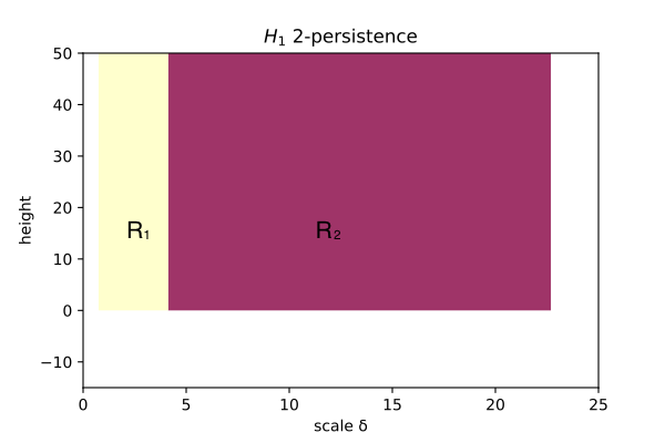

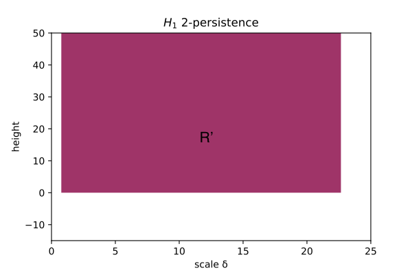
Theorem 6, like its counterpart Theorem 3, implies that provably -stable invariants computed from our estimators approximate the corresponding invariants defined on their target, which this time is . And since the interleaving is now vertical – hence stronger than an ordinary interleaving according to Remark 1, we can get more precise statements for some invariants. For instance, the induced bottleneck matching on multigraded Betti numbers is vertical, as proven in the full version [1] and illustrated in Figure 2.
4 Estimators Computation
Our main estimators, and , derive from the function Rips filtration , whose computation is standard – see [1, Section 7] for details. Here we focus on the computation of invariants once has been built. The difficulty is that our estimators do not come from a single filtration, but from the inclusion of two nested filtrations sitting inside . For some invariants, such as the Hilbert function or rank invariant, existing algorithms adapt straightforwardly [5]. However, for minimal free presentations – from which many invariants, including multigraded Betti numbers, derive – there is no efficient existing algorithm, except in special situations such as when homology in degree is considered, see the full version [1, Section 7.2.3] for details.
To address this, we provide an algorithm for the general problem of computing a free presentation of the image of any morphism of finitely presented persistence modules , and then we apply it to the special case of . Here we merely outline the mathematical construction of a free presentation of , which explains our approach. The algorithmic details and pseudocode are provided in [1, Section 7]. Note that a simpler variant to obtain a free presentation of the cokernel of appeared in [12, Proposition 4.14].
Let be a morphism between finitely presented persistence modules, with respective free presentations and . Since is projective, we can lift to a map so that the following diagram commutes:
| (2) |
From this diagram, we can derive a free presentation of as follows. Consider the pullback of the subdiagram , i.e., the kernel of the morphism , where for any . Let and denote the canonical projections from to and , respectively. Next, let be the free cover of , yielding the surjection . We illustrate these morphisms in the following commutative diagram, where form a pullback square:
| (3) |
This diagram yields a free presentation of as follows (proof is in the full version [1]):
Proposition 7.
The sequence is exact, where comes from the factorization of through its image . Consequently, the morphism is a free presentation of , and in fact a finite free presentation.
5 Experiments
In this section, we illustrate our approximation and convergence results through practical experiments on both synthetic and real-world datasets.
5.1 Toy examples
We validate the claims in Theorems 3 and 6 through a simple example consisting of two circles with distinct radii and concentration levels, as shown in Figure 4 (a). In Figure 4 (b) we analyze the error between the estimator and the target as a function of the scale parameter . As guaranteed by Theorem 3, for within the range the error between the estimator and the target is small, controlled by . The approximation remains good even for going beyond that range, which is not explained by the theory but occurs here because the space and function are very regular in this example.
In Figure 4 (c) we show a visualization of our estimator using MMA [17]. As expected from Theorem 6, we observe two topological features in our estimator, corresponding to the two circles in the dataset. The values of at which these features appear then disappear are aligned with the endpoints of the interval of values of for which is a good approximation of in Figure 4 (b).
For comparison, in Figure 4 (d) we show a visualization of the estimator using MMA, for which we use the Euclidean distance instead of the geodesic distance in order to enable the construction of the function–Čech filtration. Again, we see two topological features corresponding to the two circles, and is a good approximation of for within a fairly large range.
We now add noise to the dataset sampled from the two circles, as shown in Figure 5 (a). As proven in the full version [1, Section 3.3], the trend is the same. While the theory requires a factor in to handle metric noise, Figure 5 shows that, in this example, the estimator performs well even with .
5.2 Real dataset of immune cells (involving Lipschitz functions)
In this section, we consider the digitized immunohistochemistry dataset from [24]. This dataset is comprised of manually annotated cell locations from three cell types, namely cytotoxic T lymphocytes, regulatory T lymphocytes, and macrophages, each characterized by the expression of one of the proteins CD8, FoxP3, and CD68, respectively – see Figure 6.
The index refers to the protein in the ordered set , and denotes the negative density estimate associated with that protein. Since the functions are unknown, we estimate the density of each point cloud using kernel density estimation, which yields approximations – also called for simplicity – that are Lipschitz continuous by construction. We then discretize the domain on a grid (using a resolution of for Section 5.2.1 and of for Section 5.2.2) and compute the persistence module of the cubical complex induced by the estimated function on this grid, which serves as a proxy for the ground-truth target.
In the following experiments, in order to reach smaller Hausdorff distances between the sample and the domain , we first draw points uniformly from , and then select using -means farthest point sampling applied to this set. In practice, the choice of the rate prescribed in Theorem 5 can be improved significantly when the sample is well-behaved. We propose heuristics to estimate good rates in non-asymptotic regimes.
5.2.1 Estimating a single function
We empirically validate our theoretical results by examining the estimators with built from the three associated point clouds. We first focus on the convergence rate of the estimators as the sample size increases, with respect to the choice of scale parameter . From Theorem 5, since the sampling measure is known – namely the uniform measure on , which is -standard with parameters and – we can derive an asymptotic theoretical rate . However, as shown in Figure 7, this choice of is very conservative, and consequently the estimators do not perform better than the zero module. This is explained by the fact that is designed for worst-case sampling measures and asymptotic regimes. As shown in Figure 7, the estimators achieve good performance only when is smaller than , which would require sample sizes larger than .
Another option is to consider the estimated rate mentioned in Theorem 5, defined as where consists of the first sample points of . In Figure 7, we observe that this rate is far less conservative than and already exhibits its asymptotic behavior when is larger than , achieving good performance. In this example though, the rate has some limitations:
-
the bad behavior of the corresponding estimators on small sample sizes ();
-
the dependence of on a parameter , which needs to be tuned;
-
the fact that the knowledge of the ambient dimension and the probability measure from which the points are sampled are not leveraged.
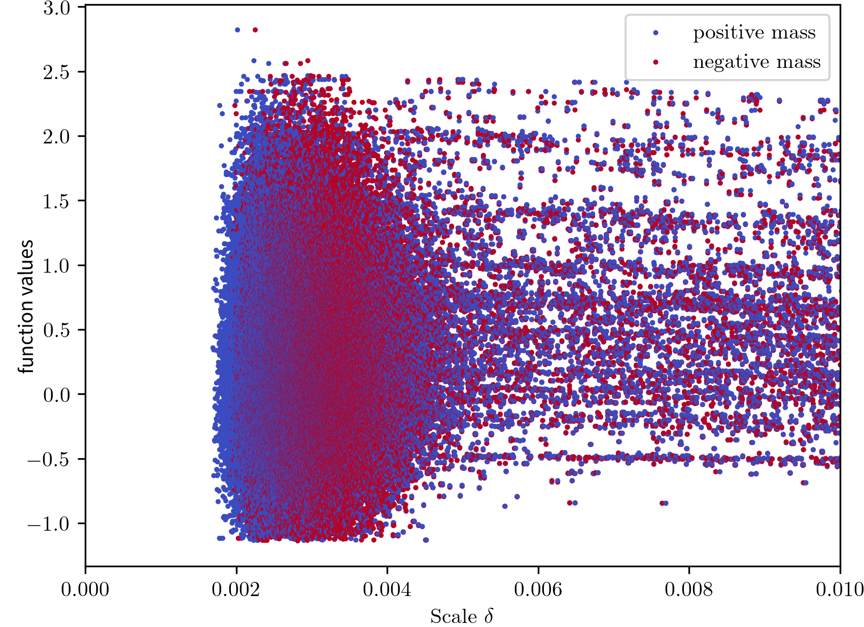
Here is a heuristic we apply to select a relevant rate . Since the dimension of the domain is known, we set to be a fixed fraction of the theoretical rate . This choice is motivated in the full version [1] and ensures that, up to a multiplicative constant, the rate cannot be improved for any (possibly deterministic) -sample of a -dimensional space. To determine a good multiplicative constant, we notice from Figure 7 that, when , the error of the estimators soars, due to the fact that and do not have the same topology. According to Theorem 3, the optimal scale is then given as the smallest value lying above that interval, that is: . Our rate is an estimate of this value. In order to compute it, we look at the topological changes of as increases. Since the measure is uniform and thus does not exhibit pathological local behaviors, the artifacts in the topological type of should all vanish roughly at the same scale, and slightly before . This phenomenon, suggested by the shape of the curves in Figure 7, is further illustrated in Figure 8(a), where we consider the Hilbert function signed barcode [18, 21] of : after an initial transition phase () during which a concentration of positive generators appears, followed then by a concentration of negative generators, the structure of the module stabilizes as these positive and negative generators cancel each other out. This is highlighted when summing the signed generators within the half-plane , or equivalently, when computing the pointwise dimension of , for ranging from to , as shown in Figure 8(b). Since the convexity radius is infinite in this case, we have for all , and so our heuristic to determine a suitable rate from a sample for some sufficiently large is:
-
1.
Compute the pointwise dimension of as in Figure 8(b) for a range of ;
-
2.
Identify the transition phase of ;
-
3.
Choose a scale past this phase, so that is constant;
-
4.
Define the rate for as .
In Figure 9, we observe that both rates and achieve good performance asymptotically, with a convergence rate that is at least of the order of . However, the asymptotic regime is reached earlier with than with – while, as we said, it is not reached with .
5.2.2 Estimating the combined functions
We now study the function and approximate the corresponding 3-parameter persistence module . For this we employ the estimator , where, for each sample size , the scale parameter is given by the same as in Section 5.2.1. Since computing the interleaving distance in this context is NP-hard [3], we use the matching distance [15] as a proxy, estimated via Monte Carlo with random lines in . The results are shown in Figure 10. Notably, the observed convergence rate matches that of the previous experiment in Figure 9(a), which suggests that the empirical convergence rate is independent of the number of parameters.

5.3 Brownian motion in 1-d (involving a Hölder function)
The Brownian motion is not Lipschitz continuous but almost surely almost everywhere -continuous for any modulus of continuity of the form , with and large enough [20, Corollaries 1.20 and 5.3]. Let be a realization of a standard Brownian motion, which can be approximated by a Rademacher random walk.
For each , we build a -sample in according to the uniform distribution, as shown in Figure 11 for several values of . Then, since our goal here is to illustrate Theorem 3, we assume we have access to the sampling error and so we use the estimator to approximate the target for various sample sizes . The corresponding results are shown in Figure 12. A regression analysis of the experimental data indicates that which aligns closely with the theoretical prediction from Theorem 3, stating that the interleaving distance between and should be at most .
5.4 Timings
In the following table we report the running times for some of our experiments. Only the first one involves our algorithm for computing a presentation of . For all computations we used an Intel® Core™ i9-12900K CPU (5.2 GHz max) equipped with 125 GB of RAM.
| Experiment | Estimator | #Params | #Points | Filt. size | Filt. time | Invariant time |
|---|---|---|---|---|---|---|
| 2 circles | 2 | 220 | 13,110 | 11.8 ms |
6.5 ms
(presentation) |
|
| Immune cells (single ) | 2 | 6172 | 24,370 | 864 ms |
50.3 ms
(Hilbert measure) |
|
|
Brownian
motion |
1 | 10,000 | 37,359 | 1.21 s |
5.4 ms
(barcode) |
References
- [1] Ethan André, Jingyi Li, David Loiseaux, and Steve Oudot. Estimating the persistent homology of -valued functions using function-geometric multifiltrations, 2025. arXiv:2412.04162.
- [2] Ulrich Bauer and Michael Lesnick. Induced matchings and the algebraic stability of persistence barcodes. Journal of Computational Geometry, 6, 2015. doi:10.20382/JOCG.V6I2A9.
- [3] Håvard Bakke Bjerkevik, Magnus Bakke Botnan, and Michael Kerber. Computing the interleaving distance is np-hard. Foundations of Computational Mathematics, 20(5):1237–1271, 2020. doi:10.1007/S10208-019-09442-Y.
- [4] Omer Bobrowski, Sayah Mukherjee, and Jonathan E. Taylor. Topological consistency via kernel estimation. Bernoulli, 23(1):288–328, 2017.
- [5] Magnus Bakke Botnan, Vadim Lebovici, and Steve Oudot. On rectangle-decomposable 2-parameter persistence modules. Discrete & Computational Geometry, pages 1–24, 2022.
- [6] Mathieu Carriere, Bertrand Michel, and Steve Oudot. Statistical analysis and parameter selection for mapper. Journal of Machine Learning Research, 19(12):1–39, 2018. URL: https://jmlr.org/papers/v19/17-291.html.
- [7] F. Chazal and S. Y. Oudot. Towards persistence-based reconstruction in Euclidean spaces. In Proc. 24th ACM Sympos. Comput. Geom., pages 232–241, 2008.
- [8] Frédéric Chazal, David Cohen-Steiner, Marc Glisse, Leonidas J Guibas, and Steve Y Oudot. Proximity of persistence modules and their diagrams. In Proceedings of the twenty-fifth annual symposium on Computational geometry, pages 237–246, 2009. doi:10.1145/1542362.1542407.
- [9] Frédéric Chazal, Vin De Silva, Marc Glisse, and Steve Oudot. The structure and stability of persistence modules, volume 10. Springer, 2016. doi:10.1007/978-3-319-42545-0.
- [10] Frédéric Chazal, Leonidas J Guibas, Steve Y Oudot, and Primoz Skraba. Scalar field analysis over point cloud data. Discrete & Computational Geometry, 46(4):743–775, 2011. doi:10.1007/S00454-011-9360-X.
- [11] Frédéric Chazal, Leonidas J Guibas, Steve Y Oudot, and Primoz Skraba. Persistence-based clustering in Riemannian manifolds. Journal of the ACM (JACM), 60(6):1–38, 2013. doi:10.1145/2535927.
- [12] Tamal K Dey, Jan Jendrysiak, and Michael Kerber. Decomposing multiparameter persistence modules. arXiv preprint, 2025. arXiv:2504.08119.
- [13] Allen Hatcher. Algebraic Topology. Cambridge Univ. Press, 2001. URL: http://www.math.cornell.edu/˜hatcher/.
- [14] Rafal Komendarczyk, Sushovan Majhi, and Will Tran. Topological stability and latschev-type reconstruction theorems for spaces of curvature bounded above. arXiv preprint, 2024. arXiv:2406.04259.
- [15] Claudia Landi. The rank invariant stability via interleavings. In Research in computational topology, pages 1–10. Springer, 2018.
- [16] Janko Latschev. Vietoris-Rips complexes of metric spaces near a closed Riemannian manifold. Archiv der Mathematik, 77(6):522–528, 2001.
- [17] David Loiseaux, Mathieu Carrière, and Andrew J. Blumberg. Multi-parameter Module Approximation: An efficient and interpretable invariant for multi-parameter persistence modules with guarantees. Journal of Applied and Computational Topology, 9(4):26, December 2025. doi:10.1007/s41468-025-00222-y.
- [18] David Loiseaux, Luis Scoccola, Mathieu Carrière, Magnus Bakke Botnan, and Steve Oudot. Stable Vectorization of Multiparameter Persistent Homology using Signed Barcodes as Measures. Advances in Neural Information Processing Systems, 36:68316–68342, December 2023.
- [19] Saunders Mac Lane. Categories for the working mathematician, volume 5. Springer Science & Business Media, 2013.
- [20] Peter Mörters and Yuval Peres. Brownian Motion, volume 30. Cambridge University Press, 2010.
- [21] Steve Oudot and Luis Scoccola. On the stability of multigraded Betti numbers and Hilbert functions. SIAM Journal on Applied Algebra and Geometry, 8(1):54–88, 2024. doi:10.1137/22M1489150.
- [22] Steve Oudot and Lukas Waas. A persistent version of Latschev’s theorem. In 42nd International Symposium on Computational Geometry (SoCG 2026), Leibniz International Proceedings in Informatics (LIPIcs), pages 82:1–82:17. Schloss Dagstuhl – Leibniz-Zentrum für Informatik, 2026. doi:10.4230/LIPIcs.SoCG.2026.82.
- [23] Alexander Rolle and Luis Scoccola. Stable and consistent density-based clustering via multiparameter persistence. Journal of Machine Learning Research, 25(258):1–74, 2024.
- [24] Oliver Vipond, Joshua A. Bull, Philip S. Macklin, Ulrike Tillmann, Christopher W. Pugh, Helen M. Byrne, and Heather A. Harrington. Multiparameter persistent homology landscapes identify immune cell spatial patterns in tumors. Proceedings of the National Academy of Sciences, 118(41):e2102166118, October 2021. doi:10/gpd543.