Computing the Bottleneck Distance Between Persistent Homology Transforms

Abstract
The Persistent Homology Transform (PHT) summarizes a shape in by collecting persistence diagrams obtained from linear height filtrations in all directions on . It enjoys strong theoretical guarantees, including continuity, stability, and injectivity. A natural way to compare two PHTs is to use the bottleneck distance between their diagrams as the direction varies. Prior work has either compared PHTs by sampling directions or, in 2D, computed the exact integral of bottleneck distance over all angles via a kinetic data structure. We improve the integral objective to in place of the earlier bound, where denotes the number of simplices. For the max objective, we give an expected-time algorithm in and an expected-time algorithm in .
Keywords and phrases:
Kinetic data structure, bottleneck distance, persistent homology transform, vineyardsFunding:
Michael Kerber: Supported by the Austrian Science Fund (FWF) 10.55776/P33765.Copyright and License:
![[Uncaptioned image]](x1.png) © Michael Kerber and Elena Xinyi Wang; licensed under Creative Commons License CC-BY 4.0
© Michael Kerber and Elena Xinyi Wang; licensed under Creative Commons License CC-BY 4.0
2012 ACM Subject Classification:
Mathematics of computing Algebraic topology ; Theory of computation Computational geometryEditors:
Hee-Kap Ahn, Michael Hoffmann, and Amir NayyeriSeries and Publisher:
 Leibniz International Proceedings in Informatics, Schloss Dagstuhl – Leibniz-Zentrum für Informatik
1 Introduction
Persistent homology captures the multiscale evolution of homology classes along a filtration induced by a real-valued function on a space. It has proved useful across fields such as materials science [9, 14], computational biology [12, 19], as well as machine learning [3, 13], providing robust descriptors for high-dimensional data. A persistence diagram is a concise multiset summary of persistent homology, recording the birth–death times of features. Similarity between objects is then assessed by comparing their diagrams, most commonly via the bottleneck distance. Computationally, this reduces to a minimum-bottleneck perfect matching on a bipartite graph with diagonal copies, and algorithms for this problem have been studied extensively in both theory and practice [2, 6, 10, 15, 16].
Since a single diagram depends on the chosen filter and may miss geometry, the Persistent Homology Transform (PHT) collects diagrams from all directions to retain fuller information [20]. It assigns to a shape in the collection of persistence diagrams obtained from linear height filtrations over all directions on . It possesses many desirable theoretical properties such as continuity, stability, and injectivity [5, 11, 20]. These properties make the PHT an effective topological descriptor for applications. However, unlike other directional-transform–based signatures such as the Euler Characteristic Transform, the PHT lacks efficient comparison algorithms, limiting its practical use. A natural way to compare PHTs is to sample directions and compute the bottleneck distance only at those angles. This inevitably leads to information loss. To integrate the bottleneck distance over the parameter domain (e.g., ), prior work by Munch, Wang, and Wenk introduced a kinetic “hourglass” approach that maintains matchings as the parameter moves. It computes this integral with an bound for data in [18]. In this work, we focus on the max variant, which we define as the supremum of the bottleneck distance over all directions.
Our Contributions.
We provide an expected-time algorithm to compute the max bottleneck distance between PHTs of shapes in and an expected-time algorithm in , where means the logarithmic factor is ingored. Additionally, we improve the computation of the integral distance from the previous bound to in .
For the max bottleneck distance, we use techniques from computational geometry and topology and inspired by the strategy of Bjerkevik and Kerber for computing the matching distance for two-parameter modules [1]. At a high level, the solution for 2D and 3D are similar. We first reformulate the problem as a decision problem: given a threshold , we determine whether the max bottleneck distance is at most . To solve this, we sweep the direction parameter around the sphere while maintaining the bottleneck matching between the two persistence diagrams. The key insight is that this matching changes only at discrete “events”: points where persistence diagrams change combinatorially or where edge weights cross the threshold . At each event, we update the matching using a single augmenting path search in the geometric bipartite graph, exploiting the fact that only local changes occur.
We then identify that the maximum bottleneck distance must occur at one of a finite set of candidate values, corresponding to critical points and intersections of the difference functions between simplices. While there are candidates in 2D and in 3D, we avoid exhaustive enumeration through a randomized incremental construction. We maintain a band containing the true maximum and iteratively refine it by processing simplices in random order, testing whether their associated candidates lie within the current band. The randomization ensures that we expect only refinements, reducing the expected complexity to in 2D and in 3D.
Outline.
We begin in Section 2 with a brief overview of persistent homology, persistence diagrams, and the PHT, and we formalize the problem. Section 3 presents our algorithm: first at a high level, then with full technical details. The improvement for the integral distance is shown in Section 4. Section 5 extends the approach to before concluding in Section 6.
2 Preliminary
2.1 Persistent homology
Persistent homology is a multi-scale summary of the connectivity of objects in a nested sequence of subspaces; see [7, 8] for an introduction. For the purposes of this section, we define a persistence diagram to be a finite collection of points with for all .
Given two persistence diagrams and , a partial matching is a bijection on a subset of the points and ; we denote this by . The cost of a partial matching is the maximum over the -norms of all pairs of matched points and the distance between the unmatched points to the diagonal:
| (1) |
and the bottleneck distance is defined as .
We can reduce finding the bottleneck distance between persistence diagrams to the problem of finding the bottleneck cost of a bipartite graph. Let and be two persistence diagrams given as finite lists of off-diagonal points. For any off-diagonal point , the orthogonal projection to the diagonal is . Let (resp. ) be the set of orthogonal projections of the points in (resp. ). Set and . We define the complete bipartite graph , where for and , the weight function c is given by
An example of the bipartite graph construction is shown in Figure 1. This graph can be used to compute the bottleneck distance of the input diagrams because of the following lemma.
Lemma 1 (Reduction Lemma [8]).
For the above construction of , .
2.2 Persistent homology transform
Let be a finite simplicial complex embedded in . For any direction , the height function is defined by . The lower-star filtration induced on the abstract complex is given by:
and the sublevelset at height is the full subcomplex induced by vertices . Filtering by produces a persistence diagram . We focus on for , and for .
2.3 Maximum bottleneck distance
In this work, we are interested in comparing two finite embedded simplicial complexes, , or , by comparing their PHTs. We define the maximum bottleneck distance between and to be:
This distance is a variant of a similar integral distance that has been studied previously by Munch, Wang, and Wenk [18]:
Both and inherit stability from the bottleneck distance. However, they differ from a computational perspective. Computing requires full knowledge of the whole domain, which is inevitably expensive. Our metric seeks the maximum value, which allows us to reformulate the problem as finding the supremum over a finite set of candidate values rather than tracking the bottleneck distance continuously.
A key property that makes our algorithmic approach feasible is that the bottleneck distance function is Lipschitz continuous, which is a direct consequence of the stability of the bottleneck distance (see the full version for a complete proof):
Lemma 2.
Let denote the bottleneck distance between persistence diagrams. Then the function is Lipschitz continuous with constant , where and .
3 Computing in
Our setup in this section is as follows: we are given two geometric simplicial complexes , in with at most simplices each. The goal is to compute : we first introduce the necessary notation, then give a high-level overview, and finally present the technical details.
3.1 Events
For each simplex , we define an insertion curve . These curves record the height at which each simplex enters the sublevel-set filtration induced by direction . Explicitly, if the -simplex has vertices , its insertion curve is
Each is a piecewise-trigonometric function on .
There are at most such curves. We now define difference curves that capture both matched and unmatched contributions to the bottleneck distance. For distinct simplices :
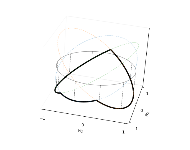
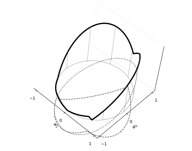
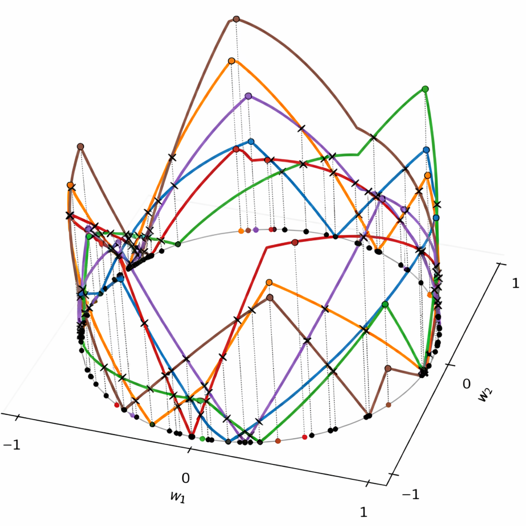
These are real-valued functions on ; geometrically, one can picture their graphs as curves in . The factor of corresponds to the contribution of unmatched points to the bottleneck distance, see Equation 1. There are such curves for . We call the vertex achieving the active vertex of at . As varies, the active vertex changes at discrete directions where two vertices achieve the same height. Within any interval where the active vertices remain fixed, the difference curve simplifies to either (for different complexes) or (for same complex), which is a simple trigonometric function. See Figure 2 for an example. The insertion and difference curves are both well-behaved. See Figure 3 for an example.
Lemma 3.
Each difference curve crosses any horizontal line at most times as varies over . Since there are difference curves in total, this yields crossings with any horizontal line. In particular, there are insertion-curve intersections, as these correspond to difference curves crossing the line .
The bound on insertion-curve intersections follows immediately since we have curves total, giving at most pairwise intersections. For threshold crossings, each difference curve is piecewise trigonometric with pieces (as simplices in have at most 3 vertices), and crosses any threshold at most times. With pairs total, this yields threshold crossings. The detailed geometric analysis is in the full version.
In each direction , the bottleneck distance is realized by the value of a difference curve . When this maximum is unique in a neighborhood of , the continuity of the bottleneck function ensures that the same curve or persistence value realizes the bottleneck distance in an -neighborhood. We call the points in where the realizing curve or value changes locally events, and the values attains at events are the candidate values.
Theorem 4 (Events for in ).
The direction attaining occurs at either
-
1.
a local maximum of a difference curve , or
-
2.
an intersection of two difference curves. See Figure 3 for an illustration.
Proof.
Let be the direction that attains . By Lemma 2, if the bottleneck distance at is realized by a unique difference curve in a neighborhood, then must be a local maximum of that difference curve, giving case (1). This includes both matched pairs (when ) and unmatched point persistence (when are from the same complex). Otherwise, at least two curves achieve the same maximum value at , giving case (2). Note that intersections of insertion curves (where the persistence diagram changes combinatorially) form a special case of (2), as when two insertion curves from the same complex coincide, all difference curves of the form and are equal.
Remark 5.
When we refer to “intersections” of difference curves, we mean isolated transverse crossings, not intervals of coincidence. Endpoints of overlaps also count as intersections, since the realizing curve may change at those boundaries.
(a)
(b)
(c)
Corollary 6.
There are candidate values where may be attained.
Proof.
There are difference curves: from pairs , plus from pairs within the same complex. Each has local maxima (see the full version for the explicit bound), contributing type-(1) candidates. For type-(2) candidates, each pair of difference curves intersects at heights, giving intersections total. Thus the total number of candidates is .
Remark 7.
When simplices share vertices, their difference curves may partially coincide. For instance, if share vertex and share vertex , then and coincide in regions where and are simultaneously active. Despite these overlaps, each difference curve retains a unique identity at the combinatorial level through its defining simplex pair. In particular, our candidate enumeration remains valid: if the maximum bottleneck distance is achieved at direction , then at least one combinatorially distinct difference curve must realize this maximum, and this curve’s critical points and intersections are in our candidate set. The full technical detail is in the full version.
3.2 Overview of the algorithm
We describe the high-level structure of our algorithm next. On this level, our approach is similar to the algorithm of Bjerkevik and Kerber to compute the matching distance [1]. However, the approaches differ in the technical realization of the predicates which are described in the subsequent subsections.
Decision procedure.
Given a threshold , we decide whether by sweeping around and maintaining a bottleneck matching. As rotates, we update the persistence diagrams at insertion-curve intersections and perform single augmenting-path updates whenever an edge weight crosses the threshold. This decision procedure runs in time.
Basic algorithm.
By Theorem 4, is attained at one of candidate values corresponding to intersections of difference curves and their local maxima. These candidates can be enumerated and sorted in time. Combined with binary search using our decision procedure, this yields an algorithm.
Improved algorithm via band refinement.
By Theorem 4, there are total candidates where could be attained. To achieve time, we avoid enumerating all candidates.
We call a candidate an -candidate if it arises from a difference curve for some (when ), from for some (when ), or from for some in the same complex as .
We maintain a height band satisfying and . We process simplices from both complexes in random order. For each simplex , we apply:
-
1.
Existence predicate: Tests if any -candidate lies in in time. If no candidate exists in the band, we skip to the next simplex.
-
2.
Band-refinement predicate: If the existence test is positive, we enumerate all -candidates in the band and refine via binary search in time.
The resulting total running time is , where is the number of band-refinement calls. As we will show, processing the simplices in a random order ensures , yielding expected time .
3.3 Decision problem
We now describe how to decide whether for a given threshold . The key idea is to sweep the direction around and check if the bottleneck distance ever exceeds .
By Lemma 1, at each direction , the bottleneck distance equals the cost of a minimum-bottleneck matching in a bipartite graph constructed from the two persistence diagrams and with diagonal copies. Define the subgraph to contain only those edges of whose weights are . Then if and only if admits a perfect matching.
Our strategy is to maintain a perfect matching in as sweeps from to . If at any point no perfect matching exists, we conclude ; otherwise, if the sweep completes with a valid matching at every direction, then .
Sweep algorithm.
We initialize at by computing a perfect matching in using Hopcroft-Karp in [15]; if none exists, .
As increases from to , the bipartite graph changes only at discrete events:
-
Diagram changes: At intersections of insertion curves, points move to or from the diagonal in the persistence diagrams, updating the bipartite graph structure.
-
Threshold crossings: When a difference curve crosses the threshold , the corresponding edge enters or leaves .
Maintaining the matching.
A matching is maintained across the sweep. At each event:
-
If a new edge enters (weight decreases below ), remains valid.
-
If an edge leaves (weight exceeds ) and is not in , then remains valid.
-
If an edge becomes invalid, Hall’s theorem guarantees that a new perfect matching exists if and only if there is an augmenting path from the newly exposed vertices. We search for such a path in time using the geometric structure [10]. If found, we augment along this path to restore a perfect matching. If no augmenting path exists, then has no perfect matching, so at this , implying .
At diagram change events (insertion curve intersections), we update the persistence diagrams using the vineyard algorithm [4]. When two insertion curves and from the same complex intersect, the relative order of exactly two simplices changes in the filtration. Following Bjerkevik and Kerber [1], this corresponds to a single transposition in the barcode pairing, which can be updated in time.
If the sweep completes with a valid perfect matching at every , then .
Lemma 8.
The decision procedure runs in time.
Proof.
At each event, we either update the diagram structure in time (vineyard update for insertion curve intersections) or search for a single augmenting path in time (for threshold crossings). With total events from Lemma 3, the total time is .
3.4 Candidate pruning via band refinement
Recall that we have total candidates where may be attained. To find efficiently, we maintain a height band containing and iteratively shrink it by processing simplices from both complexes in random order.
We distinguish between two types of intersections between difference curves. Intra-intersections occur when two difference curves share a common simplex: either and sharing simplex , or and sharing simplex . Inter-intersections occur when and meet with all four simplices distinct: and .
Pre-refinement.
Before processing individual simplices, we refine the band to exclude certain events from its interior: let be the set containing all local maxima of difference curves for all pairs (including both different-complex and same-complex pairs), all intra- intersections where for some and distinct , and all intra- intersections where for distinct .
Since there are difference curves, each with local maxima, we have maxima total. For intra-intersections, each of the simplices in contributes pairs of curves that could intersect, with intersection points each, giving intra- intersections. Similarly for intra- intersections. Thus .
We binary search with the decision procedure to find the largest value in below and the smallest at or above it, setting these as and . The resulting band contains no intra-events in its interior. This takes time.
3.4.1 Predicate 1: Existence test
After pre-refinement, we process simplices to detect inter-intersections.
Lemma 9.
For fixed , determining whether any inter-intersection involving lies in takes time.
Proof.
We seek intersections of the form where . For each , we define the red curves as all curves involving simplex , and the blue curves as all curves involving simplex . (See Figure 2 for the geometric setting; the red and blue curves are real-valued functions on , and we detect their intersection as real-valued crossing events while sweeping around .)
The key insight from pre-refinement is that within the band , no two red curves can intersect (these would be intra- intersections), and no two blue curves can intersect (these would be intra- intersections).
Each difference curve consists of trigonometric pieces, switching between different expressions at directions where the active vertex changes. Since simplices in have at most 3 vertices, there are such transition points. When we clip to the band , each curve crosses the boundary at points, subdividing into monotone arcs within the band.
We apply the standard Bentley-Ottmann sweep-line algorithm to all arcs. Since red arcs do not intersect each other and blue arcs do not intersect each other (by pre-refinement), any intersection must be between a red and blue arc. We terminate immediately upon detecting the first such intersection. This takes time per choice of . Testing all choices of takes total time for fixed .
3.4.2 Predicate 2: Band refinement
When the existence test detects an inter-intersection, we must enumerate all candidates involving to refine the band.
Lemma 10.
When an inter-intersection involving is detected, we can enumerate all -candidates in and compute a refined band with no -candidates in its interior in time.
Proof.
After pre-refinement, only inter-intersections remain in the band’s interior. For simplex , there are such intersections (choosing with choices each). We enumerate these candidates, sort them, and refine the band using binary search with the decision procedure, taking time.
Theorem 11.
After global pre-refinement, processing each simplex takes total time, where is the indicator function of the existence test.
Proof.
3.4.3 Randomized analysis
Theorem 12.
Processing simplices from both and in uniformly random order yields refinements, where counts positive existence tests.
Proof.
For each simplex , define as the smallest -candidate that is and as the largest -candidate that is . Since is realized by at least one candidate, for some simplex we have . Every interval contains , so our maintained band always has the form for some processed simplices .
When processing simplices in random order, we obtain random permutations of the sequences and . Simplex passes the existence test and the refinement is triggered if and only if there exists an -candidate in the current band. This occurs when is smaller than all previously seen values (making it a left-to-right minimum), or is larger than all previously seen values (making it a left-to-right maximum).
Indeed, if is not a minimum, then some previously processed satisfies , so the band’s upper bound is already at most , excluding all -candidates with value . Likewise, if is not a maximum, the band’s lower bound already exceeds , excluding all -candidates with value . Thus, when neither nor improves the band boundaries, every -candidate lies outside , and none can fall in the current band.
By a classical result on random permutations [17]: in a uniformly random ordering of distinct values, the -th element is a left-to-right minimum with probability (being the smallest of the first elements). By linearity of expectation, the expected number of left-to-right minima is . The same bound holds for maxima. Therefore, the expected number of refinements is at most the expected number of minima in plus the expected number of maxima in , giving .
Corollary 13.
The candidate pruning algorithm runs in expected time
Proof.
We process simplices from both complexes. Each requires an existence test. In expectation, only trigger the band refinement. The refinement cost dominates, giving expected time.
4 Computing in
Our framework also improves the computation of the integral bottleneck distance from the previous bound [18] to .
The integral requires maintaining the bottleneck matching as sweeps around . As varies, the bottleneck distance changes only at the difference curve intersection events identified in Section 3. At each event, we update the matching in time via an augmenting path search to identify which difference curve realizes the new bottleneck. Between consecutive events at angles and , the bottleneck distance is given by a single difference curve that can be integrated analytically.
Thus the integral distance can be computed in total time: events, each requiring processing. This improves upon the hourglass data structure approach of [18], which maintained two kinetic heaps and required time.
5 Computing in
We now consider embedded complexes in . Directions range over the sphere , difference curves become surfaces, and intersections occur along curves rather than at points. The algorithm follows the same framework as 2D, but requires traversing an arrangement on via an Euler tour rather than sweeping a circle. This yields expected complexity .
5.1 Events
Let be finite simplicial complexes with at most simplices each. For each simplex , , the insertion surface is:
Each is the upper envelope of at most 4 trigonometric forms on . The loci where the maximizing vertex changes are great circles .
For distinct simplices , the difference surface is a real-valued function on :
Within each region where the active vertices are fixed, simplifies to for active vertices and . Two difference surfaces and intersect along curves on where .
Lemma 14.
For simplicial complexes in :
-
1.
Each pair of insertion surfaces intersects along great circle arcs on .
-
2.
Each pair of difference surfaces intersects along great circle arcs on .
-
3.
Each intersection curve between difference surfaces has local maxima.
-
4.
Each difference surface crosses any threshold along curves on .
The proof follows from the piecewise structure: since simplices in have at most 4 vertices, each insertion surface has regions of fixed active vertex. Within each region, the surfaces are trigonometric forms and their intersections are great circles. The detailed geometric analysis is in the full version.
Theorem 15 (Events for in ).
The direction attaining occurs at one of:
-
1.
A local maximum of a difference surface
-
2.
A local maximum along an intersection curve on where two difference surfaces meet
-
3.
A triple intersection point where three difference surfaces meet
Proof.
The bottleneck distance function is continuous on . At any where is attained, consider the difference surfaces achieving the maximum value .
If a unique surface achieves this maximum in a neighborhood of , then by continuity, must be a local maximum of that surface (case 1). This covers both matched pairs and unmatched persistence. If exactly two surfaces achieve the maximum at but no other surface does so nearby, then lies on their intersection curve on . Since is locally determined by these two surfaces along the curve, must be a local maximum along this curve (case 2). If three or more surfaces achieve the maximum at , then generically three surfaces meet at isolated points, giving case 3.
Corollary 16.
There are candidate values where may be attained.
Proof.
We count candidates by type. Type 1 has difference surfaces (including both between-complex and within-complex pairs), each having maxima, contributing candidates. Type 2 consists of pairs with maxima per intersection curve, giving candidates. Type 3 is triple intersection points. This gives us the total of candidates.
5.2 Overview of algorithm
Decision procedure.
Given threshold , we decide whether by traversing an arrangement on . Similar to the 2D case, we track two types of events:
-
Diagram changes: intersection curves between insertion surfaces where the persistence diagrams change combinatorially;
-
Threshold crossings: curves on where difference surfaces cross the threshold .
Overlaying these curves yields an arrangement of complexity on . We traverse the dual of this arrangement via an Euler tour by traversing each edge twice, maintaining a bottleneck matching throughout. Each diagram change requires time to update the barcode pairing using the vineyard algorithm, while each threshold crossing may require time for augmenting path search. The total complexity is .
Improved algorithm via band refinement.
We maintain a band containing and process simplices in random order. For each simplex :
-
1.
Existence predicate: Test if any -candidate lies in the band. Following the approach from 2D adapted to surfaces: for fixed and , consider the surface . For each , compute intersection curves with all surfaces. Within the band, these curves form disjoint arcs on (no intra- intersections after pre-refinement). Similarly get disjoint arcs from surfaces involving . Check for red-blue intersections in time. Testing all combinations takes .
-
2.
Band refinement: If positive, enumerate all -candidates in the band: triple intersections, curve maxima, surface maxima. Then refine via binary search in time.
Using the same randomization analysis as 2D, we expect refinements. This results in total expected complexity of .
5.3 Decision problem
Given threshold , we decide whether by constructing and traversing an arrangement on . Unlike the 2D case where we sweep around a circle, here we must systematically explore the entire sphere.
We first construct an arrangement on consisting of:
-
curves from insertion surface intersections (where persistence diagrams change)
-
curves where difference surfaces equal (threshold crossings)
Each insertion surface is piecewise trigonometric with pieces, so pairs intersect along curves each. Similarly, each difference surface crosses the threshold along curves. The overlay of all these curves forms an arrangement with vertices, edges, and faces.
Theorem 17.
Whether can be decided in time.
Proof.
We construct the arrangement and compute an Euler tour of its dual graph, treated as a planar graph embedded on . The tour visits each edge twice, once in each direction.
Starting from an arbitrary face with a perfect matching in , we traverse the tour and maintain the matching throughout. At insertion curve crossings where the persistence diagram changes, we update the barcode pairing via a single transposition in time using the vineyard algorithm. At threshold crossings where an edge weight exceeds , we search for an augmenting path in time. If no augmenting path exists, we conclude and terminate. If the tour completes with valid matchings maintained throughout, then for all , hence .
The arrangement has edges in total. The diagram changes contribute total time at each, while the threshold crossings contribute at each. However, the bottleneck arises from traversing all edges of the arrangement, where at each edge crossing we may need to update the matching. Since each edge crossing potentially requires time for augmenting path search, the total complexity is .
5.4 Candidate pruning via band refinement and complexity analysis
As in the 2D case, we maintain a band containing and process simplices in random order. We first apply a pre-refinement to exclude all intra-events from the band.
Pre-refinement.
Before processing individual simplices, we refine the band to exclude all intra-events from its interior. We call a triple intersection point an intra-event if any two of the six involved simplices are equal. Let be the set containing all local maxima of difference surfaces, all local maxima along surface intersection curves, and all intra-event triple intersections. Since there are ways to choose 5 distinct simplices and ways to make two of them equal, we have . We use binary search with the decision procedure to find the largest value in that is (setting ) and the smallest value in that is (setting ), yielding the band that contains but excludes all values of from its interior. This takes time.
Lemma 18.
For fixed , we can test whether any inter-intersection involving lies in the band in time.
Proof.
Fix and , giving the difference surface . We seek triple intersection points of the form where and , with the intersection value lying in .
For fixed , compute the intersection curves between and all surfaces for . Each pair of surfaces intersects along great circle arcs on where . We obtain intersection curves on .
The crucial observation is that when we restrict to the band , these curves become disjoint arcs. Any intersection between curves and would yield a triple point where . This is an intra-event (two surfaces share ), excluded from the band’s interior via pre-refinement.
Similarly, for fixed , the intersection curves between and all surfaces yield another set of disjoint arcs within the band. We now have two collections of arcs on the restricted domain of : the “red” arcs from -surfaces and the “blue” arcs from -surfaces. A red-blue intersection corresponds to a triple point , which is an inter-intersection involving .
To detect red-blue intersections, we apply stereographic projection from the north pole of to map the band region to a planar domain and use a sweep-line algorithm. As shown in the full version, the projection preserves the disjointness of red and blue arc families while mapping great circle arcs to well-behaved curves (circles and lines) that intersect times. The sweep-line algorithm thus detects all red-blue intersections in time.
Iterating over all choices of , , and gives total complexity .
Lemma 19.
When the existence test is positive for simplex , we can enumerate all candidates involving that lie in .
Proof.
For each , the pre-refinement step excludes the local maxima of difference surfaces and local maxima of intersection curves. We only need to consider triple intersection points : with choices each for , and intersection points per triple, we get candidates. Total enumeration takes time. Binary search with the decision procedure then refines the band in time.
Theorem 20 (Total complexity in 3D).
The algorithm runs in expected time .
Proof.
We process simplices from both complexes. For each simplex , we perform the existence test in time. If positive, we enumerate and refine in time. We expect refinements using the same analysis as in 2D. The total expected complexity is therefore .
6 Conclusion
We have presented the first algorithms for computing the maximum bottleneck distance between Persistent Homology Transforms, achieving expected time complexity of in and in . As a byproduct, our framework also improves the integral bottleneck distance computation from to in 2D. Using similar techniques, the integral version in can be computed in time by maintaining matchings across all events, though we leave the technical details for future work.
Our adaptation of the framework introduced by Bjerkevik and Kerber [1] reveals a broader principle: directional transforms that vary continuously over parameter spaces can often be optimized through event-driven algorithms and randomized candidate pruning. This suggests potential applications beyond the PHT to other parametric problems in computational topology, such as the Euler Characteristic Transform or persistence-based shape signatures.
From a practical perspective, the cubic complexity in 2D makes exact PHT comparison feasible for moderate-sized datasets, potentially enabling new applications in shape matching and retrieval where sampling-based approximations were previously necessary. However, significant challenges remain: extending to the Wasserstein distance would require fundamentally different techniques due to its non-combinatorial nature, and handling higher-dimensional ambient spaces faces steep complexity barriers.
References
- [1] Havard Bakke Bjerkevik and Michael Kerber. Asymptotic improvements on the exact matching distance for -parameter persistence. Journal of Computational Geometry, 14(1):309–342, December 2023. doi:10.20382/jocg.v14i1a12.
- [2] Sergio Cabello, Siu-Wing Cheng, Otfried Cheong, and Christian Knauer. Geometric Matching and Bottleneck Problems. In Wolfgang Mulzer and Jeff M. Phillips, editors, 40th International Symposium on Computational Geometry (SoCG 2024), volume 293 of Leibniz International Proceedings in Informatics (LIPIcs), pages 31:1–31:15, Dagstuhl, Germany, 2024. Schloss Dagstuhl – Leibniz-Zentrum für Informatik. doi:10.4230/LIPIcs.SoCG.2024.31.
- [3] Mathieu Carrière, Frederic Chazal, Yuichi Ike, Theo Lacombe, Martin Royer, and Yuhei Umeda. Perslay: A neural network layer for persistence diagrams and new graph topological signatures. In Silvia Chiappa and Roberto Calandra, editors, Proceedings of the Twenty Third International Conference on Artificial Intelligence and Statistics, volume 108 of Proceedings of Machine Learning Research, pages 2786–2796. PMLR, 26–28 August 2020. URL: https://proceedings.mlr.press/v108/carriere20a.html.
- [4] David Cohen-Steiner, Herbert Edelsbrunner, and Dmitriy Morozov. Vines and vineyards by updating persistence in linear time. In Proceedings of the Twenty-Second Annual Symposium on Computational Geometry, SCG ’06, pages 119–126, New York, NY, USA, 2006. Association for Computing Machinery. doi:10.1145/1137856.1137877.
- [5] Justin Curry, Sayan Mukherjee, and Katharine Turner. How many directions determine a shape and other sufficiency results for two topological transforms. Transactions of the American Mathematical Society, Series B, 2018.
- [6] Tamal K. Dey and Cheng Xin. Computing Bottleneck Distance for 2-D Interval Decomposable Modules. In Bettina Speckmann and Csaba D. Tóth, editors, 34th International Symposium on Computational Geometry (SoCG 2018), volume 99 of Leibniz International Proceedings in Informatics (LIPIcs), pages 32:1–32:15, Dagstuhl, Germany, 2018. Schloss Dagstuhl – Leibniz-Zentrum für Informatik. doi:10.4230/LIPIcs.SoCG.2018.32.
- [7] Tamal Krishna Dey and Yusu Wang. Computational Topology for Data Analysis. Cambridge University Press, 1 edition, 2017. arXiv:1708.09359v2.
- [8] Herbert Edelsbrunner and John Harer. Computational Topology - an Introduction. American Mathematical Society, 2010.
- [9] Herbert Edelsbrunner and Teresa Heiss. Merge trees of periodic filtrations, 2024. doi:10.48550/arXiv.2408.16575.
- [10] Alon Efrat, Alon Itai, and Matthew J. Katz. Geometry helps in bottleneck matching and related problems. Algorithmica, 31(1):1–28, September 2001. doi:10.1007/s00453-001-0016-8.
- [11] Robert Ghrist, Rachel Levanger, and Huy Mai. Persistent homology and Euler integral transforms. Journal of Applied and Computational Topology, 2(1):55–60, October 2018. doi:10.1007/s41468-018-0017-1.
- [12] Chad Giusti, Eva Pastalkova, Carina Curto, and Vladimir Itskov. Clique topology reveals intrinsic geometric structure in neural correlations. Proceedings of the National Academy of Sciences, 112(44):13455–13460, 2015. doi:10.1073/pnas.1506407112.
- [13] Felix Hensel, Michael Moor, and Bastian Rieck. A survey of topological machine learning methods. Frontiers in Artificial Intelligence, Volume 4 - 2021, 2021. doi:10.3389/frai.2021.681108.
- [14] Yasuaki Hiraoka, Takenobu Nakamura, Akihiko Hirata, Emerson G. Escolar, Kaname Matsue, and Yasumasa Nishiura. Hierarchical structures of amorphous solids characterized by persistent homology. Proceedings of the National Academy of Sciences, 113(26):7035–7040, 2016. doi:10.1073/pnas.1520877113.
- [15] John E. Hopcroft and Richard M. Karp. An algorithm for maximum matchings in bipartite graphs. SIAM J. Comput., 2(4):225–231, December 1973. doi:10.1137/0202019.
- [16] Michael Kerber, Dmitriy Morozov, and Arnur Nigmetov. Geometry helps to compare persistence diagrams. ACM J. Exp. Algorithmics, 22, September 2017. doi:10.1145/3064175.
- [17] Donald E. Knuth. The Art of Computer Programming, Volume 3: Sorting and Searching. Addison-Wesley, 2nd edition, 1998. Section 5.1.1.
- [18] Elizabeth Munch, Elena Xinyi Wang, and Carola Wenk. The kinetic hourglass data structure for computing the bottleneck distance of dynamic data, 2025. doi:10.48550/arXiv.2505.04048.
- [19] Michael W. Reimann, Max Nolte, Martina Scolamiero, Katharine Turner, Rodrigo Perin, Giuseppe Chindemi, Paweł Dłotko, Ran Levi, Kathryn Hess, and Henry Markram. Cliques of neurons bound into cavities provide a missing link between structure and function. Frontiers in Computational Neuroscience, Volume 11 - 2017, 2017. doi:10.3389/fncom.2017.00048.
- [20] Katharine Turner, Sayan Mukherjee, and Doug M. Boyer. Persistent homology transform for modeling shapes and surfaces. Information and Inference: A Journal of the IMA, 3(4):310–344, December 2014. doi:10.1093/imaiai/iau011.