Non-Dissective Coverings by Planks

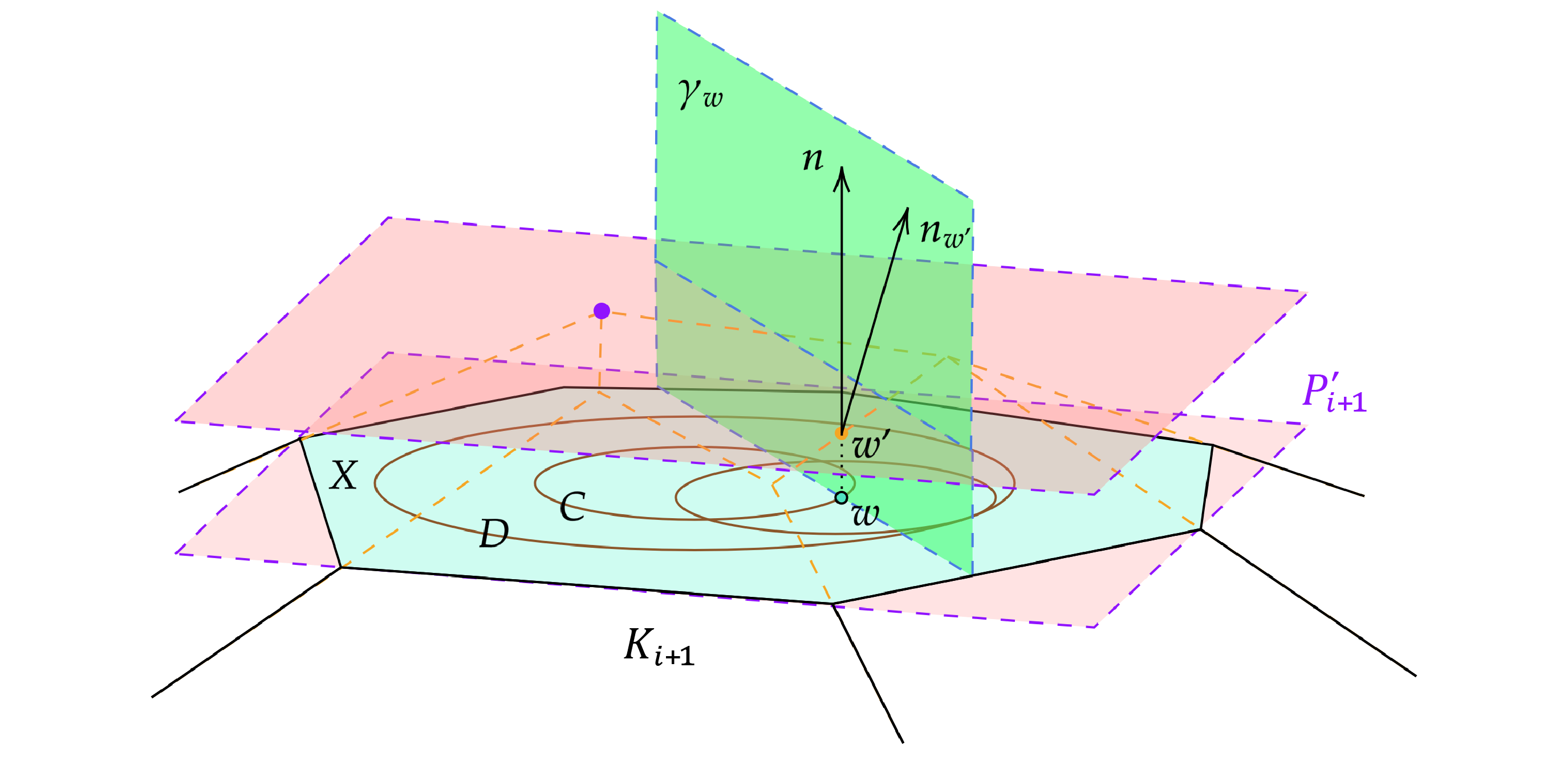
Let $n$ stand for the normal vector to ${\pi }^L$. For any point $w$ in $X$, we denote by $w^{\prime }$ the point on the boundary of $K_i$ that is obtained from $w$ by translating it parallel to $n$ inside $P_{i+1}^{\prime }$. Note that $w^{\prime }$ and $w$ are at most $ϵ$ apart.

Let us show that $X$ does not contain a disk $D$ of radius $10{ϵ}^{1/3}$. See Figure 1. Assume the contrary, and let $v$ be the center of such a disk $D$.

Consider the circle $C$ in ${\pi }^L$, concentric to $D$ and of radius $5{ϵ}^{1/3}$. Take a point $w\in C$. Consider the normal vector $n_{w^{\prime }}$ of a supporting plane for $K_i$ at $w^{\prime }$, whose choice we explain below. If $w^{\prime }$ lies on the boundary of, potentially, several planks $P_j^{\prime }$ with $j\le i$, then take a supporting hyperplane of one of these planks $P_j^{\prime }$. Otherwise, $w^{\prime }$ must lie on the boundary of the initial ball $B^3$, and then we simply take the unique supporting plane to the ball at $w^{\prime }$.

Consider the intersection $Q$ of $K_i\cap P_{i+1}^{\prime }$ with the plane ${\gamma }_w$ spanned by $n$ and $n_{w^{\prime }}$ and passing through $w$. By our assumption, $X$ contains a disk of radius $5{ϵ}^{1/3}$ centered at $w$. Thus, $Q$ is a convex set of height at most $ϵ$ and with the “base” being a straight line segment orthogonal to $n$ that passes through $w$ and has length at least $5{ϵ}^{1/3}$ in each direction from $w$. Thus, the angle between $n$ and $n_{w^{\prime }}$ is at most ${ϵ}^{2/3}$: otherwise, the supporting line at $w^{\prime }$ corresponding to $n_{w^{\prime }}$ will hit the base segment at distance at most from $w$, which is a contradiction. See Figure 2.

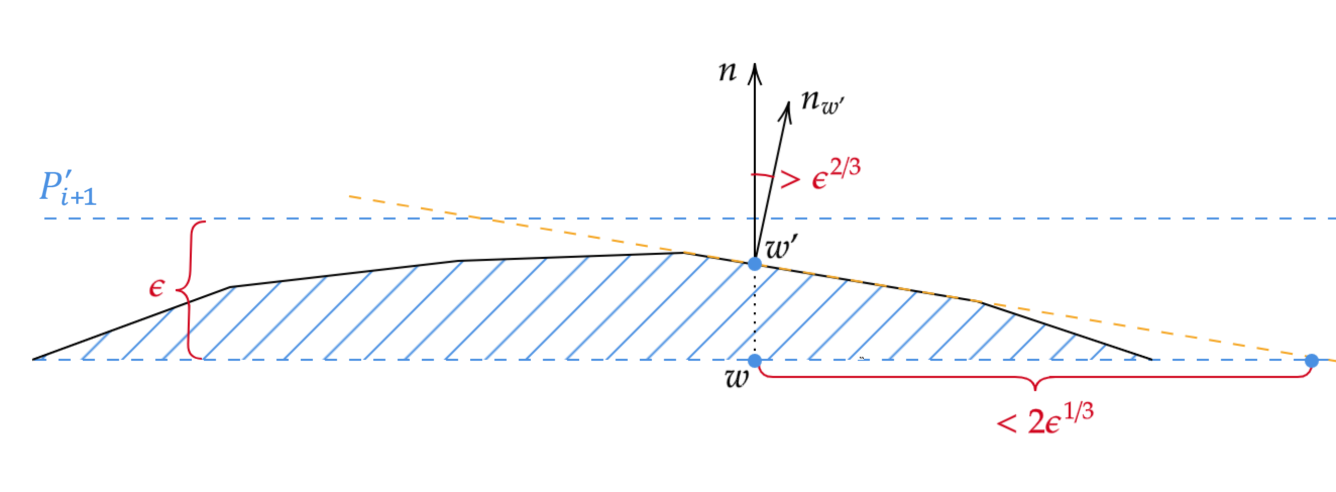
We conclude that $n_{w^{\prime }}$ has angle at most ${ϵ}^{2/3}$ with $n$ for any $w\in C$. Since the angle between the normal vectors of any two planks is at least $10{ϵ}^{2/3}$, $n_{w^{\prime }}$ cannot be a normal vector to any other plank. Running the same argument for each point $w\in C$, we conclude that the set $C^{\prime }:=\{w^{\prime }:w\in C\}$ lies on the boundary of $B^3$. But then the angle between the normal vectors at two points of $C^{\prime }$ corresponding to the opposite points of $C$ is $\mathrm{\Omega }(\mathrm{diam}(C))=\mathrm{\Omega }({ϵ}^{1/3})$, a contradiction with the fact that each of them has angle at most ${ϵ}^{2/3}$ with $n$. $◀$

We start by verifying the first inclusion. Let $v$ be any point of $B(K_{i-1}\setminus P_i^{\prime })$. By definition, there exists $w\in K_{i-1}\setminus P_i^{\prime }$ with $\Vert v-w\Vert \le 1.$ Thus, $v$ also belongs to $B(K_{i-1})$. We only have to argue that $v$ does not lie inside the half-space ${\mathrm{\Pi }}_i.$ If it did, by property 2 above, it would be farther away than $1$ from the lower boundary plane of $P_i^{\prime }$, which separates $K_{i-1}\setminus P_i^{\prime }$ from $v$. This would contradict our assumption that $v\in B(K_{i-1}\setminus P_i^{\prime }).$

The second inclusion holds since $P_i^{\prime \prime }\subset {\mathrm{\Pi }}_i.$ $◀$

Recall that, according to our conventions, the direction of the positive $z$-axis of the coordinate system coincides with the vector $n$. At the beginning, we fixed a vertical direction $n$, but in the sequel we will also use the following simple fact in other scenarios.

Now we quickly outline our proof strategy for the upper bound in Theorem 4. Recall that we selected a “dense” subset of almost parallel directions, in terms of two constants $\alpha$ and $\beta$. Our first and main goal is to bound from below the volume of the parallel body $B(K_j)$ of the part of $B$ that we cover with the first $j$ planks corresponding to the chosen directions. To get this lower bound, we will have two cases to consider, and the parameter $\alpha$ is chosen to balance the bound in the two cases. We cover a substantial part of $K_0=B^3$ using these planks, and remove them. This constitutes the first stage of our covering algorithm.

At the second stage, we repeat the same procedure. This time, in the remaining set of directions we find a “dense” subset (using the same $\alpha$), and we use the corresponding almost parallel planks to cover the remaining part of the ball. While at stage 1, we started with $K_0=B^3,$ at stage 2 we start where we left off at stage 1. That is, our new initial body $K_0^{(2)}$ will be identical to the last $K_j$ at stage 1. Again, we bound from below the volumes of the parallel bodies of the new shrinking sequence

of uncovered bodies. Because of our choice of parameters, it is guaranteed that after performing this procedure a bounded number of times, at some stage we reach a point where (2) holds. At this point, we can be sure that $B^3$ is entirely covered.

Apply Proposition 7 with $K_0=B^3$ to obtain a ball $U\subset B(K_0)$ of unit radius that touches the boundary of $B(K_0)$ at its highest point in the vertical direction $n$. Let $\mathrm{\ell }$ be the vertical line passing through the center of $U$ (which is the highest point of $B^3$).

We distinguish two cases.

Case A:

There is a set of indices $A\subset \{1,\mathrm{\dots },m\}$ with $|A|\ge m/2$ such that for any $i\in A,$ the intersection of $\mathrm{\ell }$ with $B(K_i)$ is at least $ϵ/2$ shorter than the intersection of $\mathrm{\ell }$ with $B(K_{i-1})$.

Case B:

There is a set of indices $Z\subset \{1,\mathrm{\dots },m\}$ with $|Z|\ge m/2$ such that for any $i\in Z$, the intersection of $\mathrm{\ell }$ with $B(K_i)$ is less than $ϵ/2$ shorter than the intersection of $\mathrm{\ell }$ with $B(K_{i-1})$.

In Case A, we start our argument as follows. To simplify the notation, assume that $m\in A$. Suppose that the center of $U$ is inside $B(K_m)$ and we have $mϵ=o(1)$. Using Proposition 6, we obtain that

Since $U\subset B(K_0)$, we also have that

By the above inclusions, we can bound from below the difference between the volumes of $B(K_m)$ and $B(K_0)$.

We explain the last equality. The set $U\cap {\mathrm{\Pi }}_m$ is a spherical cap that contains a section of the vertical line $\mathrm{\ell }$ of length at least $mϵ/4$. The lower boundary plane ${\pi }_m^{\prime \prime }$ of $P_m^{\prime \prime }$ is almost horizontal: its normal vector has an angle of at most ${ϵ}^{\alpha }$ with $\mathrm{\ell }$. Thus, $U\cap {\mathrm{\Pi }}_m$ contains a spherical cap and, hence, a cone whose height is roughly the same as the length of the portion of $\mathrm{\ell }$ contained in $U\cap {\mathrm{\Pi }}_m$, which is $\mathrm{\Omega }(mϵ)$. The radius of the circular base of this cone (and of the cap) is $\mathrm{\Omega }(\sqrt{mϵ})$ (here is where we use the $mϵ=o(1)$ assumption). The volume of this cone is $\mathrm{\Omega }(m^2{ϵ}^2),$ as claimed.

If the center of $U$ is outside $B(K_m)$ or if $mϵ=\mathrm{\Omega }(1)$, then we have

Recall that $m=\mathrm{\Theta }({ϵ}^{2\alpha -\beta })$. Thus, the volume that we managed to cover in this case is at least

In Case B, we proceed as follows. In view of Proposition 6, the condition implies that for any $i\in Z$, the intersection of $\mathrm{\ell }$ with $B(K_{i-1})\setminus {\mathrm{\Pi }}_i$ is less than $ϵ/2$ shorter than that of $B(K_{i-1}).$

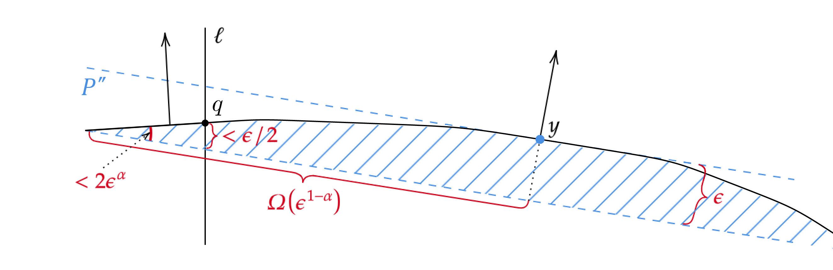
Consider the plane $\gamma$ spanned by $\mathrm{\ell }$ and a point $y$ at which the upper boundary plane of $P_i^{\prime \prime }$ touches $B(K_{i-1})$. Set

See Figure 3. If $Q$ intersects $\mathrm{\ell }$, then let $q$ denote the upper intersection point of the boundary of $Q$ with $\mathrm{\ell }$. If $Q$ does not intersect $\mathrm{\ell }$, then let $q$ be the point of $Q$ closest to $\mathrm{\ell }$, i.e., the endpoint of the “base” of $Q$ closer to $\mathrm{\ell }$.

In both cases, the angle between the normal vector to the boundary of $\gamma \cap B(K_{i-1})$ at $q$ and the normal at $y$ is at most $2{ϵ}^{\alpha }$, because the normal vectors of all planks $P_1,\mathrm{\dots },P_m$ are within an angle of at most ${ϵ}^{\alpha }$ from the vertical direction $n$ (which is the same as the direction of $\mathrm{\ell }$). The height of $Q$ at $y$, i.e., the intersection of $Q$ with a vertical line through $y$, is at least $ϵ$, while its height at $q$ is at most $ϵ/2$, by the assumption of Case B. This implies that the base of $Q$ has length $\mathrm{\Omega }({ϵ}^{1-\alpha })$.

Stepping out of the plane $\gamma$, we find that the intersection of $P_i^{\prime \prime }$ with $B(K_{i-1})$ cuts out a whole 2-dimensional face. This face contains a disk of radius $\mathrm{\Omega }({ϵ}^{1/2})$, since, as before, $B(K_{i-1})$ contains a unit ball that is tangent to the boundary of $B(K_{i-1})$ at the point $y$. Combining the last two facts, we obtain that the area of the face cut out by $P_i^{\prime \prime }$ is $\mathrm{\Omega }({ϵ}^{1-\alpha })\cdot \mathrm{\Omega }({ϵ}^{1/2})=\mathrm{\Omega }({ϵ}^{3/2-\alpha })$. Thus, $B(K_{i-1})\cap P_i^{\prime \prime }$ contains a cone with base of area $\mathrm{\Omega }({ϵ}^{3/2-\alpha })$ and height $ϵ$. This implies that

Therefore, in Case B, we have that

To complete the proof of the upper bound in Theorem 4, we iterate the above procedure. Let $k={ϵ}^{-\beta }$. As before, by averaging over directions, for any collection of $M$ planks there exists a direction $n$ such that at least $c{ϵ}^{2\alpha }M$ of them have normals within angle ${ϵ}^{\alpha }$ of $n$. In particular, at the first stage we find a subcollection of size $\mathrm{\Theta }({ϵ}^{2\alpha -\beta })$ and apply the argument of Cases A and B.

After removing the planks used in this stage, we repeat the same argument on the remaining family. As long as the number of remaining planks is at least $k/2$, the same averaging argument yields at each stage a subcollection of size $\mathrm{\Theta }({ϵ}^{2\alpha -\beta })$, so the bounds obtained above apply for each such subcollection.

Since each stage removes at most $O({ϵ}^{2\alpha -\beta })$ planks, after $t$ stages the total number removed is $O(t{ϵ}^{2\alpha -\beta })$. Choosing $t=\mathrm{\Omega }({ϵ}^{-2\alpha })$ sufficiently small in the constant factor, we ensure that at least $k/2$ planks remain throughout. Thus the procedure can be repeated $\mathrm{\Omega }({ϵ}^{-2\alpha })$ times.

Combining (3) and (4), each stage removes volume at least

Therefore the total removed volume of $B(B^3)$ is at least

Choose $\alpha$ such that $2+2\alpha -2\beta =5/2-\alpha -\beta$, that is, $\alpha =\frac{1}{6}+\frac{1}{3}\beta$. Then the above minimum is equal to $\mathrm{\Omega }(\min \{{ϵ}^{\frac{7}{3}-\frac{4}{3}\beta },$ ${ϵ}^{-\frac{1}{3}-\frac{2}{3}\beta }\})$. In view of (2), if this value is bigger than the volume of $B(B^3)$, then we must have covered the entire ball $B^3$, and we are done. If we put $\beta =\frac{7}{4}$, then this quantity is $\mathrm{\Omega }(1)$. This means that taking $k=C{ϵ}^{-7/4}$ with a sufficiently large $C$ is enough to cover $B^3$.

This completes the proof of the theorem. ∎

In the present note, we focused on the non-dissective covering problem in three dimensions. For $d>3$, the same lower bound remains valid: indeed, in order to cover a ball in ${ℝ}^d$, one needs to cover any of its $3$-dimensional sections. One may try to go into the proof and adapt the lower bound argument to the $d$-dimensional case. We should then take $\mathrm{\Omega }({ϵ}^{-2(d-1)/d})$ points on the sphere with pairwise distances at least $10{ϵ}^{2/d}$. The same analysis should lead to a slightly stronger lower bound ${ϵ}^{-2(d-1)/d}.$ The exponent in the bound does not grow linearly with $d$, because Lemma 5 guarantees only one “short” direction in the intersection of a plank and the remaining body.

The proof of the upper bound can also be extended to $d>3$, and the resulting bound would be $C_d{ϵ}^{-\frac{d+1}{2}+\frac{d-1}{d^2-d+2}}$, which is better than (1), albeit by an additive term in the exponent that tends to $0$ as $d$ grows. We believe that neither the lower nor the upper bound is tight.

The proof of the upper bound extends to $d>3$ with only minor changes. Let $k={ϵ}^{-\beta }$ and fix $\alpha >0$. By averaging over $S^{d-1}$, there exists a direction $n$ such that at least

planks have normals within angle ${ϵ}^{\alpha }$ of $n$, since a spherical cap of angular radius ${ϵ}^{\alpha }$ has measure $\mathrm{\Theta }({ϵ}^{(d-1)\alpha })$.

We proceed as in Section 3, distinguishing Cases A and B.

Case A. As before, if at least $m/2$ steps reduce the intersection of $\mathrm{\ell }$ with $B(K_i)$ by at least $ϵ/2$, then we remove from the unit ball a cap of height $\mathrm{\Omega }(mϵ)$. For $mϵ=o(1)$, such a cap has volume $\mathrm{\Omega }({(mϵ)}^{(d+1)/2})$. Hence
$$\text{Vol }B(K_0)-\text{Vol }B(K_m)\ge \min \{\mathrm{\Omega }\left({(mϵ)}^{(d+1)/2}\right),\mathrm{\Omega }(1)\}=\min \{\mathrm{\Omega }\left({ϵ}^{\frac{d+1}{2}(1+(d-1)\alpha -\beta )}\right),\mathrm{\Omega }(1)\}.$$

Case B. The planar argument in $\gamma$ is unchanged and yields a segment of length $\mathrm{\Omega }({ϵ}^{1-\alpha })$. Passing to $d$ dimensions, the boundary of $B(K_{i-1})$ contains a $(d-2)$-dimensional ball of radius $\mathrm{\Omega }({ϵ}^{1/2})$, hence the exposed $(d-1)$-dimensional face has measure $\mathrm{\Omega }({ϵ}^{d/2-\alpha })$. Therefore

and summing over the $m$ steps gives

Repeating the argument $\mathrm{\Omega }({ϵ}^{-(d-1)\alpha })$ times, we obtain a total contribution of order

Balancing the first and third exponents gives

Substituting and setting the exponent to zero yields

Thus

This improves (1), although only by an additive term in the exponent that tends to $0$ as $d\to \mathrm{\infty }$. We believe that neither the lower nor the upper bound is tight.

Our upper bound argument in Section 3 can be easily turned into a polynomial-time algorithm for constructing a cover. Take $k=C{ϵ}^{-7/4}$ planks of width $ϵ$. We first iteratively construct an ordering of the planks which will turn out to guarantee that we end up with a cover. For this, first we (approximately) compute the angle between any two normal vectors and construct a graph $G$ whose vertices are the selected $k$ planks. Two vertices are joined by an edge if the angle between the normal vectors of the corresponding planks is smaller than ${ϵ}^{\alpha }={ϵ}^{3/4}$. Then, at each step, we

1. (a)

   find a vertex $v$ whose degree is at least the average degree in $G$;

2. (b)

   include $v$ and its neighbors in the ordering (the order within this set is arbitrary);

3. (c)

   modify $G$ by deleting $v$ and its neighbors from $G$.

In the proof of the upper bound, at each step, we actually work with a chunk of vectors that were included in the ordering in one step.

Finally, we construct the covering, i.e., we find suitable translates of the planks that cover the ball, as follows. For the $i$-th plank in the ordering, we need to find the maximum (or an approximate maximum) of a linear function over the convex set $K$ that remains from the original ball after removing all points covered by the first $i-1$ planks. Then we modify the set $K$ by including an extra linear inequality in its definition, and repeat the whole procedure, if necessary.

References

- [1] Gábor Ambrus, Julian Huddell, Maggie Lai, Matthew Quirk, and Elias Williams. Covering spiky annuli by planks. Discrete & Computational Geometry, 2025. doi:10.1007/s00454-025-00799-2.
- [2] Keith Ball. The plank problem for symmetric bodies. Inventiones Mathematicae, 104(3):535–543, 1991. doi:10.1007/BF01245089.
- [3] Thøger Bang. On covering by parallel strips. Matematisk Tidsskrift B, pages 49–53, 1950.
- [4] Thøger Bang. A solution of the plank problem. Proceedings of the American Mathematical Society, 2(6):990–993, 1951. doi:10.1090/S0002-9939-1951-0046672-4.
- [5] András Bezdek. Covering an annulus by strips. Discrete & Computational Geometry, 30(2):177–180, 2003. doi:10.1007/s00454-003-0002-y.
- [6] Peter Brass, William O. J. Moser, and János Pach. Research Problems in Discrete Geometry. Springer, New York, 2005. doi:10.1007/0-387-29929-7.
- [7] László Fejes Tóth. Research problems: Exploring a planet. American Mathematical Monthly, 80(9):1043–1044, 1973.
- [8] Werner Fenchel. On Th. Bang’s solution of the plank problem. Matematisk Tidsskrift B, pages 49–51, 1951.
- [9] Helmut Groemer. On coverings of convex sets by translates of slabs. Proceedings of the American Mathematical Society, 82(2):261–266, 1981. doi:10.1090/S0002-9939-1981-0609663-7.
- [10] Helmut Groemer. Covering and packing properties of bounded sequences of convex sets. Mathematika, 29(1):18–31, 1982. doi:10.1112/S0025579300012122.
- [11] Helmut Groemer. Some remarks on translative coverings of convex domains by strips. Canadian Mathematical Bulletin, 27(2):233–237, 1984. doi:10.4153/CMB-1984-033-9.
- [12] Zilin Jiang and Alexandr Polyanskii. Proof of László Fejes Tóth’s zone conjecture. Geometric and Functional Analysis, 27(6):1367–1377, 2017. doi:10.1007/s00039-017-0427-6.
- [13] Andrey Kupavskii and János Pach. Simultaneous approximation of polynomials. In Discrete and Computational Geometry and Graphs (JCDCGG 2015), volume 9943 of Lecture Notes in Computer Science, pages 193–203, Cham, 2016. Springer. doi:10.1007/978-3-319-48532-4_17.
- [14] Andrey Kupavskii and János Pach. From Tarski’s plank problem to simultaneous approximation. American Mathematical Monthly, 124(6):494–505, 2017. doi:10.4169/amer.math.monthly.124.6.494.
- [15] Endre Makai, Jr. and János Pach. Controlling function classes and covering Euclidean space. Studia Scientiarum Mathematicarum Hungarica, 18(2–4):435–459, 1983.
- [16] Oscar Ortega-Moreno. An optimal plank theorem. Proceedings of the American Mathematical Society, 149(3):1225–1237, 2021. doi:10.1090/proc/15228.
- [17] Alfred Tarski. Uwagi o stopniu równoważności wielokątów. Parametr, 2:310–314, 1932.
- [18] William Verreault. Plank theorems and their applications: A survey. Bulletin of the London Mathematical Society, 2025. doi:10.1112/blms.70230.
- [19] Stuart White and Laura Wisewell. Covering polygonal annuli by strips. Discrete & Computational Geometry, 37(4):577–585, 2007. doi:10.1007/s00454-007-1305-z.