Computing Hausdorff Distances Under Translations: The Interplay of Dimensionality, Symmetry and Discreteness

Abstract
To measure the similarity of the shape of point sets, rather than their mere closeness in space, various notions of a Hausdorff distance under translation have been investigated. Specifically, let and denote point sets of and points, respectively, in . We consider the task of computing the minimum distance over an admissible set of translations , where denotes the Hausdorff distance under the -norm. As variants, we distinguish between continuous () or discrete ( is a given finite set of translations) as well as directed or undirected (choosing the directed or undirected Hausdorff distance for ).
We seek to apply the paradigm of fine-grained complexity to understand the complexity of these variants, and in particular: How is the running time influenced by the dimension , the relationship between and , and the specific choice of variant? As our main results, we obtain:
-
The asymmetric definition of the most studied variant, the continuous directed Hausdorff distance, results in an intrinsically asymmetric time complexity: While (Chan, SoCG’23) established a symmetric upper bound for all and proved it to be conditionally optimal for combinatorial algorithms whenever , we show that this lower bound does not hold for the case , by providing a combinatorial, almost-linear-time algorithm for and . We further prove general, i.e., non-combinatorial, conditional lower bounds for , in particular: (1) for small and (2) for and small .
-
We observe that the directed and undirected case is closely related, in particular, all our lower bounds for hold for both the directed and undirected variant. A remarkable exception is the case of for which we provide a conditional separation. Specifically, in contrast to the undirected variants being solvable in near-linear time (Rote, IPL’91), we show that the directed variants are at least as hard as the additive problem MaxConv LowerBound introduced in (Cygan, Mucha, Wegrzycki and Wlodarczyk, TALG’19).
-
We show that the discrete variants reduce to a variant of 3SUM for . This gives a barrier in proving a tight lower bound of these variants under the Orthogonal Vectors Hypothesis (OVH); in contrast, the continuous variants admit a tight conditional lower bound under OVH in (Bringmann, Nusser, JoCG’21).
These results reveal an intricate interplay of dimensionality, symmetry and discreteness in determining the fine-grained complexity of computing Hausdorff distances under translation.
Keywords and phrases:
Hausdorff Distance, Fine-Grained Complexity, Computational Geometry, Translation-Invariant Similarity MeasuresFunding:
Geri Gokaj: Partially supported by the Deutsche Forschungsgemeinschaft (DFG, German Research Foundation) – 462679611.Copyright and License:
![[Uncaptioned image]](x1.png) © Sebastian Angrick, Kevin Buchin, Geri Gokaj, and Marvin Künnemann; licensed under Creative Commons License CC-BY 4.0
© Sebastian Angrick, Kevin Buchin, Geri Gokaj, and Marvin Künnemann; licensed under Creative Commons License CC-BY 4.0
2012 ACM Subject Classification:
Theory of computation Problems, reductions and completeness ; Theory of computation Computational geometryAcknowledgements:
The authors would like to thank Jean Cardinal, Anita Dürr, Nick Fischer, Virginia Vassilevska Williams, and Karol Węgrzycki for stimulating discussions and contributions during the early stages of this work, as well as the Lorentz center and the organizers of its workshop on Fine-Grained & Parameterized Computational Geometry for facilitating these discussions.Editors:
Hee-Kap Ahn, Michael Hoffmann, and Amir NayyeriSeries and Publisher:
 Leibniz International Proceedings in Informatics, Schloss Dagstuhl – Leibniz-Zentrum für Informatik
1 Introduction
Consider the classic Hausdorff distance of given point sets and , which comes in two flavors: the directed Hausdorff distance , as well as the undirected Hausdorff distance . Here and throughout the paper, we fix our metric space to be . The two variants are sometimes also referred to as one-sided/bidirectional or one-way/two-way. Furthermore, yields a metric, in contrast to . For any constant and point sets and of and points in , we can compute these distance in near-linear time111Throughout the paper, we use , to hide polylogarithmic terms in and . Since we assume to be constant, this includes factors of the form . using -nearest neighbor search, e.g., in a range tree [18].
A computationally more challenging task is to compute the Hausdorff distance under some transformation, i.e., to minimize the Hausdorff distance of and among all sets obtained from using a set of admissible transformations. Such notions are well-studied from the perspective of shape matching or geometric pattern matching, see, e.g. [3, 4], where and model geometric objects and we are interested in comparing their general shapes rather than their mere closeness in space. In this paper, we focus on arguably one of the most basic settings, i.e., computing Hausdorff distances under translation. Specifically, when denotes a set of admissible translations, the Hausdorff distance under translation is defined as where denotes either the directed or undirected Hausdorff distance, i.e., .
The most popular setting is , which yields the natural translation-invariant version of the Hausdorff distance; we refer to this as the (continuous) Hausdorff distance under translation (HuT). This measure has received significant interest from the computational geometry community both for and other norms [20, 16, 17, 21, 11, 10, 5, 7, 9], yet only for tight upper and conditional lower bounds are known (see below for details).
Another natural version is to let be a finite set given as part of the input. We refer to this as the discrete Hausdorff distance under translation (DiscHuT). This version occurs naturally in the context of approximating the (continuous) Hausdorff distance under translation. More precisely, computing an -approximation for the continuous version can be achieved by choosing many translations such that . Since we can compute the discrete Hausdorff distance under translation in time , this yields baseline -approximation algorithms for the continuous Hausdorff distance under translation with running time ; see also [15, 22]. Consequently, obtaining faster algorithms for the discrete Hausdorff distance under translation transfers to faster approximation algorithms for the continuous version. Furthermore, the discrete version recently received interest from the perspective of a structural fine-grained complexity theory: the directed discrete Hausdorff distance under translation is part of a problem pair that is fine-grained complete for the class , a class of polynomial-time problems formed from first-order properties on finite additive structures [14] (further discussion can be found in the full version).
Previous works on Hausdorff distances under translation mostly focus –with notable exceptions such as [7, 9]– on a single particular variant, often considering particular dimensions and the balanced case, in which all inputs sets (i.e., , , and in the discrete case also ) have roughly equal size . In this work, we aim to give a more comprehensive analysis, which reveals an intricate interplay between the dimensionality, symmetry (directed/undirected and the relationship between and ), and discreteness.
1.1 Our Results
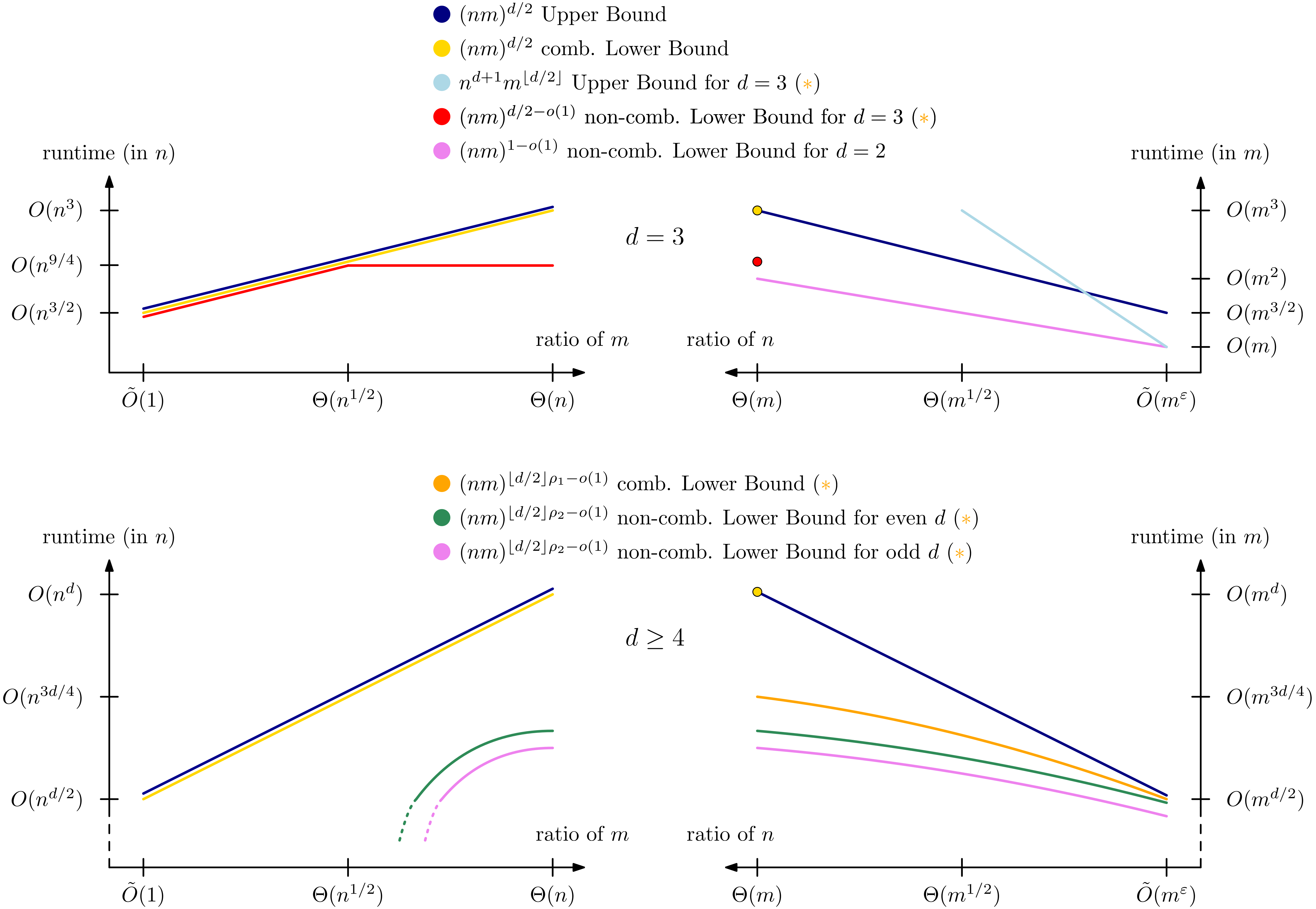
Our first question concerns the fine-grained complexity of the algorithmically most studied variant, the (continuous) directed Hausdorff distance under translation. The currently best upper bounds are for [11], for [10]222While [10] only considers the case , their analysis also holds for distinct . A short explanation of their approach can also be found in the full version., and for general [9]. This suggests the following question:
Question 1: Is the time complexity of directed Hausdorff -distance under Translation?
A conditional lower bound of Bringmann and Nusser [7] (based on the Orthogonal Vectors Hypothesis) answers this question positively for . Subsequently, Chan [9] gave evidence of optimality even for , by proving a conditional lower bound of for combinatorial algorithms333Here, combinatorial algorithms refers to algorithms that avoid the use of algebraic techniques underlying fast matrix multiplication algorithms beating running time. in the case that . However, proving such a conditional lower bound against general algorithms for (or better conditional lower bounds than for the case ) remained open until this work. Furthermore, for , no algorithms are known, raising the question whether any superlinear lower bound can be proven for .
As our first main contribution, we give a perhaps surprising negative answer to Question 1: For and , there exists an almost-linear time algorithm, showing that in an unbalanced setting, the upper bound of can indeed be beaten (Section 3.4). Interestingly, this stands in contrast to the case of moderately small : For and any we prove a tight conditional lower bound of , by combining the proof techniques of Chan’s combinatorial -clique lower bound [9] and the tight 3-uniform hyperclique lower bound for Klee’s measure problem in 3D [19] (Section 3.2). This reveals that the time complexity of the directed Hausdorff distance under translation is inherently asymmetric in and and breaks with tradition for algorithmic results on the Hausdorff distance under translation.
We investigate the case of small further and observe that our algorithmic approach could plausibly generalize to an algorithm (we elaborate on the missing ingredient in Section 3.4) – such an algorithm would beat the baseline algorithm for all odd and small values of . We also show that such an algorithm would indeed be conditionally tight: we also prove a corresponding lower bound of for all , assuming the 3-uniform hyperclique hypothesis (Section 3.1).
Our conditional lower bounds can be adapted to the case of , but no longer match the upper bound. In fact, we obtain a conditional lower bound of for which still leaves a gap of to the upper bound of . It remains an open problem to settle the full time complexity for any relationship between and . An intriguing possibility consistent with our results is the existence of an -time algorithm.
We turn to our second main question.
Question 2: How does the choice of dimension, directed vs. undirected and discrete vs. continuous affect the time complexity?
We observe that the time complexity of computing Hausdorff distances under translation exhibits an intricate interplay between the different aspects of the problem, illustrated in Table 1 and Figure 1.
On directed vs. undirected
A folklore reduction from computing the undirected Hausdorff distance to computing the directed Hausdorff distance under translation (˜2.3) shows that the undirected case is never harder than the (balanced) directed case. Could there exist a reduction in the other direction?
We show that in full generality, such a reduction appears unlikely: While for all , we can transfer our conditional lower bounds for the directed case to analogous bounds in the undirected case (analogous to the OVH-based lower bound for [7], which also transfers to the undirected case) (Section 3.5), we obtain a conditional separation for . Notably, Rote [20] obtains a -time algorithm for computing the undirected Hausdorff distance under translation in . For the directed setting, we give a fine-grained reduction from the quadratic-time -Necklace Alignment problem [6], which in turn is at least as hard as the MaxConv LowerBound problem studied in [12]. We remark that we are not aware of any conditional lower bound for MaxConv LowerBound under an established hypothesis from fine-grained complexity theory; however, the question of subquadratic equivalence between this problem and the well-studied -convolution problem was raised as an open problem in 2017 [12]. We believe that our reduction to the (discrete or continuous) directed Hausdorff distance adds further reason to study the apparent quadratic-time complexity of MaxConv LowerBound, in hopes to either refute or justify this hardness barrier.
Circumventing the separation in , we give a general reduction from the undirected setting to the directed setting that blows up the dimension (Section 3.5). This allows us to transfer the lower bounds from the directed case for to the undirected case in . In particular, we conclude that if MaxConv LowerBound truly requires quadratic-time, the undirected setting is near-linear time solvable if and only if .
On discrete vs. continuous
The tight lower bound based on OVH [7] convincingly settles the fine-grained complexity of the continuous setting in . In contrast, the only justification of hardness of the discrete setting is given by our reductions from MaxConv LowerBound and -Necklace Alignment (see above and the full version). Is there any reason why a tight lower bound based on OVH does not exist for the discrete setting?
We find evidence for the non-existence of such a reduction by showing a fine-grained reduction from (directed or undirected) discrete Hausdorff distance under translation in to the All-Ints 3SUM problem (in the full version). In particular, this implies a tight fine-grained reduction from the balanced setting to 3SUM. Thus, establishing quadratic-time OVH-hardness of the balanced, discrete setting implies a tight reduction from OV to 3SUM, which is a central open problem in fine-grained complexity theory, and suffers from barriers based on the Nondeterministic Strong Exponential Time Hypothesis, see [8].
We remark that we obtain further connections from the class of additive problem to the discrete variants. For space reasons, these results are deferred to the full version.
2 Preliminaries
A brief definition of relevant problems as well as the used hardness hypotheses can be found in the full version. We there also give a brief overview of known algorithms for the continuous and discrete variant.
We recall the Hausdorff distance as a distance measure between two point sets of sizes . The metric space used for this paper will be . The undirected (symmetric) and directed (asymmetric) variant are defined as:
We show almost all of our conditional lower bounds already for the decision variant of Hausdorff under Translation, which receives a test distance as additional input444Note that the case , i.e., finding an exact match, allows an almost-linear-time algorithm [13] and is thus uninteresting for our purposes.. Clearly, the corresponding optimization problems, finding a translation minimizing , are at least as hard. Specifically, we study:
Definition 2.1 (Hausdorff under Translation (HuT)).
Given sets of and points, respectively, and a real value . Decide whether:
Definition 2.2 (Discrete Hausdorff under Translation (DiscHuT)).
Given sets of and points, respectively, a real value as well as a set of at most translations . Decide whether:
Note that our definition of the discrete variant assumes all input entries to be polynomially bounded integers555One may also assume rational coordinates, which is equivalent by a scaling argument..
To obtain the undirected versions of the above problems, we replace by , and denote the problem by (Disc)uHuT. If not specified otherwise, we consider the directed versions. We call the case in which all input sets have roughly equal size, i.e., and additionally for the discrete case , the balanced parameter setting, otherwise we say the parameters are lopsided.
Lastly, we give a folklore reduction from undirected to directed Hausdorff under Translation that works for both the continuous and discrete variant. By setting for a sufficiently large , we see that .
Observation 2.3.
The undirected (Discrete) Hausdorff under Translation problem with input sizes reduces to the directed version with input sizes .
While this reduction introduces additional points to the input, we discuss in the full version that an input size maintaining reduction to a single instance of directed HuT is unlikely.
As our model of computation, we use the Real RAM for continuous HuT, while for the discrete HuT variant with point sets in we assume a Word RAM machine model with word size .
2.1 Translation Problems
For clarity of presentation, it is often useful to view the Hausdorff under Translation decision problem as a translation problem involving certain shapes.
Definition 2.4 (Translation Problem).
Given a set of points and shapes in . Compute a translation such that
For an instance of HuT with point sets and , if we construct hypercubes with side length and centers , the region is exactly the region of feasible translations, i.e., we have [1]. We call this case, where all shapes are hypercubes of the same size, the Translation Problem with Hypercubes (TPwC). In case all shapes of are axis-aligned boxes (of arbitrary size), we call it the Translation Problem with Boxes (TPwB). While the TPwC problem is equivalent to HuT, there is no reduction to HuT known within the same ambient space from the Translation Problem with Boxes or even from the translation problem with hypercubes of different sizes. We further use a third variant.
Definition 2.5 (Translation Problem with Orthants (TPwO)).
Given a target box with a maximum side length . Given a set of Translation Problem with Hypercube instances, each on a point set and hypercubes with side length , such that , . Compute a translation such that and
We call the shapes of the TPwO instance, i.e., the shapes of its sub-instances, orthants as within the target box all hypercubes are indistinguishable from orthants. An important property of this problem, which we will use later, is that we may fix the side-length of all orthants to a value . Similar to [9, Lemma 3], the TPwO problem reduces to the TPwC and thus has a reduction to HuT, its proof is deferred to the full version. A converse reduction, from HuT to TPwO, is generally not known.
Lemma 2.6.
The Translation Problem with Orthants on points and orthants reduces in linear time to the Translation Problem with Hypercubes on points and hypercubes.
3 Technical Overview for Selected Results
In this section, we discuss the main ideas of our lower bounds and algorithm. We present the general structure of the proofs and give sketches on the most important technical details. For space reasons, we defer further details as well as a complete discussion of our results and further extensions to the full version.
3.1 (Non-)Combinatorial Lower Bounds for Arbitrary
For our lower bounds in higher dimensions (), we give a reduction in three steps from the -hyperclique problem to HuT, see the full version for a formal definition and its hardness hypothesis.
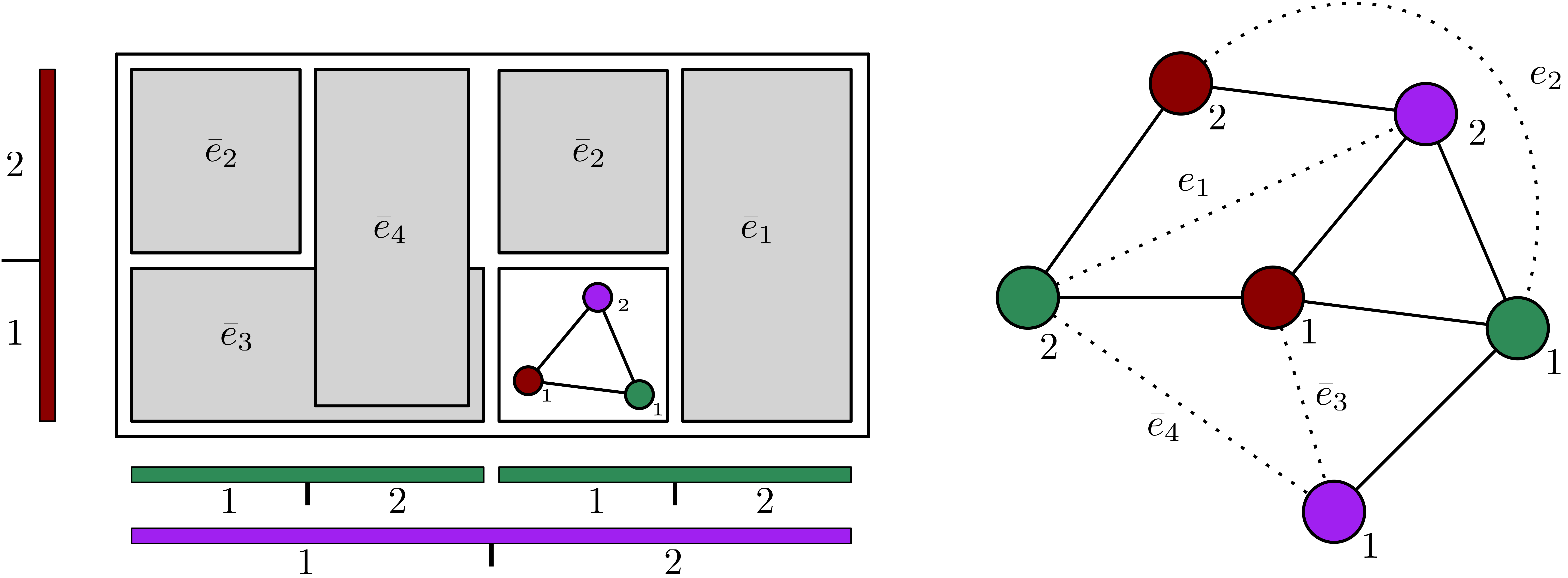
In the first step, we encode any -tuple of vertices of a hypergraph as cells inside a -dimensional hypercube, see Figure 2. The used encoding was introduced by Chan [9]. For any non-edge , the feasible region of are the cells inside the hypercube for which the corresponding -tuple does not include . In contrast, the cells for which the corresponding -tuple includes all vertices of are called the forbidden region. For each non-edge, we construct a covering of its feasible region with axis-aligned boxes666As we only consider axis-aligned boxes in this paper, we may only call these boxes., see Lemma 3.5 for the exact covering. As a -clique is a -tuple which does not contain any non-edge, a cell that lies within the feasible regions of all non-edges encodes a -clique. In Lemma 3.6 we reduce finding a cell inside all feasible regions to the intermediate Translated Box-Shape Problem (Definition 3.2) with our desired values of .
In the second step, the resulting Translated Shape Problem is reduced to the Translation Problem with Boxes, see Lemma 3.3.
Lastly, in our third step we reduce the Translation Problem with Boxes in -D to the Translation Problem with Orthants in dimensions with points and orthants, see Lemma 3.1. As given in Lemma 2.6, the Translation Problem with Orthants has a linear time reduction to directed Hausdorff under Translation, which yields our lower bound.
We go through the steps in backwards order, starting with the last, third step.
Step 3: From Boxes to Orthants
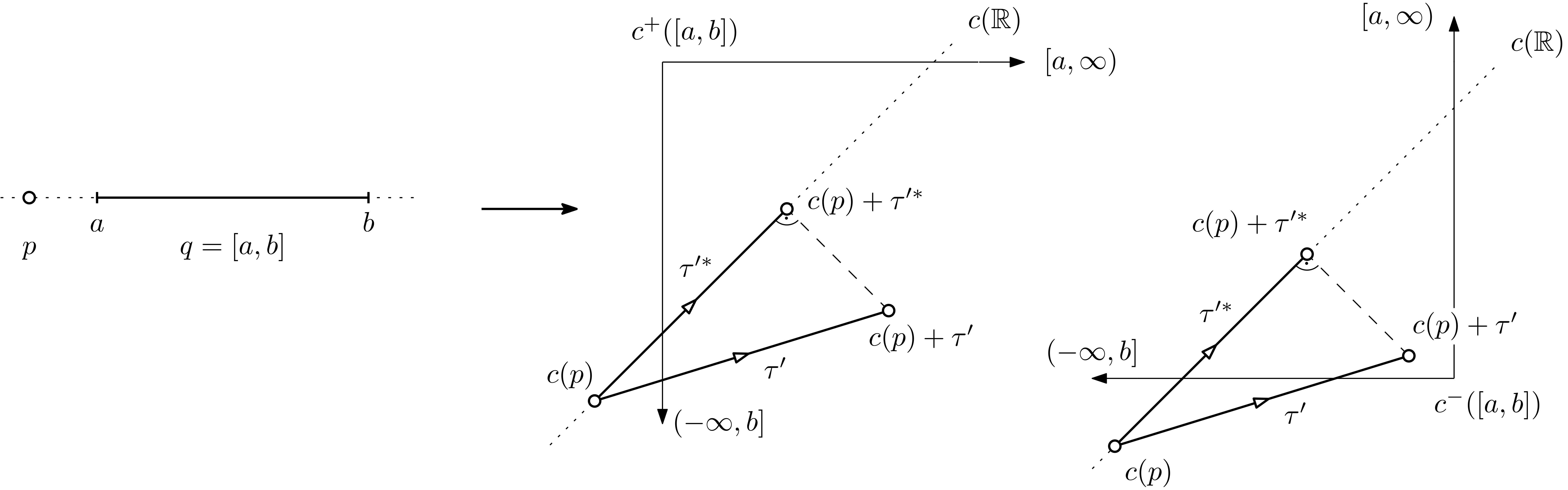
We reduce the Translation Problem with Boxes to the Translation Problem with Orthants. We implement the natural idea to cover boxes of arbitrary aspect ratios by orthants (large hypercubes), at the cost of doubling the underlying dimension. As this basic idea allows additional, unintended solutions, we need a technical translation gadget that ensures soundness. Figure 3 gives a visual intuition of the proof in -D.
Lemma 3.1.
The Translation Problem with Boxes in -D with input parameters reduces in linear time to the Translation Problem with Orthants in -D with input parameters .
Proof Sketch.
We define the coordinate-wise transformations
For points in , we define the transformation as the coordinate-wise application of . For our analysis, we further apply to sets or intervals in which case we apply element-wise. For boxes in , we define the transformations as all possible combinations of the coordinate-wise application of . Note that the images of are orthants.
Given an instance of the Translation Problem with Boxes with being the point set and being the set of boxes. We construct the sub-instances of the resulting Translation Problem with Orthants instance, the target box is simply the bounding box of . We claim that
For the proof, we see that a feasible translation for the right side for any is a feasible translation for the left side, so we prove that a feasible translation can be transformed to a feasible translation . Choosing the such that always lies on the correct side of , where all vertices of our constructed orthants lie, enables us to move to its closest point on , giving for all . The full proof details can be found in the full version.
Step 2: The intermediate Translated Box-Shape Problem
We introduce an intermediate problem, the Translated Box-Shape Problem, similar to the one of [9, Problem 4] using hypercubes. In contrast to the Translation Problem with Boxes, it allows composing boxes into shapes for which translated copies can be instantiated with a single translation object. Thus, a set of boxes, structured appropriately, can be described by a shape of boxes and translation objects.
Definition 3.2.
(Translated (Box-)Shape Problem). Let be a set of shapes in , composed of a union of boxes. Let be the total number of boxes over all shapes of . Given a set of objects where each object is the translate of some shape in , decide whether .
We further give a reduction from the Translated Shape Problem to the Translation Problem with Boxes, analog to [9, Lemma 3]. Its proof again is deferred to the full version.
Lemma 3.3.
The Translated (Box-)Shape Problem with translation objects and a total of boxes reduces to the Translation Problem with Boxes with and .
Lastly, we give a simple observation allowing, by repeated application, to compose arbitrary many individual Translated (Box-)Shape Problems without additional overhead.
Observation 3.4.
Given two instances of the Translated Shape Problem with inputs and of size and in a shared universe. Deciding whether reduces to a single instance of the Translated Shape Problem with , of size and .
Step 1: From -Hyperclique to the Translated Box-Shape Problem
In the remaining step, along the basic idea presented in the beginning of Section 3.1, we encode the -hyperclique problem to a -dimensional hypercube and reduce finding a cell that lies in the feasible regions of all non-edges to the Translated (Box-)Shape Problem with the desired distribution of parameters . As our approach will also provide novel combinatorial lower bounds, we more generally consider a -uniform hypergraph with .
We first give the encoding of the hypergraph to a -dimensional hypercube and show that the feasible regions of the non-edges can be covered efficiently. The same encoding for a graph can exemplarily be seen in Figure 2, note that for illustrative reasons we there have not covered the feasible but the forbidden regions.
Lemma 3.5.
Let and be constant and let be constant with . Given a -uniform hypergraph with , where is partitioned into color classes . There is an encoding of to a -dimensional hypercube so that for each the feasible region of can be covered by boxes, which can be computed in time.
Proof Sketch.
By scaling, we assume that the -dimensional hypercube has a side-length of . Given the numbers , we use the canonical function
to address an integer point in the range We denote each unit hypercube as a cell, its relative origin can be addressed by where .
The encoding of to the hypercube is the same as used in [9]. We evenly assign the color-classes to the dimensions, i.e., the color classes are assigned to the first dimension, the classes to the second dimension, etc. A -tuple is bijectively assigned to the cell
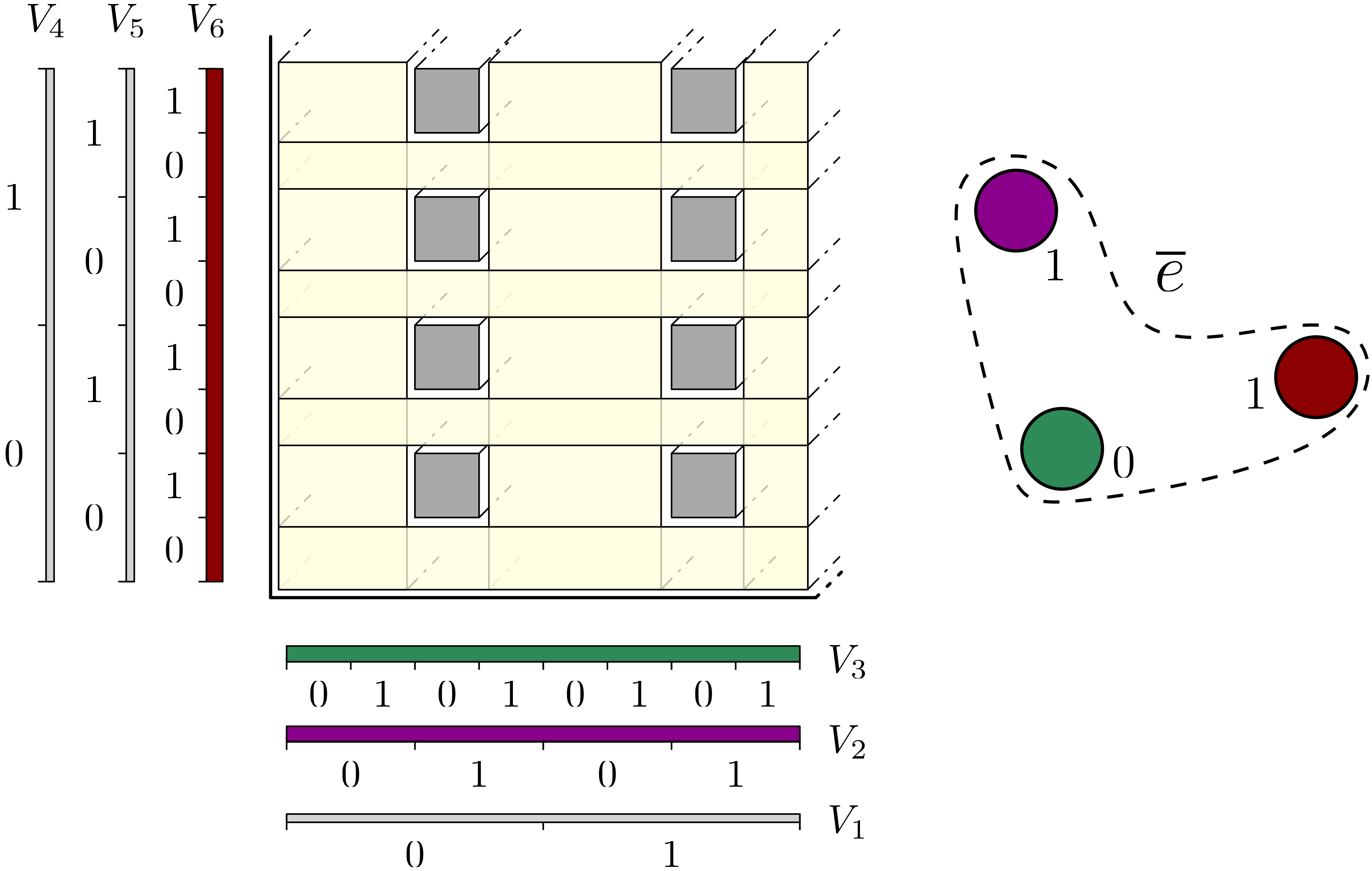
For any non-edge , we cover the feasible region of using at most boxes , as can be seen in Figure 4. A full proof can be found at in the full version.
Using Lemma 3.5, we can already turn a -(hyper-)clique instance into a Translated (Box-)Shape instance with as we can treat each feasible region of the non-edges as an independent shape with boxes each. ˜3.4 allows to compose the resulting independent instances.
To extend the reduction to arbitrary parameter choices of , independently for each non-edge we decompose the hypercube into smaller identical parts such that in each part the feasible region of a non-edge can be covered by boxes as shown in Lemma 3.5. This allows a reduction to the Translated Shape Problem with boxes and translation objects.

Right: The boxes used to cover the feasible region of the green sub-regions, in yellow, as well as the boxes covering the complement of the green sub-region, marked in pink.
Lemma 3.6.
Let , be constant, and be constants with . Given a -regular hypergraph and its encoding to a -dimensional hypercube as constructed in Lemma 3.5. We reduce the problem of finding a -(hyper-)clique in in time to an instance of the Translated (Box-)Shape Problem with translates of common shapes consisting of boxes.
Proof Sketch.
By ˜3.4, it suffices to consider the feasible regions of a single non-edge and reduce finding a cell that lies in its feasible regions to a Translated (Box-)Shape instance with translates of a single shape with boxes.
We consider the encoding of the hypergraph to the -dimensional hypercube as given in Lemma 3.5. As is a -tuple, its included vertices are only encoded in up to dimensions, it thus suffices to consider the hypercube projected to these dimensions.
We construct many sub-regions that decompose the -dimensional hypercube: We decompose each single dimension into many (not necessarily continuous) slices that are identical under translation, i.e., when translated so that two slices have the same relative origin, the feasible and forbidden regions of within these slices match. These one-dimensional slices can be combined independently in all dimensions, yielding the desired decomposition of the full -dimensional hypercube into identical sub-regions.
The feasible region of in each sub-region can be covered by boxes. As the sub-regions are identical, we can construct a Translated (Box-)Shape instance with translation objects and a single shape with boxes. A full proof can be found in the full version.
Resulting Lower Bounds
Combining our results from Lemmas 3.6, 3.3, and 3.1, we get lower bounds for arbitrary distributions of . However, as the bounds deteriorate with growing values of , we only get tight lower bounds for . We consider other cases in the full theorem statement which can be found with its proof in the full version.
Theorem 3.7.
Let be constant. Under the -hyperclique hypothesis, there is no algorithm for directed HuT in -D with .
3.2 Tight Non-Combinatorial Lower Bound in -D
Chan [9] has proven a tight lower bound that applies for distributions in -D. We give a non-combinatorial version of this lower bound for .
We reduce from the -Hyperclique problem, combining Chan’s ideas with the work of Künnemann [19] using prefix covering designs. As done in Section 3.1, we encode a -tuple of vertices inside a -dimensional hypercube. However, we use a redundant encoding based on the prefix covering designs, that is, each color class is encoded more than once to our hypercube. The full proof is presented in the full version.
Corollary 3.8.
Let . For any , there is no (non-combinatorial) algorithm for directed Hausdorff under Translation in -D with under the -hyperclique hypothesis.
3.3 Connections to Additive Problems
We draw several connections between the Hausdorff distance under Translation and several additive problems. Below we highlight a conditional lower bound in 1D and conditional upper bound in 3D. Omitted proofs and additional results are given in the full version.
We first show that even for one-dimensional instances, directed HuT inherits hardness from quadratic-time barriers from problems such as MaxConv LowerBound.
Definition 3.9 (MaxConv LowerBound, MaxConvLB).
Given integer arrays of length777Other common definitions use for an array of size . For convenience, we stick to this definition. . Determine whether holds for all .
In an investigation of hardness results from -convolution, Cygan, Mucha, Wegrzycki and Wlodarczyk [12] studied the closely related MaxConv LowerBound problem and gave a subquadratic reduction to -Necklace Alignment (in turn, -Necklace Alignment admits a subquadratic reduction to -Convolution [6]). Cygan et al. raised the natural question whether MaxConv LowerBound is subquadratic equivalent to -convolution; to the best of our knowledge, neither a positive or negative resolution is known.
For the (continuous) directed HuT we get hardness by a reduction from the Linear Alignment problem, shown in the full version. Further, using a reduction from -Necklace Alignment to Linear Alignment, we get a reduction from MaxConv LowerBound to directed HuT. Interestingly, we obtain such a lower bound even for discrete directed HuT by directly reducing from MaxConv LowerBound. These reductions illuminate why no subquadratic algorithms are known for directed variants, despite near-linear algorithms for their undirected counterparts [20].
Theorem 3.10.
If 1-dimensional discrete HuT can be solved in time , then the MaxConv LowerBound problem can be solved in time
Proof sketch.
Given arrays of positive values as inputs from MaxConv LowerBound. We construct as arrays for DiscHuT. By abuse of notation, we allow to be indexed negatively. We define , , , , where is a large number with .
Now, if is a NO-instance to MaxConv LowerBound, then there is a such that for all we have . From this we can derive that , where , , and denote the points in , , and , respectively, corresponding to , and . Thus, we have a YES-instance to DiscHuT. Analogously, a YES-instance to MaxConv results in a NO-instance to DiscHuT. See the full version for the full proof.
We give an upper bound to discrete HuT, which stems from a reduction from 3-dimensional Discrete HuT to 3-SUM. On a very high level, the basic idea consists of a complement trick, which enables a quantifier switch in the discrete HuT problem.
Corollary 3.11.
Let . If -SUM can be solved in time , then we can solve -dimensional balanced Discrete HuT in time
3.4 A Faster Algorithm for
For , Theorem 3.7 gives a lower bound, which for even matches the best known algorithm running in time [9], while for odd it seems to have some slack. Intuitively, one might expect that the known combinatorial lower bound for [9] also transfers to the case of . Surprisingly, in -D the lower bound of [7] is tight for as we give an algorithm.
The algorithm uses a structural insight from [10, Theorem 7], which we turn algorithmic. The full description and proof can be found in the full version. Our algorithm relies on an algorithm recently introduced by Agarwal and Steiger [2], which in -D computes the vertices of the union of unit cubes in an output-sensitive runtime of . Assuming an algorithm that computes the vertices of the union of unit hypercubes in -D in time , our algorithm directly generalizes to higher dimensions with a runtime of .
Theorem 3.12.
Directed Hausdorff under Translation in -D can be solved in time .
Its existence forbids lower bounds for arbitrary distributions of for , and we give compelling intuition for a similar result in odd .
Corollary 3.13.
Let , and set . For , directed Hausdorff under Translation in -D can be solved in time .
This result points to a discrepancy in complexity, at least for but potentially also for all odd . While we have a algorithm for , there is a tight (combinatorial) lower bound for [9]. It remains unknown where the cutoff point is located, i.e., for which values of do we start to get faster than algorithms?
3.5 Transferring Lower Bounds to the Undirected Setting
As of now, all here presented lower bounds only apply to the directed Hausdorff under Translation setting. Chan [9] already raised the question if these bounds transfer to the undirected setting, however there are no such lower bounds known so far for . Only for , lower bounds for the undirected setting are known [7], which match the bounds for the directed variant. For , we have an optimal algorithm [20].
We partially resolve this question by providing a reduction from the Translation Problem with Orthants to undirected Hausdorff under Translation, maintaining all instance parameters.
Theorem 3.14.
If we can decide the undirected Hausdorff under Translation problem in -D with point sets of size in time , we can decide the Translation Problem with Orthants in -D with points and orthants in time .
Proof Sketch.
We only give intuition on the reduction to a uHuT instance from a single TPwC sub-instance of our TPwO input. The full proof is given in the full version.
For an individual TPwC instance, given the point set and the set of hypercubes of side length . Note that the target box of our TPwO instance implies that the translated point set and the set of feasible translations is restricted, we may assume that and , where is some relative origin.
We strategically place additional points in the TPwC sub-instance to allow a reduction to uHuT. These points are located on the vertices and middle points of all faces of a extended target box. As the translation and translated point set are restricted, any hypercube that intersects the target box also intersects the extended target box when translated. Thus, we can place auxiliary points such that under all translations each hypercube of our TPwC instance has an auxiliary point which lies inside . Having this property, the reduction to uHuT is imminent. All lower bounds for HuT in dimensions presented so far, as well as the combinatorial lower bound for of Chan [9], can be directly applied to undirected Hausdorff under Translation as they use the Translation Problem with Orthants as an intermediate problem. At the cost of doubling the dimension using Lemma 3.1, we generally reduce any instance of directed Hausdorff under Translation to the undirected setting.
Corollary 3.15 (Excerpt from full version).
We get the following results:
-
For arbitrary , there is no combinatorial algorithm for undirected Hausdorff under Translation in -D under the -clique hypothesis.
-
For , there is no algorithm for undirected Hausdorff under Translation in -D under the -hyperclique hypothesis.
-
If balanced (discrete) undirected Hausdorff under Translation in -D can be solved in time , then MaxConv LowerBound can be solved in time .
References
- [1] P. K. Agarwal, M. Sharir, and S. Toledo. Applications of parametric searching in geometric optimization. J. Algorithms, 17(3):292–318, 1994. doi:10.1006/jagm.1994.1038.
- [2] Pankaj K. Agarwal and Alex Steiger. An output-sensitive algorithm for computing the union of cubes and fat boxes in 3D. proc48th, 198:10:1–10:20, 2021. doi:10.4230/LIPIcs.ICALP.2021.10.
- [3] Helmut Alt and Leonidas J. Guibas. Discrete geometric shapes: Matching, interpolation, and approximation. In Jörg-Rüdiger Sack and Jorge Urrutia, editors, Handbook of Computational Geometry, pages 121–153. North Holland / Elsevier, 2000. doi:10.1016/B978-044482537-7/50004-8.
- [4] Helmut Alt, Kurt Mehlhorn, Hubert Wagener, and Emo Welzl. Congruence, similarity, and symmetries of geometric objects. Discret. Comput. Geom., 3:237–256, 1988. doi:10.1007/BF02187910.
- [5] Gill Barequet and Sariel Har-Peled. Polygon Containment and Translation in Hausdorff-Distance Between Segment Sets are 3SUM-Hard. International Journal of Computational Geometry & Applications, 2001. doi:10.1142/S0218195901000596.
- [6] David Bremner, Timothy M. Chan, Erik D. Demaine, Jeff Erickson, Ferran Hurtado, John Iacono, Stefan Langerman, Mihai Pătraşcu, and Perouz Taslakian. Necklaces, convolutions, and X+Y. Algorithmica, 69(2):294–314, 2014. doi:10.1007/S00453-012-9734-3.
- [7] Karl Bringmann and André Nusser. Translating Hausdorff is hard: fine-grained lower bounds for Hausdorff distance under translation. J. Comput. Geom., 13(2):30–50, 2021. doi:10.20382/JOCG.V13I2A3.
- [8] Marco L. Carmosino, Jiawei Gao, Russell Impagliazzo, Ivan Mihajlin, Ramamohan Paturi, and Stefan Schneider. Nondeterministic extensions of the strong exponential time hypothesis and consequences for non-reducibility. In 7th, pages 261–270, 2016. doi:10.1145/2840728.2840746.
- [9] Timothy M. Chan. Minimum Hausdorff distance of point sets under translation: Generalizing Klee’s measure problem. In proc39th, volume 258, pages 24:1–24:13. Schloss Dagstuhl – Leibniz-Zentrum für Informatik, 2023. doi:10.4230/LIPIcs.SOCG.2023.24.
- [10] L. P. Chew, D. Dor, A. Efrat, and K. Kedem. Geometric pattern matching in -dimensional space. Discrete Comput Geom, 21(2):257–274, 1999. doi:10.1007/PL00009420.
- [11] L. Paul Chew and Klara Kedem. Getting around a lower bound for the minimum Hausdorff distance. Computational Geometry, 10(3):197–202, June 1998. doi:10.1016/S0925-7721(97)00032-1.
- [12] Marek Cygan, Marcin Mucha, Karol Wegrzycki, and Michal Wlodarczyk. On problems equivalent to (min,+)-convolution. ACM Transactions on Algorithms, 15(1):14:1–14:25, 2019. doi:10.1145/3293465.
- [13] Nick Fischer. Deterministic sparse pattern matching via the Baur-Strassen theorem. In proc35th, pages 3333–3353. SIAM, 2024. doi:10.1137/1.9781611977912.119.
- [14] Geri Gokaj and Marvin Künnemann. Completeness theorems for -SUM and geometric friends: Deciding fragments of linear integer arithmetic. In proc16th, volume 325 of LIPIcs, pages 55:1–55:25, 2025. ISSN: 1868-8969. doi:10.4230/LIPIcs.ITCS.2025.55.
- [15] Michael T. Goodrich, Joseph S. B. Mitchell, and Mark W. Orletsky. Approximate geometric pattern matching under rigid motions. IEEE Trans. Pattern Anal. Mach. Intell., 21(4):371–379, 1999. doi:10.1109/34.761267.
- [16] Daniel P. Huttenlocher, Klara Kedem, and Micha Sharir. The upper envelope of Voronoi surfaces and its applications. Discrete & Computational Geometry, 9:267–291, 1993. doi:10.1007/BF02189323.
- [17] Daniel P. Huttenlocher, Gregory A. Klanderman, and William Rucklidge. Comparing images using the Hausdorff distance. IEEE Trans. Pattern Anal. Mach. Intell., 15(9):850–863, 1993. doi:10.1109/34.232073.
- [18] Sanjiv Kapoor and Michiel Smid. New techniques for exact and approximate dynamic closest-point problems. SIAM Journal on Computing, 25(4):775, 1996.
- [19] Marvin Künnemann. A tight (non-combinatorial) conditional lower bound for Klee’s measure problem in 3D. In proc63rd, pages 555–566, 2022. doi:10.1109/FOCS54457.2022.00059.
- [20] Günter Rote. Computing the minimum Hausdorff distance between two point sets on a line under translation. Information Processing Letters, 38(3):123–127, 1991. doi:10.1016/0020-0190(91)90233-8.
- [21] William Rucklidge. Lower bounds for the complexity of the graph of the hausdorff distance as a function of transformation. Discret. Comput. Geom., 16(2):135–153, 1996. doi:10.1007/BF02716804.
- [22] Carola Wenk. Shape Matching in Higher Dimensions. PhD thesis, Freie Universität Berlin, 2003. doi:10.17169/refubium-8310.