Topological Simplification Guided by Forbidden Regions

Abstract
Topological simplification is the process of reducing complexity of a function while maintaining its essential features. Its goal is to find a new filter function, which reorders cells of the input complex in a way which eliminates some persistent homological features, without affecting the rest. We present a new approach to simplification based on the concept of forbidden regions and combinatorial dynamics. It allows us to reorder and cancel critical values, whose cancellation is not possible using existing methods because they are not consecutive in the total order. Each such cancellation takes time in the worst case, where is the number of birth-death pairs and is the size of the input complex.
Keywords and phrases:
persistent homology, topological simplification, depth posetsFunding:
Jakub Leśkiewicz: The research was partially funded by the Polish National Science Center under Opus Grant No. 2019/35/B/ST1/00874 and Opus Grant 2025/57/B/ST1/00550.Copyright and License:
![[Uncaptioned image]](x1.png) © Jakub Leśkiewicz, Bartosz Furmanek, Michał Lipiński, and Dmitriy Morozov; licensed under Creative Commons License CC-BY 4.0
© Jakub Leśkiewicz, Bartosz Furmanek, Michał Lipiński, and Dmitriy Morozov; licensed under Creative Commons License CC-BY 4.0
2012 ACM Subject Classification:
Computing methodologies Algebraic algorithms ; Mathematics of computing Algebraic topologyAcknowledgements:
Jakub Leśkiewicz wants to thank his supervisor, Prof. Marian Mrozek, for scientific guidance, patience, and opportunity to delay the rest of his duties while writing this work. The author also extends thanks to his entire family, to Zuzanna Świątek, and to Mikołaj Kardyś, BEng, MSc, for providing meals during the most intensive periods of work.Editors:
Hee-Kap Ahn, Michael Hoffmann, and Amir NayyeriSeries and Publisher:
 Leibniz International Proceedings in Informatics, Schloss Dagstuhl – Leibniz-Zentrum für Informatik
1 Introduction
Simplification of real-valued functions is one of the central topics in Morse theory. In the classical (smooth) setting, one of the most notable examples of such simplifications is performed throughout the proof of the h-cobordism theorem [25, 24]. In the discrete setting, Forman’s theory [18, 17] studies the reversal of a unique combinatorial path between two critical points as a way of reducing the total number of critical points and, therefore, simplifying the Morse complex.
More recently, simplification has been studied in the context of persistent homology. The authors of [14] introduced the problem of persistence-sensitive simplification – asking to simplify all pairs with persistence below a given threshold – and gave an algorithm for 2-manifolds. Their solution was later improved to linear time [1]. Another approach, based on Forman’s combinatorial vector fields, was presented in [3]. This work drew connection to the cancellation procedure by observing that whenever the unique path connects two critical points with locally lowest difference in function values, their cancellation does not affect the remaining part of the persistence diagram [3]. These apparent pairs have also been called close pairs [9] and shallow pairs [15].
This observation further helped in optimization of (persistent) homology computation [2] and shape reconstruction [4]. The idea of pruning pairs of critical cells, following Forman’s approach, has been extensively studied in data visualization [6, 7, 10, 16, 21, 22, 27]. Recent works on topological optimization [20, 26] offer an alternative, albeit less controlled approach to simplification.
But there remains a critical gap. The works that are able to rigorously control the changes in persistent homology [14, 1, 3] are only able to simplify 0-dimensional persistent homology (as well as codimension-1, by duality). Meanwhile, the middle dimensions – e.g., 1-dimensional homology on 3-manifolds – are important in practice.
In this work, we study how relations between persistence pairs calculated by the standard lazy reduction algorithm [11, 5] can guide us in simplifying a discrete Morse function , while controlling the changes in its persistence diagram in any dimension and the overall gradient structure. These relations organize persistence pairs in a hierarchical structure called a depth poset [12]. As observed in [13, 26], these relations describe the obstacles to modifying a function without changing its persistence diagram.
Concretely, for a given persistence pair , we define forbidden regions for its death and birth cells, which describe the parts of the persistence diagram that cannot move to without changing the persistence pairing. Conversely, when the forbidden regions leave a gap – a path from to the diagonal – we can construct a homotopy that brings to the diagonal without changing the rest of the persistence pairs and the gradient structure. This allows us to identify a broader family of persistence pairs, possibly with high persistence, that can be safely and selectively removed. We summarize our main contribution in the following theorem, where denotes the set of birth-death pairs induced by a discrete Morse function , and , the set of critical cells for .
Theorem 1.
Let be a discrete Morse function on a Lefschetz complex . If is a persistence pair such that forbidden regions of its death and birth cells do not intersect, and there exists exactly one gradient path between the paired critical cells, then there exists a discrete Morse function on such that and for all .
We present a constructive proof to this theorem, which provides an algorithm explicitly tracking all changes in relations throughout the homotopy and the final path reversal. As a result, we obtain already computed relations between pairs in , which enables iterative simplification.
2 Preliminaries
Definition 2.
A Lefschetz complex is a triplet , where is a finite set of elements called cells, is a map assigning a dimension to each cell, and is the boundary coefficient such that implies , in which case we say is a facet of . Additionally, we require that for any we have . We also define the coboundary coefficient as .
Lefschetz complexes generalize simplicial, cubical, and cellular complexes while remaining concrete enough to define persistent homology. When it does not lead to confusion, we shorten the notation and refer to the set of cells, , as the Lefschetz complex. We often interpret and as a matrix, in which case we put the arguments in the square brackets for emphasis, e.g., . We write for the set of -dimensional cells of , and , for the -th boundary and coboundary matrix, respectively.
Definition 3 (Discrete Morse function).
Let be a Lefschetz complex. A map is called a discrete Morse function (dMf, for short) if the following conditions are satisfied for all .
-
(i)
if then (weak monotonicity),
-
(ii)
if then either or (pairing),
-
(iii)
for every , we have (almost injective).
In particular, we say that is filtered by . It also induces an -order on :
If is filtered by a dMf , then we always assume that rows and columns of are ordered by the -order, and those of by the reversed -order.
To calculate persistent homology, we use the original version of the persistence algorithm [11], called lazy reduction algorithm, described in the form we need in [26]. The algorithm relies on an auxiliary function , which, for a given column, returns the index of the row containing the lowest non-zero entry in that column. For a given (co)boundary matrix , Algorithm 1 performs successive column additions, which results in a decomposition with invertible and upper triangular. Moreover, if and , then column was added to by the algorithm. Observe that in the rows are indexed by -dimensional cells and the columns by -dimensional cells. The same holds for ; however, both the rows and columns of are indexed by -dimensional cells. Similarly, we obtain decomposition by applying to the algorithm.
We say that is an (-dimensional) birth-death pair if is a low of . is an (-dimensional) birth-death pair if and only if is a low of [8]. We refer to and as birth and death cells, respectively. The dimension of a birth-death pair is the dimension of its birth cell. We denote the set of all birth-death pairs by and the set of all -dimensional birth-death pairs by . The cells in dimension that are not paired at all – their columns in are zero, and there are no columns in that have them as the lowest non-zero entry – are -dimensional homology generators. It is convenient to assume that these generators also belong to some birth-death pair, even if its second component is undefined.
Let . If , we say that there is a homological relation between and and denote this fact by . Dually, if , we write to indicate a cohomological relation. If the relation type is not important, we simply write . If and are unrelated, we write , adding a superscript to specify the missing relation type, e.g., if . Observe that if , then must be a death cell, whereas may be either a death cell or birth cell. Similarly if then has to be a birth cell, while the type of remains unspecified. We extend these notions to birth-death pairs: whenever is homologically related to any component of ; similarly for other kinds of arrows. As rows and columns of and are ordered with respect to the -order and the reversed -order, so are , , and . We emphasize that and are not transposed matrices and , but components of lazy decomposition .
The persistence diagram is a set of two dimensional points for . When we visualize a persistence diagram (see Figure 2), it is convenient to add the diagonal, i.e., all points for , and to annotate the arrows with the type of the relation. Since a dMf is not injective in general, it can generate birth-death pairs on the diagonal of the persistence diagram. We denote the set of such diagonal pairs by and use notation for the pairs above the diagonal.
Observation 4.
If pairs and , then and . (see [26, Lemma 2.1])
The preceding observation means that if we depict every relation between the birth-death pairs of the same dimension as arrows in the persistence diagram, then every such arrow points up and to the left.
Definition 5.
Let be a Lefschetz complex and let be a dMf. A topological simplification of is a discrete Morse function such that and and , whenever .
In words, a topological simplification removes some off-diagonal persistence pairs and preserves the rest.
Definition 6.
A combinatorial vector field (or a vector field, for short) on a Lefschetz complex is a partition of into singletons, called critical cells, and facet–cofacet pairs, called vectors. denotes the family of all critical cells of ; , the family of all vectors. We use the convention that the dimension of a vector is the smaller dimension of its two components.
A combinatorial vector field induces a digraph . Every edge is either an explicit arc when or an implicit arc when and . A path has dimension if it consists only of cells of dimension and . In particular, any path from to , where and is of dimension and alternates between and dimensional cells.
A combinatorial vector field is called gradient if is acyclic. If there is a path between vertices and , then we write , omitting the superscript when the vector field is clear from the context. denotes the union of all -dimensional vectors and critical cells of dimension and . Finally, note that for a given discrete Morse function , the non-empty preimages form a combinatorial gradient vector field.
The Morse complex connects homological and dynamical perspectives on scalar functions. It is not required to carry out the reasoning we need, but it will simplify it considerably.
Definition 7 (Morse complex).
Let be a combinatorial gradient vector field on . The Morse complex of is a Lefschetz complex, denoted by , consisting of the set of critical cells of along with the restriction of . The boundary coefficient is given by the number of paths in from to , provided and otherwise.
The most useful properties of Morse complexes for our work is that they describe the off-diagonal birth-death pairs. Indeed, if is a gradient vector field of some dMf , its restriction to , denoted by , is an injective dMf. The next observation follows from [15, Theorem 4.3].
Corollary 8.
Let be filtered by . Then and , are restrictions of and to the critical cells.
It follows that we can identify the components of the pairs in with elements of , while the vectors are the diagonal pairs, . This perspective enables us to apply the following classical theorem.
Theorem 9 ([19, Theorem 9.1] ).
Let be a -dimensional critical cell and be a dimensional critical cell of a gradient vector field . If there exists a unique path from to , then reversing it in produces another gradient vector field, which we denote . The critical cells of are exactly the critical cells of apart from and .
We say that is reversible if there exists exactly one path between and in . However, the theorem alone gives no guarantee that elimination of a pair of critical cells will not affect the remaining pairs in . Identifying those pairs that can be safely removed is therefore a key challenge.
Definition 10.
Let be a Lefschetz complex filtered by . A pair such that is a shallow pair if is the maximum among facets of and is the minimum among cofacets of .
Observe that every shallow pair is a birth-death pair. Shallow pairs were introduced as apparent pairs in [2] and as close pairs in [9]. Since the theory behind them was later developed in the framework of the depth posets [13], we adopt the name from that setting. Shallow pairs are closely related to an algebraic operation called Lefschetz cancelation.
Definition 11.
Let be a pair in a Lefschetz complex such that is a facet of . A cancellation of produces a quotient, another Lefschetz complex such that , is a restriction of to and .
The boundary map in the quotient can be written in matrix form: if and is the -th boundary matrix of , then , after erasing row and column . Throughout this paper, we often refer to small modifications of matrices based on their previous state. In such cases, any matrix after modification is denoted .
Theorem 12 ([12, Theorem 3.2]).
Let be filtered by a . Fix a shallow pair . Then birth-death pairs of quotient of after Lefschetz cancelation of are exactly , and every shallow pair of distinct from remains shallow in the quotient, which may in addition contain new shallow pairs not present in .
In other words, performing a Lefschetz cancellation on a shallow pair does not change the pairing between the rest of the cells. It is convenient to characterize shallow pairs in terms of the relations between cells.
Observation 13.
An -dimensional birth-death pair is shallow if and only if and are zero except and . Equivalently, is shallow iff for any birth-death pair .
It is important to note that a Lefschetz cancellation leaves intact not only the pairing, but also the relations between cells.
Theorem 14.
Let be a boundary matrix, and , a boundary matrix of the quotient after cancellation of the -th dimensional shallow pair . Let and be their respective decompositions obtained via the lazy reduction. Then, for all different than . Moreover, symmetrically for all different than .
The above theorem can be rephrased as follows.
Observation 15.
Let be filtered by a dMf and be a shallow birth-death pair. If in , then the same relation holds in the quotient obtained after the cancellation of , for all .
Due to Observation 2 above, we introduce critical shallow pairs. An off-diagonal birth-death pair is a critical shallow pair if there does not exist an off-diagonal birth-death pair such that . It is easy to see that critical shallow pairs are exactly the shallow pairs of the Morse complex, although they need not be shallow pairs in the original complex. Equivalently, a pair is critically shallow if for every , the pair is a vector in .

Theorem 16.
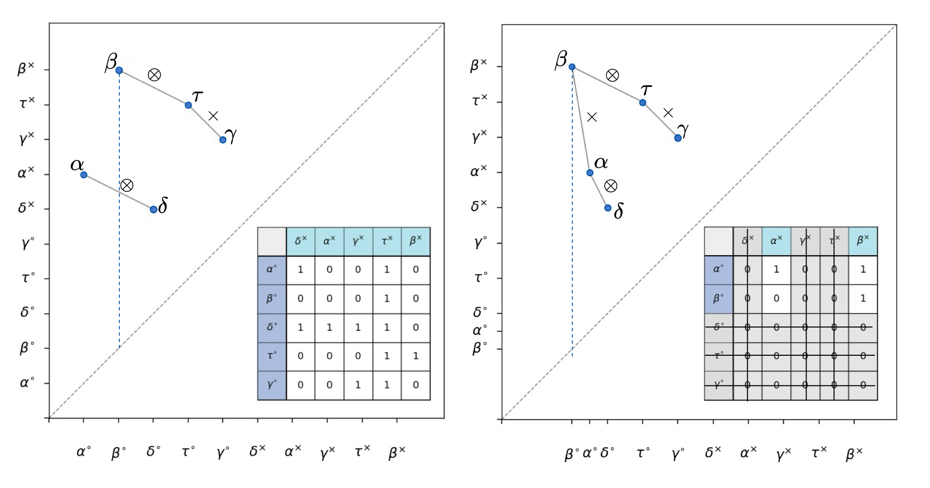
Let be a combinatorial vector field on and let be such that . Assume that there exists a unique path from to . Then is isomorphic to the quotient of after cancelling the pair . (See example in Figure 1.)
So to find a topological simplification of , one can find a critical shallow pair that is reversible. Then, one has to invert the unique path between and , and find with the property that and . Unfortunately, it may happen that there is no pair that is both shallow and reversible. One of the goals of this paper is to remedy this problem.
3 Homology and cohomology relations in the filter
To understand how birth-death pairs and the relationships between them change during changes of the dMf, one must study how they change upon transposition of two adjacent cells in the boundary matrix. This problem is well-studied; see [5] and [13]. Observing that the depth poset can be constructed from the union of homological and cohomological relations between birth-death pairs (see Theorem 4.8 in [12]), we reformulate the results from [13] in the language of this paper. First, we introduce two additional objects.
Lemma 17 ([13, Lemma 3.2]).
Fix a birth-death pair . If we remove all birth-death pairs below and to the right of – in the region – by iteratively canceling shallow pairs, we get the same boundary matrix regardless of the order of cancellations.
Lemma 3 proves that the following definition is unambiguous.
Definition 18.
Fix such that the components of these pairs are consecutive columns in or in . Define to be the matrix obtained by performing Lefschetz cancellations, always canceling shallow pairs, for all pairs lying in the bottom-right quadrant of (excluding if it eventually lies in this region) and for all pairs lying in the bottom-right quadrant of (excluding if it eventually lies in this region).
Note that in the above definition, we can cancel all pairs in the bottom-right quadrants because, from Observation 2, there is no such that . After the cancellations, we have either (i) both and are shallow, or (ii) and is shallow, or (iii) and is shallow.
Now we are ready to utilize results from [13] in a series of theorems.
Theorem 19 (Result of death-cells transposition [13, Lemma 3.4]).
Let be -dimensional birth-death pairs such that . Then the transposition of and does not change the values in , while the changes in follow these rules:
-
(1)
If and , then the pairing is unaffected and the row of the matrix changes according to the formula:
(1) -
(2)
If , then the pairs turn into and and changes as in (1).
-
(3)
Otherwise, and the pairing remain unchanged.
Theorem 20 (Result of birth-cells transposition [13, Lemma 3.3]).
Let and be -dimensional birth-death pairs such that . Then the transposition of and does not change the values in , while the changes in follow these rules:
-
(1)
If and , then the pairing is unaffected and the row of the matrix changes according to the formula:
(2) -
(2)
If , then changes as in (2), and pairs turn into and .
-
(3)
Otherwise and the pairing remain unchanged.
Theorem 21 (Result of birth-death transposition [13, Lemma 3.5]).
A transposition between a birth and a death cell, which is a result of increasing birth, or decreasing death does not affect pairing or relations between birth-death pairs.
Figure 2 presents an example of how a transposition affects the relationship between birth-death pairs. Now we introduce our own propositions, which will be useful later.
Proposition 22.
Fix a pair . A transposition that increases the value of or decreases the value of and does not cause a switch cannot create a relation for any pair .
Note that a transposition may involve skipping two columns and rows when bypassing a combinatorial vector. The following proposition helps decrease complexity of the final algorithm.
Proposition 23.
Let be two dMfs such that and the difference between -order and -order is a transposition between a critical cell and a vector. Then and generate the same off-diagonal birth-death pairs and relations between them.
Proof.
As this process does not change the (co)boundary matrix of , it cannot change the pairing or relations between critical cells.
Finally, the following two corollaries give us an opportunity to focus only on specific cases during the construction of the homotopy below.
Corollary 24.
Take a pair . If is a cell such that and also , then is an -dimensional birth cell. Analogously, if and , then is an -dimensional death cell.
Proof.
Because , the column indexed by was added to column during the lazy reduction of matrix . Because lazy reduction never adds zero columns, column in has a unique low, so it is a death cell. Analogously, if , then column was added to column in , so is a birth cell.
4 Constructing the homotopy
4.1 Homotopy
Recall that a linear homotopy between two maps and is a family of maps for .
We say that is connected if it Hasse diagram – the graph whose vertices are the cells of with an edge for every boundary relation – is connected. An -induced partition is a partition of into maximal, with respect to inclusion, sets , such that is constant on , and every is connected.
Theorem 25.
Let and be two dMfs defined on such that . Let be the linear homotopy between and . Let denote the -induced partition of . Then, for every .
Using this theorem, we can represent our homotopy as a finite series of transpositions, allowing us to analyze only a finite number of time steps. Indeed, along a homotopy there are only finitely many parameters at which fails to be a dMf. On each open interval between two such parameters, the induced -order is well-defined and remains constant (in particular, it does not depend on ). Consequently, for a sufficiently fine discretization of , consecutive -orders differ by exactly one transposition.
4.2 Journey to the diagonal
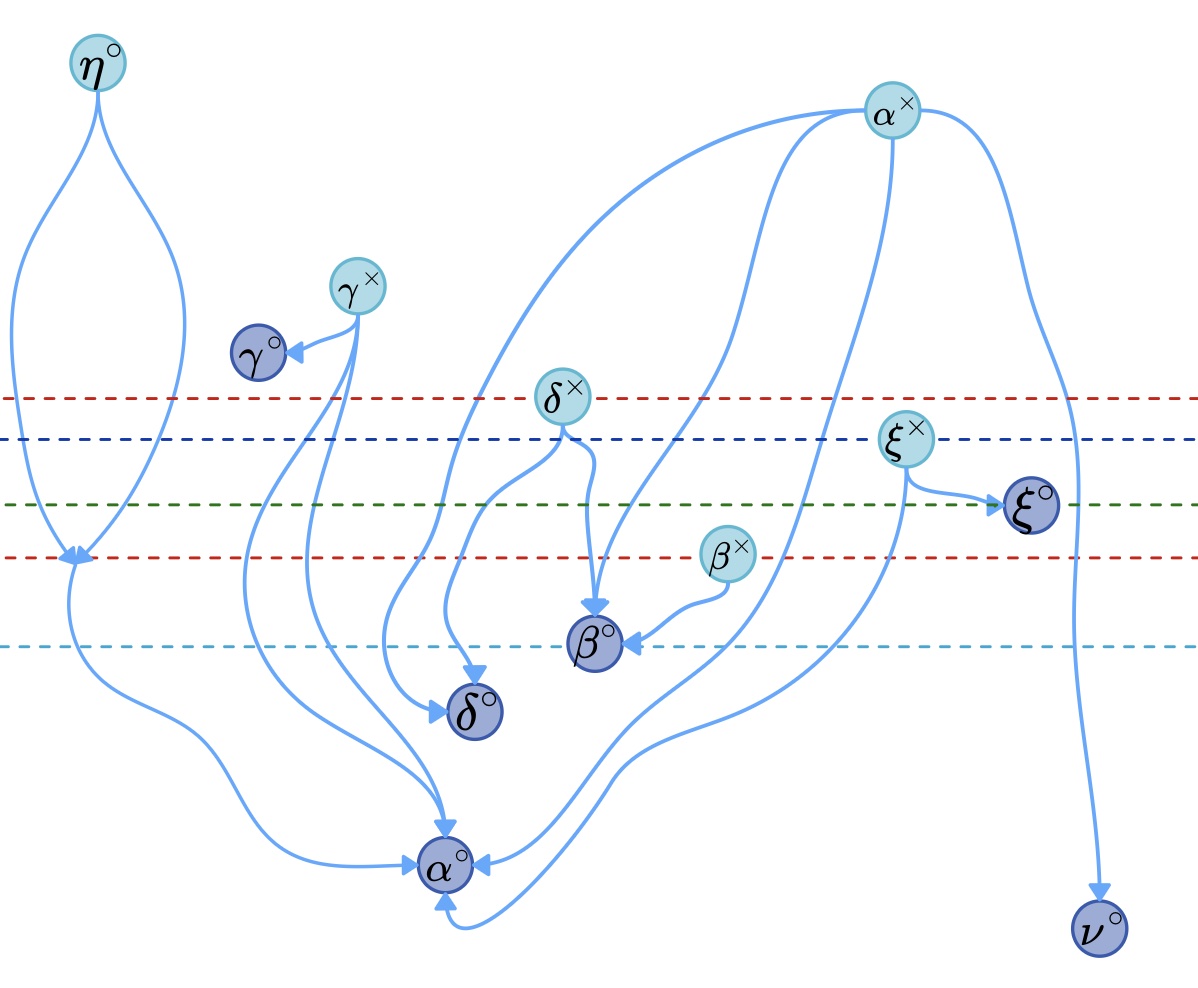
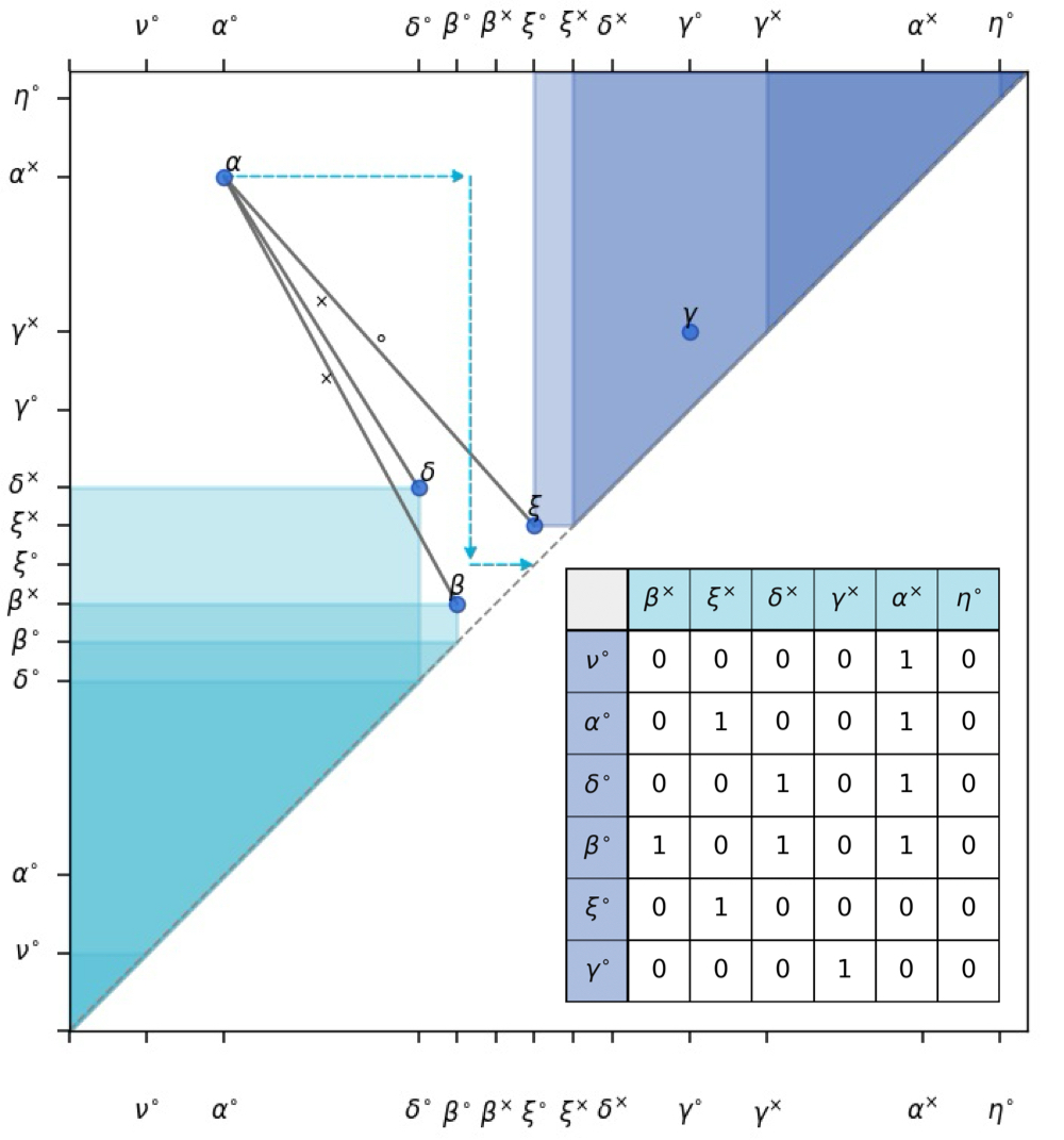
Consider an example in Figure 3 and assume that our goal is to reduce the lifetime of the pair to be arbitrarily small, without changing the pairing or the vector field. To reduce the lifetime, we may increase the value of and decrease the value of , along with a set of vectors. We may implement this as a series of “moves” of the birth-death pair to the right and down in the persistence diagram.
Unfortunately, our moves are constrained: if we want to preserve the original vector field, then we cannot decrease below as , and similarly, cannot increase above . Moreover, as and , we also cannot decrease below these levels, without switches in pairing. Even worse, because , cannot increase above without another switch.
This appears to be a serious obstacle. However, when we examine the persistence diagram (see bottom part of the Figure 3), we notice, following Observation 2, that increasing above breaks both homological relations of without changing the pairing. Afterwards, we are able to decrease as close to as we want. This motivates our central notion of forbidden regions, which describe the allowed “moves” in the persistence diagram.
Definition 26 (Forbidden regions).
For an off-diagonal pair , we say that:
-
(1)
Forbidden region for is defined as
-
(2)
Forbidden region for is defined as
Once we have the notion of forbidden regions, we can define a set of safe transformations, which we call allowed moves.
Definition 27 (Allowed moves).
Let be a dMf, and . A pre-allowed move of is a new dMf such that:
-
(1)
and for all we have ,
-
(2)
If is a birth cell, then ; if is a death cell, then ,
-
(3)
-order and -order restricted to differ by a single transposition at most.
If a pre-allowed move is such that , then we say that is an allowed move.
A pre-allowed move pushes the pair containing toward the diagonal either by increasing birth or decreasing death without affecting the vector field. A single pre-allowed move bypasses at most one other critical cell. We note that multiple vectors can change their value and position in the -order – as long as the gradient structure is preserved. We will use the allowed moves to construct the homotopy bringing a persistent pair to the diagonal.
Corollary 28.
If is a pre-allowed move for , then the change in persistence pairing can only result from transpositions of critical cells.
Proof.
The linear homotopy from to may be expressed as a series of transpositions in -order, given by specific times and -orders. By Theorem 25, the transpositions do not change the vector field, and thus, the diagonal pairs. Therefore, by Proposition 3, the change in persistence pairing can only result from transpositions of critical cells.
Observe that for an filtered by , for every cell and interval such that , we can find such that . We call it the linear coefficient of on . We now show that, for a fixed , one can construct a pre-allowed move that pushes the chosen birth-death pair to the right, and another one that pushes it downward.
Proposition 29 (Increasing birth – moving right).
Let be filtered by a dMf . Let be an off-diagonal pair, and be real values such that , and there is at most one such that . Additionally, assume that and . Define
where is the linear coefficient of on the interval . Then is a pre-allowed move of with respect to .
Proposition 30 (Decreasing death – moving down).
Let be filtered by . Let be an off-diagonal pair, and be real values such that , and there is at most one such that . Additionally, assume and at the same time . Define
where is the linear coefficient of on the interval . Then is a pre-allowed move of with respect to .
Now observe that an allowed move of does not introduce new forbidden regions.
Lemma 31.
Let be an allowed move of . Then and .
Proof.
The statement follows directly from Proposition 3 and the fact that , and we are changing the value of only one component of .
It follows that if we know the initial forbidden regions, we can design a sequence of allowed moves that brings arbitrarily close to the diagonal.
Theorem 32.
Let be filtered by a dMf and be such that , then there exists a sequence of dMfs such that is an allowed move of , and is arbitrarily small.
Proof.
We begin by showing that we are able to construct from an allowed move such that and are closer in -order than in -order, where both orders are restricted to the critical cells. Due to Corollary 4.2, to show that , we can focus only on transpositions between critical cells. Define and as critical cells such that in -order, we have .
If , then if is a death cell or , we use Proposition 4.2 to construct , which increases the value of with the values of and in the proposition larger than . Analogously, if , then if is a birth cell or , then use Proposition 4.2 to construct , which decreases the value of to bypass . From Theorems 19, 20 and 21, we get that these are indeed allowed moves.
If and , then generates forbidden regions bounded by a vertical line and generates forbidden region bounded by a horizontal line. Because , they intersect. We get the same argument if and , or and . If and , then due to Corollary 3, there has to exist . It follows from Observation 2 that they are in the bottom-right quadrant of the pair . Therefore, they generate forbidden and regions, which intersect.
It follows from Lemma 4.2 that if , then .
Accordingly, we can construct a series of allowed moves, such that is the last one, and and are consecutive in the -order restricted to the critical cells. Then, by Proposition 4.2, we construct a final pre-allowed move such that the value gap between the cells of can be made arbitrarily small. Since no critical cell is bypassed during this deformation, the move is allowed.
4.3 Reversing the path
In the previous subsection, we showed that if the forbidden regions of the birth and the death cell of a (reversible) pair do not intersect, then we can reduce its lifetime arbitrarily close to zero. In particular, we can make it a critical shallow pair. It follows from Theorem 16 that we can safely – that is, without introducing changes in the pairing or in the relations – reverse the path between the components of . The reversal is the final step of the construction, which corresponds to entering the diagonal. To make the homotopy fully explicit we construct the final dMf inducing the vector field with reversed path.
Proposition 33.
Let be a reversible pair such that the unique path between and is . If , then the function , defined as
is a dMf which generates and does not change the value of the critical cells other than the components of .
5 Final algorithm and summary
5.1 Final algorithm
We summarize the entire construction in the form of an algorithm that produces a topological simplification of a given dMf.
Input.
A Lefschetz complex filtered by a dMf ; the combinatorial vector field ; the set of birth–death pairs; all homology/cohomology relations among the off-diagonal pairs; and a reversible, -dimensional birth-death pair , such that
- (1)
-
(2)
Reverse the path between and in the vector field, constructing a new dMf as described in Proposition 4.3.
Output.
A Lefschetz complex filtered by a dMf ; the combinatorial vector field ; the set of birth-death pairs; all homology/cohomology relations among the off-diagonal pairs.
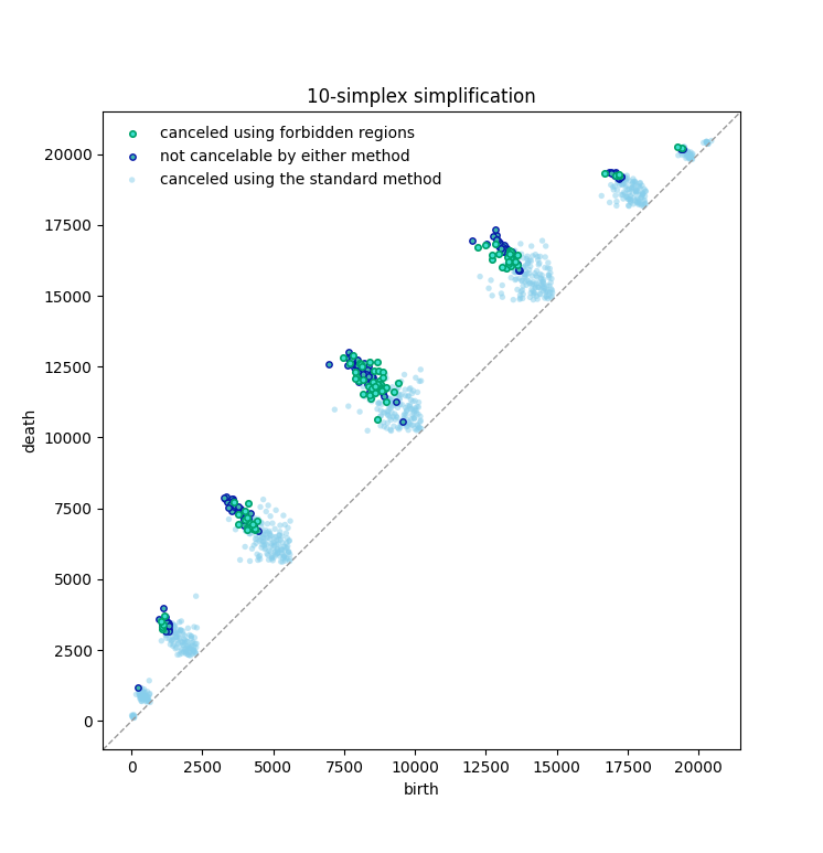
Figure 4 illustrates an example of a topological simplification obtained by this procedure.
Theorem 34.
The algorithm above returns a topological simplification for a dMf . Moreover, the output of the algorithm contains the updated vector field and homology/cohomology relations for .
Proof.
We start by showing that . Step 1 does not cause any changes in the pairing by Theorem 32. A dMf constructed in Step 2 has the same off-diagonal pairs as the previous one, except , due to Theorem 16 and Theorem 12.
Proposition 3 and Theorem 16 imply that it suffices to apply the update pattern and check its conditions only during transpositions of critical cells in Step 1. This results in the updated relations among critical cells at the end of the algorithm.
After the update, the new vector field , where is a unique path. We know the birth-death pairs , as well as all relations between critical cells after the application of the update patterns.
The proof of Theorem 34 also proves Theorem 1. For an iterative execution of the algorithm, we can use its output as an input for the next run; one only needs to provide the next eligible pair. Finally, we consider how much the new constructed dMf differs from the original one.
Proposition 35.
Let be filtered by a dMf , and be its topological simplification constructed by our algorithm, which removes pair . Then, the difference between and is bounded by the lifetime of , that is .
Proof.
It follow directly from the fact that in Propositions 4.2, 4.2 and 4.3, we change only the values of the cells between and , and if the value of the dMf is changed on , then the resulting value also lies between and .
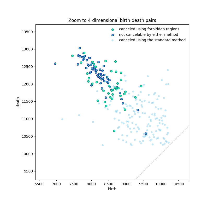
5.2 Complexity
We note that checking if a pair can serve as an input to the algorithm takes time, see [23]; there are at most such pairs to check. The complexity of the algorithm is dominated by the cost of checking if moving pair past pair requires updating relations between birth-death pairs, whenever . Computing can clearly be done in time; however, in the full version of the paper (see [23]) we show that it can be reduced to . Therefore, the worst case running time is , where is the number of birth-death pairs, and is the number of cells in the complex.
5.3 Summary
We presented a new criterion for removing a fixed birth-death pair. We have also shown that for every pair that satisfies this criterion, it is possible to construct a homotopy, which moves this pair into the diagonal. The paper opens a number of questions.
-
(1)
How does the order of cancellations affect the possibility of canceling the remaining pairs? Is there an optimal order? Can we find a hierarchy of cancellations using this order?
-
(2)
Is the criterion exhaustive? That is, are there other removable pairs that are not captured by the criterion?
-
(3)
Is it possible to weaken the criterion by proper manipulation of the pairs generating the forbidden regions? For example, if forbidden region of and forbidden region of intersect, is it possible to manipulate other cells to clear a path to the diagonal for , and restore their values after the cancellation?
-
(4)
Is it possible to parallelize the cancellation process? If so, for which pairs?
References
- [1] Dominique Attali, Marc Glisse, Samuel Hornus, Francis Lazarus, and Dmitriy Morozov. Persistence-sensitive simplification of functions on surfaces in linear time. Manuscript, presented at TOPOINVIS, 9:23–24, 2009.
- [2] Ulrich Bauer. Ripser: efficient computation of Vietoris–Rips persistence barcodes. Journal of Applied and Computational Topology, 5(3):391–423, 2021. doi:10.1007/s41468-021-00071-5.
- [3] Ulrich Bauer, Carsten Lange, and Max Wardetzky. Optimal topological simplification of discrete functions on surfaces. Discrete & Computational Geometry, 47(2):347–377, 2012. doi:10.1007/s00454-011-9350-z.
- [4] Ulrich Bauer and Fabian Roll. Wrapping Cycles in Delaunay Complexes: Bridging Persistent Homology and Discrete Morse Theory. In Wolfgang Mulzer and Jeff M. Phillips, editors, 40th International Symposium on Computational Geometry (SoCG 2024), volume 293 of Leibniz International Proceedings in Informatics (LIPIcs), pages 15:1–15:16, Dagstuhl, Germany, 2024. Schloss Dagstuhl – Leibniz-Zentrum für Informatik. doi:10.4230/LIPIcs.SoCG.2024.15.
- [5] David Cohen-Steiner, Herbert Edelsbrunner, and Dmitriy Morozov. Vines and vineyards by updating persistence in linear time. In Proceedings of the Twenty-Second Annual Symposium on Computational Geometry (SoCG’06), pages 119–126. ACM, 2006. doi:10.1145/1137856.1137877.
- [6] Lidija Comic and Leila De Floriani. Cancellation of critical points in 2d and 3d morse and morse-smale complexes. In David Coeurjolly, Isabelle Sivignon, Laure Tougne, and Florent Dupont, editors, Discrete Geometry for Computer Imagery, 14th IAPR International Conference, DGCI 2008, Lyon, France, April 16-18, 2008. Proceedings, volume 4992 of Lecture Notes in Computer Science, pages 117–128, Berlin, Heidelberg, 2008. Springer. doi:10.1007/978-3-540-79126-3_12.
- [7] Lidija Comic, Leila De Floriani, Federico Iuricich, and Paola Magillo. Computing a discrete morse gradient from a watershed decomposition. Comput. Graph., 58:43–52, 2016. doi:10.1016/j.cag.2016.05.020.
- [8] Vin de Silva, Dmitriy Morozov, and Mikael Vejdemo-Johansson. Dualities in persistent (co)homology. Inverse problems, 27(12):124003, November 2011. doi:10.1088/0266-5611/27/12/124003.
- [9] Olaf Delgado-Friedrichs, Vanessa Robins, and Adrian Sheppard. Skeletonization and partitioning of digital images using discrete Morse theory. IEEE Trans Pattern Anal Mach Intell, 37(3):654–666, March 2015. doi:10.1109/TPAMI.2014.2346172.
- [10] Tamal K. Dey, Jiayuan Wang, and Yusu Wang. Improved road network reconstruction using discrete Morse theory. In Proceedings of the 25th ACM SIGSPATIAL International Conference on Advances in Geographic Information Systems (SIGSPATIAL ’17), pages 58:1–58:4, New York, NY, USA, 2017. ACM. doi:10.1145/3139958.3140031.
- [11] Herbert Edelsbrunner, David Letscher, and Afra Zomorodian. Topological persistence and simplification. Discrete & Computational Geometry, 28(4):511–533, 2002. doi:10.1007/s00454-002-2885-2.
- [12] Herbert Edelsbrunner, Michał Lipiński, Marian Mrozek, and Manuel Soriano Trigueros. The poset of cancellations in a filtered complex. arXiv:2311.14364v3, 2024. arXiv:2311.14364.
- [13] Herbert Edelsbrunner, Michał Lipiński, Marian Mrozek, Manuel Soriano Trigueros, and Fedor Zimin. The depth poset under transpositions in the filter. arXiv:2511.21961, 2025. doi:10.48550/arXiv.2511.21961.
- [14] Herbert Edelsbrunner, Dmitriy Morozov, and Valerio Pascucci. Persistence-sensitive simplification functions on 2-manifolds. In Proceedings of the Twenty-second Annual Symposium on Computational Geometry, SCG ’06, pages 127–134, New York, NY, USA, 2006. ACM. doi:10.1145/1137856.1137878.
- [15] Herbert Edelsbrunner and Marian Mrozek. The depth poset of a filtered Lefschetz complex. arXiv:2311.14364v2, 2023. doi:10.48550/arXiv.2311.14364.
- [16] Riccardo Fellegara, Federico luricich, Leila De Floriani, and Kenneth Weiss. Efficient computation and simplification of discrete Morse decompositions on triangulated terrains. In Proceedings of the 22nd ACM SIGSPATIAL International Conference on Advances in Geographic Information Systems, SIGSPATIAL ’14, pages 223–232, New York, NY, USA, 2014. Association for Computing Machinery. doi:10.1145/2666310.2666412.
- [17] Robin Forman. Combinatorial vector fields and dynamical systems. Mathematische Zeitschrift, 228(4):629–681, 1998. doi:10.1007/PL00004638.
- [18] Robin Forman. Morse theory for cell complexes. Advances in Mathematics, 134(1):90–145, 1998. doi:10.1006/aima.1997.1650.
- [19] Robin Forman. A user’s guide to discrete Morse theory. Séminaire Lotharingien de Combinatoire [electronic only], 48:B48c, 35 p., electronic only–B48c, 35 p., electronic only, 2002. URL: http://eudml.org/doc/123837.
- [20] Rickard Brüel Gabrielsson, Vignesh Ganapathi-Subramanian, Primoz Skraba, and Leonidas J. Guibas. Topology-aware surface reconstruction for point clouds. Comput. Graph. Forum, 39(5):197–207, 2020. doi:10.1111/cgf.14079.
- [21] David Günther, Jan Reininghaus, Hubert Wagner, and Ingrid Hotz. Efficient computation of 3D Morse–Smale complexes and persistent homology using discrete Morse theory. The Visual Computer, 28(10):959–969, 2012. doi:10.1007/s00371-012-0726-8.
- [22] Attila Gyulassy, Peer-Timo Bremer, Bernd Hamann, and Valerio Pascucci. A practical approach to Morse-Smale complex computation: Scalability and generality. IEEE Transactions on Visualization and Computer Graphics, 14(6):1619–1626, 2008. doi:10.1109/TVCG.2008.110.
- [23] Jakub Leśkiewicz, Bartosz Furmanek, Michał Lipiński, and Dmitriy Morozov. Topological simplification guided by forbidden regions, 2026. doi:10.48550/arXiv.2603.16416.
- [24] John Milnor. Morse Theory. Princeton University Press, 1963.
- [25] John Milnor. Lectures on the h-Cobordism Theorem. Princeton University Press, 1965.
- [26] Arnur Nigmetov and Dmitriy Morozov. Topological optimization with big steps. Discrete & Computational Geometry, 72:310–344, 2024. doi:10.1007/s00454-023-00613-x.
- [27] Vanessa Robins, Peter John Wood, and Adrian P. Sheppard. Theory and algorithms for constructing discrete Morse complexes from grayscale digital images. IEEE Transactions on Pattern Analysis and Machine Intelligence, 33(8):1646–1658, 2011. doi:10.1109/TPAMI.2011.95.