Manifolds of Positive Reach, Differentiability, Tangent Variation, and Attaining the Reach

Consider a topologically embedded manifold with positive reach. That is, we don’t assume anything on the embedding of the manifold except that it is a homeomorphism with its image. However, the assumption that the manifold has positive reach yields that the generalized tangent spaces (see Definition 7) are cones.

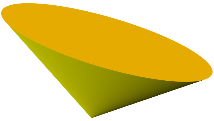
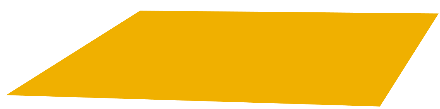
We characterize convex cones by topological means (roughly speaking) as follows. We recall that a convex cone is a subset of ${ℝ}^d$ that is convex and for each $v$ in the set we have that $\lambda v$ is also in the set for $\lambda \in {ℝ}_{\ge 0}$. By this we mean that, roughly speaking, convex cones $A$ come into two classes:

1. 1.

   The convex cone is defined by

   $$A=\{\lambda a|\lambda \ge 0,a\in \tilde{A}\},$$

   where $\tilde{A}$ is a contractible subset of ${𝕊}^{d-1}$. Note that $\tilde{A}=A\cap {𝕊}^{d-1}$. In this case $A$ is (again roughly speaking) either a tapering object or a half space.

2. 2.

   The convex cone is defined by

   $$A=\{\lambda a|\lambda \ge 0,a\in \tilde{A}\},$$

   where $\tilde{A}$ is a ($k$ dimensional, with $0\le k\le d-1$) geodesic sphere in ${𝕊}^{d-1}$. In this case $A$ is a vector space.

These two classes are characterized by the homology of $B(0,1)\setminus A^{⟂}$. The contractibility of $\tilde{A}$ is the key ingredient, see Lemma 30 of [20]. More precisely, we’ll use that $\tilde{A}$ is contractible on the sphere if and only if $A$ isn’t a vector space.

In Section A.2 of the appendix of [20] we’ll establish, based on the characterization of Appendix A.1 of [20], that for topologically embedded manifolds the tangent cones are in fact tangent spaces. The proof proceeds in two steps:

• $\mathrm{■}$

  In Lemma 31 of [20], we’ll see that $B(p,\rho )\setminus \left(p+\mathrm{Nor}(p,𝒮)\right)$ has the same homology as $𝒮\cap B(p,\rho )\setminus \{p\}$, see Figure 3. This result will rely on the deformation retract along the closest point projection of sets of positive reach and its continuity as established by Federer [13]. We stress that the normal cone $\mathrm{Nor}(p,𝒮)$ is the dual of the tangent cone $\mathrm{Tan}(p,𝒮)$, which explains the link with Lemma 30 of [20].

• $\mathrm{■}$

  In the proof of Lemma 32 of [20], we’ll see that if $ℳ$ is manifold, then $ℳ\cap B(p,\rho )\setminus \{p\}$ has the homology of a sphere of dimension $n-1$, which with the previous lemma allows us to conclude that $\mathrm{Tan}(p,ℳ)$ is a vector space. The proof combines topological reasoning with arguments based on the charts of the manifold $ℳ$.

By definition we have that if a manifold has a tangent space it is differentiably embedded, but that does not mean that the manifold has to be continuously differentiably embedded, this is what will be the topic we’ll address next.

In Section A.3 of [20] we will first prove a more general statement (Lemma 33 of [20]), namely semi-continuity of the normal cones for general sets of positive reach. By this we mean that given a point $p$ and its normal cone $\mathrm{Nor}(p,𝒮)$, for all $ϵ$ there exists a neighbourhood of $p$ such that for all $p^{\prime }$ in this neighbourhood, we have that the normal cone $\mathrm{Nor}(p^{\prime },𝒮)$ makes only an $ϵ$ angle with some subset of $\mathrm{Nor}(p,𝒮)$. The proof is elementary, but rather technical, and relies on compactness arguments and the manipulation of offsets.

Lemma 33 of [20] together with the observation that the tangent spaces are $k$-dimensional vector spaces the one sided bound on the angle between the normal cones above is in fact a two-sided bound, see Lemma 34 of [20], yields that the manifold is $C^1$, that is continuously differentiable. Lemma 35 of [20] strengthens this even further and explains that $ℳ$ can locally be written as the graph of a function. To put it differently, using some geometrical and analytical arguments we see that the manifold (locally) projects injectively on its tangent cone (which is an affine space by Lemma 32 of [20]). This then allows us to identify it, locally, as the graph of a differentiable map from the tangent space to the normal space.

Appendix A.4 of [20] proves the majority of the main statements of the paper, namely that manifolds with positive reach are $C^{1,1}$ and characterizes the Lipschitz constants of the derivative in terms of the local reach. It is the most technical section and relies heavily on the theory of semiconcave functions. Most crucially we’ll use the following result, namely Corollary 3.3.8 of [9]:

Although that the precise technical way that this result is used is too intricate to explain in a paragraph or two, the link between sets of positive reach and Lemma 17 can be explained in geometrical terms. Assume for the moment that $ℳ$ has reach $1$. As a consequence of Lemma 13 the interior of every ball that is tangent to a manifold $ℳ$, that has radius less or equal to $1$ (the reach of $ℳ$) does not intersect $ℳ$ itself. Geometrically speaking the fact that $x\to 1/2x^2-F(x)$ and $x\to 1/2x^2+F(x)$ are convex functions can be expressed by the fact that (locally) the interior of parabolae that are tangent to the manifold have an empty interior, see Figure 4. Of course these parabolae are just second order approximations of the spheres. Because we are just interested in the Lipschitz constants of the derivative this approximation suffices.

Using Lemma 17 we do not directly prove our bound on the angle between nearby tangent spaces, instead we first establish the bound

see Lemma 39 of [20], where $\varphi$ is the local function (from the tangent to normal space) of which $ℳ$ is locally the graph and $\parallel \cdot \parallel$ denotes the operator two norm, in other words we regard the Jacobians as matrices depending on $y$ and bound their Lipschitz constant in a way that is $ϵ$ close to optimal.

From the result of Lemma 39 of [20] it is not very difficult to derive a local bound between tangent spaces, which is done in Lemma 40 of [20]. This local bound can then be extended (Lemma 41 of [20]) to a non-local statement by gluing the local estimates on the angle between tangent spaces along a geodesic, which exists thanks to Lemma 15. This allows us to establish one of the main results, the characterization of the local reach in terms of the tangent variation in Theorem 4, whose proof requires a significant amount of computation. The optimal size of the domain (in a fixed tangent space) such that $ℳ$ can be written as the graph of a function from a (fixed) tangent space to its normal space is then given in Theorem 1. The proof can be sketched as follows: By combining Theorems 4 and 16 with the submersion theorem we can establish a local diffeomorphism. The global diffeomorphism is established by proving that the covering number is one.

By definition of ${\mathrm{rch}}_{loc.}(p,𝒮)$, we have that for any $ϵ>0$ there is $\rho >0$ such that:

One gets

Because this inequality holds for any positive $ϵ$, the equality follows. $◀$

We have the following variant of Lemma 12 of [8], which in turn is a relatively straightforward generalization to arbitrary dimension of Property I of [5]:

The length of $\gamma$ in the direction $\dot{\gamma }(\frac{\mathrm{\ell }}{2})$ is

where, in the above inequality, we use the assumption $\mathrm{\ell }\le 2\pi R$ and the fact that $\theta \mapsto \cos \theta$ is decreasing on $[0,\pi ]$.

Because $|q-p|\ge ⟨q-p,\dot{\gamma }(\frac{\mathrm{\ell }}{2})⟩$, we see that

$◀$

Combining Lemmas 42 of [20] and 21 we get:

The Lemma 23 below is a special case of [19, Lemma 4.6], we still provide a proof for completeness.

Consider the closed set ${𝒮}^{\prime }:=𝒮\setminus B^{\circ }(\tilde{x},ϵ)$. The minimum distance $d(x,{𝒮}^{\prime })$ to $x$ is attained at least at some point $z$ in ${𝒮}^{\prime }$ so that

Taking

we get, for any $y$ such that and $z\in {𝒮}^{\prime }$ that:

We have shown that if $z\in {𝒮}^{\prime }$, then $d(y,z)>d(y,𝒮)$. It follows that any closest point to $y$ in $𝒮$ is in $𝒮\setminus {𝒮}^{\prime }=𝒮\cap B^{\circ }(\tilde{x},ϵ)$ which is (12). $◀$

We consider first the situation where $\mathrm{rch}(𝒮)=0$. In this case, since $𝒮$ is bounded, there exists some point $p\in \overline{\mathrm{ax}(𝒮)}\cap 𝒮$. Then, for any $\rho >0$, there is some $p^{\prime }\in \mathrm{ax}(𝒮)$ such that , so that there are at least two points in $𝒮\cap B(p,\rho )$ closest to $p^{\prime }$. Thus, , and, since this holds for any $\rho >0$, we get that ${\mathrm{rch}}_{loc.}(p,𝒮)=0$ and as a direct consequence ${\mathrm{rch}}_{loc.}(𝒮)={inf}_{q\in 𝒮}{\mathrm{rch}}_{loc.}(q,𝒮)=0$.

We assume now that $\mathrm{rch}(𝒮)>0$.

As we have seen in Equation (4) of Remark 3, we have that $\mathrm{rch}(𝒮)\le {\mathrm{rch}}_{loc.}(𝒮)$. Therefore it suffices to prove that, if , then $\mathrm{rch}(𝒮)={\mathrm{rch}}_{glob.}(𝒮)$. So let us assume now that .

Since $𝒮$ is compact and thus bounded, which implies that a closed $\mathrm{rch}(𝒮)$-neighbourhood of $𝒮$ is also bounded, there must exist $x\in \overline{\mathrm{ax}(𝒮)}$, where $\overline{\mathrm{ax}(𝒮)}$ is the closure of the medial axis $\mathrm{ax}(𝒮)$, such that $d(x,𝒮)=\mathrm{rch}(𝒮)$.

If $x\in \overline{\mathrm{ax}(𝒮)}\setminus \mathrm{ax}(𝒮)$, in particular $x\notin \mathrm{ax}(𝒮)$ and there is a unique point $\tilde{x}$ closest to $x$ in $𝒮$. Choose some and, as in Lemma 23, take $\alpha >0$ so that (12) holds and, moreover, such that

Since $x\in \overline{\mathrm{ax}(𝒮)}$, there exists $y\in \mathrm{ax}(𝒮)\cap B^{\circ }(x,\alpha ))$, and therefore Lemma 23 yields that there exists at least two points $p,q\in B^{\circ }(\tilde{x},ϵ)$ such that $d(y,p)=d(y,q)=d(y,𝒮)$.

Because , by Theorem 16, there is a geodesic from $p$ to $q$ of length at most $\pi \mathrm{rch}(𝒮)$, which is less that $2\pi {\mathrm{rch}}_{loc.}(𝒮)$. But then one can apply Corollary 22, which implies that the length of a geodesic from $p$ to $q$ is at most

However, since projecting a curve outside a given sphere onto the given sphere only decreases its length, a curve from $p$ to $q$ outside the ball centered at $y$ whose radius is at most must have length strictly greater than ${\mathrm{\ell }}_{\max }$, a contradiction.

We have so far proven that when , then the reach cannot be realized in $\overline{\mathrm{ax}(𝒮)}\setminus \mathrm{ax}(𝒮)$. One must then have $x\in \mathrm{ax}(𝒮)$ and there are at least two points $p\ne q$ closest points to $x$ on $𝒮$.

If then by Theorem 16 one has that $d_{𝒮}(p,q)\le 2\mathrm{r}\mathrm{c}\mathrm{h}(𝒮)\arcsin \frac{|p-q|}{2\mathrm{r}\mathrm{c}\mathrm{h}(𝒮)}$ which is less than $2\pi {\mathrm{rch}}_{loc.}(𝒮)$. Again, Corollary 22 implies that the length of a geodesic from $p$ to $q$ is a most $2\mathrm{r}\mathrm{c}{\mathrm{h}}_{loc.}(𝒮)\arcsin \frac{|p-q|}{2\mathrm{r}\mathrm{c}{\mathrm{h}}_{loc.}(𝒮)}$, which, again, is impossible without entering the ball centered at $x$ with radius .

Since $|p-q|\le 2\mathrm{r}\mathrm{c}\mathrm{h}(𝒮)$, the only possibility is that $|p-q|=2\mathrm{r}\mathrm{c}\mathrm{h}(𝒮)$, i.e. $x=(p+q)/2$, a bottleneck. $◀$

References

- [1] Eddie Aamari, Jisu Kim, Frédéric Chazal, Bertrand Michel, Alessandro Rinaldo, and Larry Wasserman. Estimating the reach of a manifold. Electronic journal of statistics, 13(1):1359–1399, 2019.
- [2] Eddie Aamari and Clément Levrard. Stability and minimax optimality of tangential Delaunay complexes for manifold reconstruction. Discrete & Computational Geometry, 59(4):923–971, 2018. doi:10.1007/s00454-017-9962-z.
- [3] Naum Il’ich Akhiezer and Izrail Markovich Glazman. Theory of linear operators in Hilbert space. Courier Corporation, 2013.
- [4] N. Amenta and M. Bern. Surface reconstruction by Voronoi filtering. Discrete & Computational Geometry, 22(4):481–504, December 1999. doi:10.1007/PL00009475.
- [5] Dominique Attali, Herbert Edelsbrunner, and Yuriy Mileyko. Weak Witnesses for Delaunay triangulations of Submanifold. In ACM Symposium on Solid and Physical Modeling, pages 143–150, Beijing, China, June 2007. doi:10.1145/1236246.1236267.
- [6] Dominique Attali and André Lieutier. Geometry-driven collapses for converting a Čech complex into a triangulation of a nicely triangulable shape. Discrete & Computational Geometry, 54(4):798–825, 2015. doi:10.1007/S00454-015-9733-7.
- [7] Jean-Daniel Boissonnat, Frédéric Chazal, and Mariette Yvinec. Geometric and Topological Inference. Cambridge Texts in Applied Mathematics. Cambridge University Press, 2018. doi:10.1017/9781108297806.
- [8] Jean-Daniel Boissonnat, André Lieutier, and Mathijs Wintraecken. The reach, metric distortion, geodesic convexity and the variation of tangent spaces. Journal of Applied and Computational Topology, 3(1):29–58, June 2019. doi:10.1007/s41468-019-00029-8.
- [9] Piermarco Cannarsa and Carlo Sinestrari. Semiconcave functions, Hamilton-Jacobi equations, and optimal control, volume 58. Springer Science & Business Media, 2004.
- [10] S.-W. Cheng, T.K. Dey, and J.R. Shewchuk. Delaunay Mesh Generation. Computer and information science series. CRC Press, 2013.
- [11] Robert J Daverman and Gerard Venema. Embeddings in manifolds, volume 106. American Mathematical Soc., 2009.
- [12] T.K. Dey. Curve and Surface Reconstruction: Algorithms with Mathematical Analysis. Number 23 in Cambridge monographs on applied and computational mathematics. Cambridge University Press, 2007.
- [13] H. Federer. Curvature measures. Transactions of the American mathematical Society, 93:418–491, 1959.
- [14] Charles Fefferman, Sergei Ivanov, Yaroslav Kurylev, Matti Lassas, and Hariharan Narayanan. Reconstruction and interpolation of manifolds. I: The geometric Whitney problem. Foundations of Computational Mathematics, 2019. doi:10.1007/s10208-019-09439-7.
- [15] Charles Fefferman, Sergei Ivanov, Matti Lassas, and Hariharan Narayanan. Fitting a manifold of large reach to noisy data. arXiv e-prints, page arXiv:1910.05084, October 2019. arXiv:1910.05084.
- [16] Tosio Kato. Perturbation theory for linear operators, volume 132. Springer Science & Business Media, 2013.
- [17] Marc Khoury and Jonathan Richard Shewchuk. Approximation bounds for interpolation and normals on triangulated surfaces and manifolds. arXiv preprint arXiv:1911.03424, 2019. arXiv:1911.03424.
- [18] Gunther Leobacher and Alexander Steinicke. Existence, uniqueness and regularity of the projection onto differentiable manifolds. Annals of Global Analysis and Geometry, 60(3):559–587, July 2021. doi:10.1007/s10455-021-09788-z.
- [19] André Lieutier. Any open bounded subset of has the same homotopy type as its medial axis. Computer-Aided Design, 36(11):1029–1046, 2004. Solid Modeling Theory and Applications. doi:10.1016/j.cad.2004.01.011.
- [20] André Lieutier and Mathijs Wintraecken. Manifolds of positive reach, differentiability, tangent variation, and attaining the reach. Full version, 2026. URL: https://inria.hal.science/hal-04816588.
- [21] Alexander Lytchak. On the geometry of subsets of positive reach. manuscripta mathematica, 115(2):199–205, 2004.
- [22] Alexander Lytchak. Almost convex subsets. Geometriae Dedicata, 115(1):201–218, 2005.
- [23] K. Menger. Untersuchungen über allgemeine Metrik. Vierte Untersuchung. Zur Metrik der Kurven. Mathematische Annalen, 103:466–501, 1930.
- [24] P. Niyogi, S. Smale, and S. Weinberger. Finding the homology of submanifolds with high confidence from random samples. Discrete & Computational Geometry, 39(1-3):419–441, 2008. doi:10.1007/S00454-008-9053-2.
- [25] Li Qiu, Yanxia Zhang, and Chi-Kwong Li. Unitarily invariant metrics on the grassmann space. SIAM Journal on Matrix Analysis and Applications, 27(2):507–531, 2005. doi:10.1137/040607605.
- [26] Jan Rataj and Luděk Zajíček. On the structure of sets with positive reach. Mathematische Nachrichten, 290(11-12):1806–1829, 2017.
- [27] S. Scholtes. On hypersurfaces of positive reach, alternating Steiner formulae and Hadwiger’s Problem. ArXiv e-prints, April 2013. arXiv:1304.4179.
- [28] Barak Sober and David Levin. Manifold approximation by moving least-squares projection (MMLS). Constructive Approximation, pages 1–46, 2019. doi:10.1007/s00365-019-09489-8.
- [29] Yuan Wang and Bei Wang. Topological inference of manifolds with boundary. Computational Geometry, 88:101606, 2020. doi:10.1016/j.comgeo.2019.101606.
- [30] Per Åke Wedin. On angles between subspaces of a finite dimensional inner product space. In Matrix Pencils: Proceedings of a Conference Held at Pite Havsbad, Sweden, March 22–24, 1982, pages 263–285. Springer, 2006.
- [31] Yung-Chow Wong. Differential geometry of Grassmann manifolds. Proceedings of the National Academy of Sciences of the United States of America, 57(3):589, 1967.