The Voronoi Diagram of Four Lines in ℝ³

Papadopoulou, Evanthia; Wang, Zeyu

doi:10.4230/LIPIcs.SoCG.2026.84

The Voronoi Diagram of Four Lines in $\mathbb{R}^{3}$

Evanthia Papadopoulou

Faculty of Informatics, Università della Svizzera italiana (USI), Lugano, Switzerland Zeyu Wang

Faculty of Informatics, Università della Svizzera italiana (USI), Lugano, Switzerland

Abstract

We consider the Voronoi diagram of lines in $\mathbb{R}^{3}$ under the Euclidean metric, and give a full classification of its structure in the base case of four lines in general position. We first show that the number of vertices in the Voronoi diagram of four lines in general position is always even, between 0 and 8, and all such numbers can be realized. We identify a key structure for the diagram formation, called a twist, which is a pair of consecutive intersections among trisector branches; only two types of twists are possible, so-called full and partial twists. A full twist is a purely local structure, which can be inserted or removed without affecting the rest of the diagram. Assuming no full twists, the nearest and the farthest Voronoi diagrams of four lines, each have 15 distinct topologies, which are in one-to-one correspondence; the two-dimensional faces are all unbounded, and the total number of vertices is at most six. The unbounded features of the farthest diagram, encoded in a two-dimensional spherical map, are also in one-to-one correspondence. The identified topologies are all realizable. Any Voronoi diagram of four lines in general position in $\mathbb{R}^{3}$ can be obtained from one of these topologies by inserting full twists; each twist induces a bounded face of exactly two vertices in both the nearest and farthest diagrams. We obtain the classification by an exhaustive search algorithm using some new structural and combinatorial observations of line Voronoi diagrams.

Keywords and phrases:

Voronoi diagram, lines, three dimensions, structural properties

Copyright and License:

2012 ACM Subject Classification:

Theory of computation

\rightarrow

Computational geometry

Related Version:

Full Version: https://arxiv.org/abs/2603.19836

Supplementary Material:

Software: https://doi.org/10.5281/zenodo.19090548 [22]

Acknowledgements:

We thank Dr. Martin Suderland for early discussions and valuable comments related to Sections 2, 3, and for two Matlab-based visualisation tools, which allowed us to visualize

\Gamma(\mathrm{FVD}(L))

, Figure 6, and Figure 13. We also thank anonymous reviewers for comments that helped improve the presentation of this paper, the general position assumption, and Lemma 3.

Funding:

Supported by the Swiss National Science Foundation (SNF), project 200021E

\_

201356.

DOI:

10.4230/LIPIcs.SoCG.2026.84

Event:

42nd International Symposium on Computational Geometry (SoCG 2026)

Editors:

Hee-Kap Ahn, Michael Hoffmann, and Amir Nayyeri

Series and Publisher:

Leibniz International Proceedings in Informatics, Schloss Dagstuhl – Leibniz-Zentrum für Informatik

1 Introduction

Voronoi diagrams are fundamental space partitioning structures in Computational Geometry. Given a set $S$ of $n$ objects in some space, called sites, the nearest (respectively, farthest) Voronoi diagram of $S$ decomposes the underlying space into regions that have the same nearest (resp., farthest) site. In this paper, we consider Voronoi diagrams of lines in $\mathbb{R}^{3}$ under the Euclidean metric, focusing on the elementary, yet fundamental base case of four lines.

The Euclidean Voronoi diagram of point sites in $\mathbb{R}^{d}$ is a classical geometric partitioning structure that is generally well-understood. It has complexity $O(n^{\lceil\frac{d}{2}\rceil})$ and can be computed in $O(n\log n+n^{\lceil\frac{d}{2}\rceil})$ time [10, 7, 16]; these bounds are tight. The results also hold for certain polyhedral norms such as the $L_{\infty}$ or $L_{1}$ norms [6, 15]. For the Euclidean farthest Voronoi diagram of point sites, exact worst-case bounds in the range of $\Theta(n^{\lceil\frac{d}{2}\rceil})$ have also been reported by Seidel [20].

For sites more general than points, however, Voronoi diagrams in $\mathbb{R}^{d}$ , $d\geq 3$ , have not yet been well-understood. These diagrams get complicated because their bisecting surfaces are curved, triggering complicated algebraic descriptions of their features such as their trisector curves. The combinatorial complexity of the classical Voronoi diagram of $n$ lines (or line segments) in $\mathbb{R}^{3}$ is a well-known outstanding open problem [19]. There is a gap of an order of magnitude between the $\Omega(n^{2})$ lower bound [2] and the only known $O(n^{3+\varepsilon})$ upper bound by Sharir [21]. This gap extends to the Voronoi diagram of lines in $\mathbb{R}^{d}$ , $d>3$ , where the known upper bound is $O(n^{d+\varepsilon})$ [21]. For $d\geq 4$ , an $\Omega(n^{\lceil 2d/3\rceil})$ lower bound has recently been reported by Glisse [13]. The upper bounds are derived from general complexity results on envelopes of algebraic functions in $\mathbb{R}^{d+1}$ , under the general framework [10] for studying Voronoi diagrams in $\mathbb{R}^{d}$ through the arrangement of distance functions of the given sites in $\mathbb{R}^{d+1}$ . Sharper complexity bounds have been established in certain special cases such as lines with $c$ constant orientations [18] and parallel half-lines [3], and for norms induced by convex polyhedra of constant complexity [8, 17, 4].

The Voronoi diagram of only three lines in $\mathbb{R}^{3}$ was addressed by the authors of [12] who proved the fundamental properties of its structure. The trisector of three pairwise skew lines was shown to consist of four unbounded curves, which are roots of a nonsingular quartic, or a nonsingular cubic and a nonintersecting line. This is the first, most basic building block necessary in computing any Voronoi diagram of lines or polyhedra in $\mathbb{R}^{3}$ , but it contains no Voronoi vertices. In this paper, we address the next basic building block, which is the Voronoi diagram of four lines in $\mathbb{R}^{3}$ , where a minimal number of Voronoi vertices appears.

The unbounded features of the Euclidean order- $k$ , $1\leq k\leq n{-}1$ , Voronoi diagrams of lines and line segments in $\mathbb{R}^{d},d\geq 3$ , were studied in [5]. They are encoded in a map on a sphere of directions, called the Gaussian map, which has complexity $O(\min\{k,n-k\}n^{d-1})$ ; for the farthest Voronoi diagram the Gaussian map has complexity $\Theta(n^{d-1})$ .

The Voronoi diagram of lines in $\mathbb{R}^{3}$ can be computed in $O(n^{3+\epsilon})$ time [1] as part of a more general technique to compute the lower envelope of algebraic functions in $\mathbb{R}^{4}$ . Using the envelope package of CGAL, a numerically robust algorithm for computing the Voronoi diagram of lines in $\mathbb{R}^{3}$ has been reported in [14]. Algorithms for computing approximations of the Voronoi diagram also exist, see e.g., [11, 9].

Contribution.

In this paper, we prove structural properties of the Voronoi diagram of four lines in $\mathbb{R}^{3}$ , building upon the previous work [12] on three lines. The case of four lines is fundamental, and is required for understanding any Voronoi diagram of lines or polyhedra in $\mathbb{R}^{3}$ . We first show that the number of vertices in the Voronoi diagram of four lines in general position is always even, between 0 and 8, and all such numbers can be realized. We then identify basic structures in the arrangement of trisectors, called twists, which are critical for the formation of the diagram and the resulting number of its Voronoi vertices. A twist is a pair of consecutive trisector intersections along some trisector components (called branches, see Definition 10). We show that there are only two types of twists: full twists that involve four different trisector branches, and partial twists that involve six trisector branches, two of which are incident to both vertices of the twist (see Definition 11). A full twist has a local structure, in the sense that adding or removing one does not affect the rest of the diagram. It results in a bounded face with exactly two vertices in both the nearest and the farthest diagrams. Since full twists only have a local effect, we first assume that no full twists exist in the trisector arrangement and fully classify the Voronoi diagrams of four lines in this case. We prove the following theorems.

Theorem 1.

The Voronoi diagram of four lines in general position in $\mathbb{R}^{3}$ (both the nearest and farthest diagram) has 15 distinct topologies, assuming there are no full twists among the trisectors. The distinct topologies of the nearest and the farthest diagrams are in one-to-one correspondence. Further, they are in one-to-one correspondence with the unbounded features of the farthest diagram. To obtain more than two Voronoi vertices, twists are required. The two-dimensional faces in both diagrams are unbounded and the total number of vertices is at most 6, see Table 1. In the nearest Voronoi diagram, all vertices are connected in a single component of the 1-skeleton.

Table 1: Distinct topologies for each possible number of Voronoi vertices, assuming no full twists.

Number of vertices	0	2	4	6	8
Number of topologies	1	3	5	6	0

Additional structural properties are listed in Observation 21.

Theorem 2.

The nearest (resp. farthest) Voronoi diagram of four lines in general position in $\mathbb{R}^{3}$ can be obtained from one of the 15 topologies of Theorem 1 by inserting the diagram’s full twists. Inserting a full twist to a topology creates one new bounded face with two vertices in both the nearest and farthest diagram; it also splits an existing face in two faces. The total number of vertices, including full-twists, is at most 8.

To obtain this classification, we devise an exhaustive search algorithm that enumerates possible configurations of projected trisector pairs. By ignoring the geometry and focusing on the structure, we encode a bisector and the two trisectors it contains as a configuration of eight curves in the plane, where each trisector has four branches. We identify necessary conditions under which a configuration is valid, and use them to create filters that eliminate impossible cases. We also create filters for six-tuples of configurations, where each tuple corresponds to the six bisectors of four lines. After an exhaustive search, which eliminates impossible cases by the derived necessary conditions, we are left with only 15 distinct configuration six-tuples. Each tuple corresponds to a distinct topology. The enumeration process is shown to be complete. All the remaining 15 tuples and their corresponding topologies are realizable as we demonstrate by concrete examples. Based on these results, we also provide an algebraically simple method to identify the structure of the Voronoi diagram.

In addition, we establish some simple new combinatorial results on the nearest and farthest Voronoi diagrams of $n$ lines, expressing their features as a function of the number of Voronoi vertices (see Theorem 9). We use these results for $n=4$ to obtain the aforementioned filters. For the farthest Voronoi diagram of $n$ lines, we show that the region of each line has exactly $n{-}1$ three-dimensional cells, extending a result of [5] on the total number of cells.

The exhaustive search has been implemented as a program, available on Zenodo [22], that performs the actual search.

2 Preliminaries

Let $L=\{\ell_{1},\ldots,\ell_{n}\}$ be a set of $n$ lines in general position in $\mathbb{R}^{3}$ . By general position, we mean the following: (1) lines are pairwise skew, and no three lines are parallel to a common plane; (2) no sphere can be tangent to four lines with coplanar tangency points; (3) no sphere is tangent to five lines; (4) no four lines have direction vectors whose representations on the sphere of directions are cocircular.

We denote by $d(x,y)$ the Euclidean distance between two points $x,y\in\mathbb{R}^{3}$ . The distance $d(x,\ell)$ from a point $x\in\mathbb{R}^{3}$ to a line $\ell\in L$ is defined as $d(x,\ell)=\min\{d(x,y)\mid y\in\ell\}$ . The $i$ -sector of $i$ lines in $\mathbb{R}^{3}$ , $i\in\{2,3\}$ , is the locus of points equidistant from the $i$ lines. For $i=2$ , a bisector $B(\cdot,\cdot)$ is a hyperbolic paraboloid; for $i=3$ , a trisector $T(\cdot,\cdot,\cdot)$ is a quartic consisting of four unbounded branches [18, 12]. Two trisectors are said to be related if they involve exactly four lines, i.e., they are of the form $T(\ell_{i},\ell_{j},\ell_{k}),T(\ell_{i},\ell_{j},\ell_{l})$ , with $k\neq l$ .

The nearest Voronoi diagram of $L$ , denoted $\mathrm{NVD}(L)$ , subdivides $\mathbb{R}^{3}$ into maximal regions, each consisting of points closer to one line than to any other line. More generally, for $1\leq k\leq n-1$ , the order- $k$ Voronoi diagram, denoted $\text{VD${}_{k}$}(L)$ , subdivides $\mathbb{R}^{3}$ into maximal regions that have the same $k$ nearest lines. The case $k=n{-}1$ gives the farthest Voronoi diagram, denoted $\mathrm{FVD}(L)$ . Each diagram is a 3D cell complex, whose features are vertices, edges, faces (2D), and cells (3D). Unless otherwise stated, we call 2D faces simply faces and 3D cells simply cells.

The general position assumption implies the following properties. By assumption (1), the topology of trisectors is unique, [12] Theorem 1. By (2), related trisectors intersect transversely (see Lemma 3). By (3), vertices of the nearest and farthest Voronoi diagrams have degree 4. By (4), the asymptotes of related trisectors do not coincide (see Lemma 4).

Lemma 3.

If two related trisectors (associated with four lines) intersect tangentially, then there exists a sphere tangent to the four lines such that the four contact points are coplanar.

For a cell complex $M$ , let $B$ be a ball large enough to intersect any $i$ -dimensional feature of $M$ , where $0\leq i\leq 3$ , in one connected component. Let $\Gamma$ be the boundary of $B$ . The intersection $M\cap\Gamma$ encodes the unbounded features of $M$ into a two-dimensional map on $\Gamma$ , denoted $\mathrm{\Gamma}(M)$ . In particular, the unbounded edges, unbounded 2D faces, and unbounded 3D cells of $M$ correspond exactly to the vertices, edges and faces, respectively, of $\mathrm{\Gamma}(M)$ .

Next, we give a summary of known elementary properties for the Voronoi diagram of four lines. Four lines induce four trisectors and six bisectors. When two trisectors intersect, the other two trisectors necessarily pass through the same intersection points. These intersections are Voronoi vertices in the order- $k$ Voronoi diagram, $k\in\{1,2,3\}$ . Voronoi vertices lie on all six bisectors. A trisector consists of four unbounded curves, called branches. Trisector branches are partitioned by the Voronoi vertices into arcs, which are order- $k$ Voronoi edges for some $k$ . Each trisector lies in three bisectors, and each bisector contains exactly two trisectors. A bisector is partitioned by the two trisectors it contains into faces, where each face belongs to an order- $k$ Voronoi diagram, for some $k$ . The nearest and farthest Voronoi diagrams of four lines share no edges or faces, by definition. Instead, both diagrams share their edges with the order-2 Voronoi diagram.

2.1 Algebraic framework and geometric reinterpretation

We recall the parametrization of lines from [12]. WLOG, let the coordinate system satisfy the following: $\ell_{1}$ is defined by point $(0,0,1)$ and vector $(1,a,0)$ , $\ell_{2}$ is defined by point $(0,0,-1)$ and vector $(1,-a,0)$ , for some $a\in\mathbb{R}$ . For $i\geq 3$ , line $\ell_{i}$ is defined by point $(b_{i},c_{i},0)$ and vector $(d_{i},e_{i},1)$ , with $b_{i},c_{i},d_{i},e_{i}\in\mathbb{R}$ . Then, the bisector $B(\ell_{1},\ell_{2})$ has the following formulation:

B(\ell_{1},\ell_{2})=\{(x,y,z)\mid(x,y)\in\mathbb{R}^{2},z=\frac{-a}{1+a^{2}}% \cdot xy\}.

There is a natural homeomorphism $\Pi:B(\ell_{1},\ell_{2})\to\mathbb{R}^{2}$ , given by $\Pi(x,y,z)=(x,y)$ , that projects the bisector onto the Euclidean plane. We call $\Pi(B(\ell_{1},\ell_{2}))$ the projected bisector. For any trisector $T=T(\ell_{1},\ell_{2},\ell_{i})$ on $B(\ell_{1},\ell_{2})$ , we call $\Pi(T)$ the projected trisector. The following lemma summarizes key properties of the Voronoi diagram of three lines from [12], including Propositions 14 and 17 of [12]. We restate them in the following lemma in terms of projected trisectors on projected bisectors, as needed for analyzing four lines in Sections 4 and 5. Refer to Figure 1.

Lemma 4 ([12]).

A projected trisector $T$ consists of four unbounded branches. It has two vertical and two horizontal asymptotes. There is a unique branch that admits exactly one asymptote, called the middle branch. The middle branch partitions a projected bisector into two regions: one containing a single branch and the other containing two branches; denote the single branch as the U branch. Furthermore, the following hold:

1.

the middle branch of $T$ is the same on all three bisectors that $T$ lies on;
2.

the three branches of $T$ , other than the middle branch, each becomes a U branch on exactly one of the three bisectors that $T$ lies on;
3.

the four branches of $T$ partition the bisector into five faces, two of which belong to the $\mathrm{NVD}$ and three belong to the $\mathrm{FVD}$ of the three lines;
4.

if the asymptote of the middle branch is vertical, then all branches are $y$ -monotone; otherwise, all branches are $x$ -monotone.

Figure 1: A projected trisector on a projected bisector. Branches are shown in blue and the asymptotes are shown in red. The

\mathrm{NVD}

faces are shown in green and the

\mathrm{FVD}

faces in orange.

3 Some combinatorial results on Voronoi diagrams of lines in $\mathbb{R}^{3}$

We first analyze the asymptotes of a projected trisector, building upon the results of [12]. The following lemma uses the parametrization notation of Section 2.1.

Lemma 5.

The vertical and horizontal asymptotes of a projected trisector $\Pi(T(\ell_{1},\ell_{2},\ell_{i}))$ , on the projected bisector $\Pi(B(\ell_{1},\ell_{2}))$ , are roots of quadratic polynomials whose coefficients depend only on the parameters $a,d_{i},e_{i}$ that define the direction of the line $\ell_{i}$ . Consequently, the asymptotes of the projected trisector are invariant under translation of the line $\ell_{i}$ .

The number of vertices in the Voronoi diagram of four lines is known to be at most 8 [18]. We extend this observation and show that the number of vertices is always even.

Lemma 6.

The number of vertices in a Voronoi diagram of four lines in general position is always even, between 0 and 8, and all numbers can be attained.

The farthest Voronoi diagram of a set $L$ of $n$ lines in general position is known to have $n^{2}{-}n$ distinct 3D cells, which are all unbounded, and do not form tunnels [5]. The following lemma follows from [5] and extends this result to the cells of individual lines.

Lemma 7.

In the farthest Voronoi diagram of $n$ lines in general position, $n\geq 2$ , the Voronoi region of each line consists of exactly $n{-}1$ unbounded 3D cells.

In $\mathrm{NVD}(L)$ , where $L$ is a set of $n$ lines in general position, 3D Voronoi regions are connected, and each region is topologically an infinite cylinder with two unbounded ends, assuming $n\geq 3$ . Thus, we can derive the following results for $\mathrm{NVD}(L)$ . The farthest counterpart follows from [5] Theorem 5.12.

Lemma 8.

The map $\mathrm{\Gamma}(\mathrm{NVD}(L))$ has $4n{-}4$ vertices, $6n{-}6$ edges, and $2n$ faces. The map $\mathrm{\Gamma}(\mathrm{FVD}(L))$ has $2n^{2}{-}2n{-}4$ vertices, $3n^{2}{-}3n{-}6$ edges, and $n^{2}{-}n$ faces. The numbers indicate the unbounded Voronoi edges, faces, and cells, respectively, in each diagram.

Note that the Gaussian map on the sphere of directions from [5] can be regarded as the limit of the unbounded features map on $\Gamma$ , as $\Gamma$ goes to infinity. Combining Lemma 8 and some counting arguments, we derive the following result, which we use for $n=4$ in Section 5.

Theorem 9.

Let $V_{N}$ (resp. $V_{F}$ ) denote the number of vertices of $\mathrm{NVD}(L)$ (resp. $\mathrm{FVD}(L)$ ).

$\blacksquare$

$\mathrm{NVD}(L)$ has $2V_{N}{+}2n{-}2$ edges, $V_{N}{+}3n{-}3$ faces, and $n$ cells.
$\blacksquare$

$\mathrm{FVD}(L)$ has $2V_{F}{+}n^{2}{-}n{-}2$ edges, $V_{F}{+}2n^{2}{-}2n{-}3$ faces, and $n^{2}{-}n$ cells.

4 Twists

From this section onward, we focus on a set $L$ of four lines in general position. The four lines give rise to four trisectors that form the trisector system of $L$ , and six bisectors.

Definition 10.

A pair of trisector intersections $(v_{1},v_{2})$ is called a twist, if there exist two trisectors $T_{1},T_{2}$ , that both have a single branch passing through $v_{1},v_{2}$ consecutively (i.e., no other vertices exist between $v_{1}$ and $v_{2}$ on either $T_{1}$ or $T_{2}$ ); see Figure 2.

Definition 11.

A twist $(v_{1},v_{2})$ is called a full twist, if there are exactly four trisector branches passing through $v_{1}$ and $v_{2}$ consecutively (with no other vertices between $v_{1},v_{2}$ on any branch); see Figure 2 right. A twist is called a partial twist, if there are exactly two trisectors with a single branch passing through both $v_{1}$ and $v_{2}$ , and two trisectors with exactly two branches each, one passing through $v_{1}$ and the other through $v_{2}$ ; see Figure 2 left.

Figure 2: Left: a partial twist. Right: a full twist. Different colors denote different trisectors.

The proof of the following lemma is deferred to the next section.

Lemma 12.

A twist is either a full twist or a partial twist.

4.1 Full twists

We show that the Voronoi diagram (both nearest and farthest) exhibits a unique local structure around any full twist; see Figure 3 for an illustration.

Lemma 13.

Among the four bounded trisector arcs incident to a full twist, exactly two lie in $\mathrm{NVD}(L)$ and the other two lie in $\mathrm{FVD}(L)$ , defining one bounded face in each diagram called a full-twist face. The arcs alternate between the nearest and the farthest diagrams, alternate in the sense that the two full-twist faces intersect each other.

Proof sketch.

Assume to the contrary that at least 3 bounded arcs incident to the full twist vertices belong to $\mathrm{NVD}(L)$ (resp. $\mathrm{FVD}(L)$ ); then each pair of these arcs bounds a distinct face of $\mathrm{NVD}(L)$ (resp. $\mathrm{FVD}(L)$ ). But three such faces incident to both vertices of the full twist create a bounded 3D cell in the $\mathrm{NVD}(L)$ (resp. $\mathrm{FVD}(L)$ ), which is a contradiction. Hence, there are two bounded arcs in $\mathrm{NVD}(L)$ and two in $\mathrm{FVD}(L)$ incident to the full twist. Assume now that the arcs are not alternating. WLOG, let the red and green arcs in Figure 3 left be in the $\mathrm{NVD}$ , and consider the face $F_{1}$ (resp. $F_{2}$ ) bounded by the red and blue (resp. green and brown) arcs in Figure 3 middle. Both faces must belong to $\text{VD${}_{2}$}(L)$ , as each is bounded by one edge in $\mathrm{NVD}(L)$ and one edge in $\mathrm{FVD}(L)$ . However, they intersect in a curve that is not an edge of the diagram, see Figure 3 middle, deriving a contradiction. $\hfill\blacktriangleleft$

Figure 3: Left: a 3D view of a full twist. Middle: illustration for the proof of Lemma 13. Faces

F_{1}

and

F_{2}

are highlighted, intersecting at the black segment which is not an edge of the diagram. Right: the unique structure of the

\mathrm{NVD}(L)

around the full twist.

The converse of the above lemma is also true, which will be shown in Lemma 16. Next, we describe a local modification on a Voronoi diagram associated with a full twist.

Local modification.

Refer to Figure 4. Start with an $\mathrm{NVD}$ face incident to two edges from different trisectors (e.g., the blue face on $B(\ell_{1},\ell_{2})$ incident to the red and blue edges). Move the interior of the edges closer until they intersect twice (at vertices $v_{1},v_{2}$ ). Consequently, each of the two original edges is split into three pieces, and the middle arcs no longer belong to the $\mathrm{NVD}$ . The original $\mathrm{NVD}$ face is split into two faces. Two new bounded edges from the other two trisectors appear in the diagram (the green and brown edges in Figure 4), which form a full-twist face in the $\mathrm{NVD}$ . The cells of $\ell_{3}$ and $\ell_{4}$ touch each other along the full-twist face. The local modification applies to the $\mathrm{FVD}$ in the same way.

Figure 4: Left: local

\mathrm{NVD}

/

\mathrm{FVD}

structure; right: the modified diagram after adding a full twist.

We say that the diagram in Figure 4 right is obtained from the diagram in Figure 4 left by “adding a full twist”. The local operation can be reversed by “removing a full twist”. Since the effect of a full twist is purely local, we first focus on the global structure by restricting attention to Voronoi diagrams whose trisector arrangements have no full twists.

4.2 Partial twists and further properties

We illustrate the local structure of the Voronoi diagrams around twists, and prove that any twist in the trisector arrangement must be either full or partial.

Lemma 14.

Let $(v_{1},v_{2})$ be a twist and let $(e_{1},e_{2})$ be the two trisector arcs incident to both $v_{1},v_{2}$ , as shown in Figure 5. Assume that a third trisector has two distinct branches, one of which passes through $v_{1}$ and the other through $v_{2}$ . Then, one of $e_{1},e_{2}$ belongs to $\mathrm{NVD}(L)$ and the other belongs to $\mathrm{FVD}(L)$ ; the face bounded by $e_{1},e_{2}$ belongs to $\text{VD${}_{2}$}(L)$ .

Figure 5: A local section of a trisector system, illustrating the setup of Lemma 14.

Proof.

Refer to Figure 5. We distinguish two branches of trisector $T(\ell_{1},\ell_{3},\ell_{4})$ as ${T(\ell_{1},\ell_{3},\ell_{4})}_{1}$ and ${T(\ell_{1},\ell_{3},\ell_{4})}_{2}$ . Note that one of the edges $e_{3},e_{4}$ in ${T(\ell_{1},\ell_{3},\ell_{4})}_{1}$ is an $\mathrm{NVD}$ edge and the other is an $\mathrm{FVD}$ edge. Analogously for the edges $e_{5},e_{6}$ in ${T(\ell_{1},\ell_{3},\ell_{4})}_{2}$ . Hence, WLOG, we assume that $e_{4},e_{6}$ are edges of $\mathrm{NVD}(L)$ .

Assume for the sake of contradiction that $e_{1},e_{2}$ are both in $\mathrm{NVD}(L)$ . Then, the face on $B(\ell_{1},\ell_{2})$ bounded by $e_{1}$ and $e_{2}$ is also in $\mathrm{NVD}(L)$ . Further, there is a face of $\mathrm{NVD}(L)$ on $B(\ell_{1},\ell_{3})$ incident to $e_{1},e_{4},e_{6}$ , and a face of $\mathrm{NVD}(L)$ on $B(\ell_{1},\ell_{4})$ incident to $e_{2},e_{4},e_{6}$ . Hence, there are two faces $f_{1}$ and $f_{2}$ in $\mathrm{NVD}(\{\ell_{1},\ell_{3},\ell_{4}\})$ , on $B(\ell_{1},\ell_{3})$ and $B(\ell_{1},\ell_{4})$ , respectively, that are incident to both branches ${T(\ell_{1},\ell_{3},\ell_{4})}_{1}$ and ${T(\ell_{1},\ell_{3},\ell_{4})}_{2}$ . By [12], the Voronoi region of a line in the $\mathrm{NVD}$ of three lines is invariant, which is shown schematically in Figure 6-middle. To satisfy the aforementioned properties, faces $f_{1}$ and $f_{2}$ must be the top and bottom faces in Figure 6-middle, and the two branches ${T(\ell_{1},\ell_{3},\ell_{4})}_{1}$ and ${T(\ell_{1},\ell_{3},\ell_{4})}_{2}$ must be the green branches in the same figure. Adding line $\ell_{2}$ to $\mathrm{NVD}(\{\ell_{1},\ell_{3},\ell_{4}\})$ creates vertices $v_{1},v_{2}$ on the green branches, with incident edges $e_{1},e_{2}$ on the top and bottom faces, and a face bounded by $e_{1},e_{2}$ in $\mathrm{NVD}(L)$ , see Figure 6-right. This new face splits the 3D cell of $\ell_{1}$ into two components, which is a contradiction as the 3D cells of $\mathrm{NVD}(L)$ are topological infinite cylinders.

Figure 6: The region of

\ell_{1}

in

\mathrm{NVD}(\ell_{1},\ell_{3},\ell_{4})

, with the two green trisector branches highlighted. Left: a real instance. Middle: a schematic representation. The purple faces belong to

B(\ell_{1},\ell_{4})

and the yellow faces belong to

B(\ell_{1},\ell_{3})

. Right: the result of inserting

\ell_{2}

.

Next, assume that $e_{1},e_{2}$ are both in $\mathrm{FVD}(L)$ . Analogously, we can show that there are two faces in $\mathrm{FVD}(\{\ell_{1},\ell_{3},\ell_{4}\})$ , on $B(\ell_{1},\ell_{3})$ and $B(\ell_{1},\ell_{4})$ , respectively, that are incident to both trisector branches ${T(\ell_{1},\ell_{3},\ell_{4})}_{1}$ and ${T(\ell_{1},\ell_{3},\ell_{4})}_{2}$ . However, such a pair of trisector branches does not exist, by Lemma 4 (items 2 and 3). Thus, one of $e_{1},e_{2}$ is an $\mathrm{NVD}$ and the other is an $\mathrm{FVD}$ edge. Consequently, the face bounded by $e_{1}$ and $e_{2}$ lies in $\text{VD${}_{2}$}(L)$ . $\hfill\blacktriangleleft$

Corollary 15.

For any partial twist, the face bounded by the two trisector arcs incident to both vertices of the partial twist belongs to the order- $2$ Voronoi diagram $\text{VD${}_{2}$}(L)$ .

We can now use Lemma 14 to prove Lemma 12.

Proof sketch of Lemma 12.

Let $(v_{1},v_{2})$ be a twist and assume that it is not partial nor full. If three trisector branches pass through $v_{1},v_{2}$ consecutively, then the fourth trisector $T_{4}$ , either (a) has two branches through $v_{1}$ and $v_{2}$ , or (b) has a single branch through $v_{1}$ and $v_{2}$ but $v_{1},v_{2}$ are not consecutive along this branch as otherwise $(v_{1},v_{2})$ would create a full twist. In case (a) (Figure 7 left), by the pigeonhole principle, at least two of the three bounded edges incident to the twist both lie in $\mathrm{NVD}(L)$ or both lie in $\mathrm{FVD}(L)$ . This contradicts Lemma 14. In case (b), consider a bisector containing $T_{4}$ together with any other trisector. Since trisector branches are unbounded and do not self-intersect, the number of vertices on $T_{4}$ between $v_{1}$ and $v_{2}$ must be even. The case with two such vertices is shown in Figure 7 right. We derive a contradiction by exploring faces on different bisectors. Additional cases might arise, e.g., two trisectors pass through $v_{1},v_{2}$ consecutively and the other two have single branches passing through $v_{1},v_{2}$ not consecutively. These are all ruled out by arguments analogous to case (b). $\hfill\blacktriangleleft$

Case (b) of the above proof shows that “nested full twists”, as shown in Figure 7 right, are impossible. Consequently, full twists are either isolated or sequential.

Figure 7: Left: a trisector system corresponding to (a) in the proof of Lemma 12. Right: two “nested full twists”, corresponding to (b) in the proof of Lemma 12. Both are impossible.

Lemma 16.

In $\mathrm{NVD}(L)$ (resp. $\mathrm{FVD}(L)$ ), if there is a bounded face with exactly two edges and two vertices, then these vertices belong to a full twist.

Proof sketch.

If the two bounded edges both lie in $\mathrm{NVD}(L)$ (resp. $\mathrm{FVD}(L)$ ), then each of the remaining two trisectors (other than those of the two edges) must have exactly one branch passing through the two vertices, by Lemma 14. If both remaining branches pass through the two vertices consecutively, then these vertices form a full twist. Otherwise, for at least one of the branches, there is an even number of vertices between the two vertices of the twist, which contradicts Lemma 12. $\hfill\blacktriangleleft$

Lemma 16 provides a concrete criterion to detect full twists by inspecting two projected trisectors (on a single bisector). It is used to classify Voronoi diagrams without full twists.

5 Identifying the Voronoi topologies by exhaustive search

In this section, we present an exhaustive search algorithm to classify the Voronoi diagram of four lines, assuming no full twists. To this end, we use the notion of a configuration as an abstraction for a projected bisector and the two relevant trisectors it contains.

We call a planar curve with four non-intersecting components trisector-like, if it satisfies the properties of the projected trisector of Lemma 4, in terms of the asymptotes and the middle trisector branch. Each trisector-like curve partitions the plane into faces, which we label as $\mathrm{NVD}$ or $\mathrm{FVD}$ according to Lemma 4, item 3. If a trisector-like curve is indeed the projected trisector of a set of three lines $L$ , its faces are projections of $\mathrm{NVD}(L)$ and $\mathrm{FVD}(L)$ .

We define a configuration on the plane as the overlay of two trisector-like curves. A configuration partitions the plane into faces, which we label as $\mathrm{NVD}$ , $\mathrm{FVD}$ , or VD₂. The faces labeled as $\mathrm{NVD}$ (resp. $\mathrm{FVD}$ ) are the common intersections of the respectively labeled faces of the two trisector-like curves; any other face is labeled VD₂. A configuration is called realizable if there exist four lines $L$ that define a bisector and two related trisectors whose projection has the same structure as the configuration. If a configuration is realizable, then the projected faces of $\mathrm{NVD}(L)$ (resp. $\mathrm{FVD}(L)$ and $\text{VD${}_{2}$}(L)$ ) on that bisector correspond exactly to the configuration faces labeled as $\mathrm{NVD}$ (resp. $\mathrm{FVD}$ and VD₂). For example, the configuration in Figure 8 right is realizable by the projected bisector and trisectors on the left.

Figure 8: Left: a real projected bisector with two projected trisectors on it. Right: a configuration. Green faces are

\mathrm{NVD}

faces, orange faces are

\mathrm{FVD}

faces, and white faces are VD₂ faces.

5.1 Properties of configurations

We give necessary conditions that restrict how trisectors and their asymptotes interact. These conditions rule out many unrealizable configurations. By Lemma 8, the map $\mathrm{\Gamma}(\mathrm{NVD}(L))$ has $12$ vertices that indicate the unbounded Voronoi edges.

Lemma 17.

Given four lines $L$ in general position, one of the following holds:

1.

one trisector induces 6 vertices in $\mathrm{\Gamma}(\mathrm{NVD}(L))$ and each other trisector induces 2;
2.

one trisector induces 0 vertices in $\mathrm{\Gamma}(\mathrm{NVD}(L))$ and each other trisector induces 4.

Proof sketch.

On a projected bisector, if there is an unbounded face in the positive $x$ -direction, then there is also an unbounded face in the negative $x$ -direction. These faces have two unbounded edges in each direction, which induce $4$ vertices in $\mathrm{\Gamma}(\mathrm{NVD}(L))$ . If there are no such unbounded faces, then there are $0$ vertices. The same holds for the $y$ -directions. Hence, on one bisector, the two related trisectors together contribute $0$ , $4$ , or $8$ vertices to $\mathrm{\Gamma}(\mathrm{NVD}(L))$ . The lemma follows by considering all six bisectors combined. $\hfill\blacktriangleleft$

A bisector is called an $(i,j)$ -bisector if the two trisectors it contains induce $i$ and $j$ vertices in $\mathrm{\Gamma}(\mathrm{NVD}(L))$ . As a corollary of Lemma 17, we obtain the following classification of bisectors.

Corollary 18.

Given four lines $L$ in general position, one of the following holds:

1.

there are three $(2,2)$ -bisectors and three $(2,6)$ -bisectors (with respect to $\mathrm{\Gamma}(\mathrm{NVD}(L))$ );
2.

there are three $(0,4)$ -bisectors and three $(4,4)$ -bisectors (with respect to $\mathrm{\Gamma}(\mathrm{NVD}(L))$ ).

Lemma 19.

Consider a bisector with two projected trisectors $T_{i},T_{j}$ . Let $x_{i}^{-},x_{i}^{+}$ ( $x_{i}^{-}<x_{i}^{+}$ ) (resp. $y_{i}^{-},y_{i}^{+}$ ) be the two vertical (resp. horizontal) asymptotes of $T_{i}$ ; analogously for $T_{j}$ . It is impossible that simultaneously $x_{i}^{-}<x_{j}^{-}<x_{j}^{+}<x_{i}^{+}$ and $y_{j}^{-}<y_{i}^{-}<y_{i}^{+}<y_{j}^{+}$ .

Proof sketch.

By Lemma 5, we express the asymptotes of the projected trisector $T(\ell_{1},\ell_{2},\ell_{i})$ in the parameters $a,d_{i},e_{i}$ . Similarly for $T(\ell_{1},\ell_{2},\ell_{j})$ . We translate the given relation to a system of inequalities in the parameters and show that the system is infeasible. $\hfill\blacktriangleleft$

Figure 9: Left: a

(0,8)

-bisector, impossible by Corollary 18. Right: impossible by Lemma 19.

We apply Corollaries 18 and 19 to filter out unrealizable configurations such as those illustrated in Figure 9. We say that two related trisectors (on a bisector) are parallel (denoted “ $\cdot\parallel\cdot$ ”), if they are both $x$ -monotone or both $y$ -monotone; otherwise, they are not parallel (“ $\cdot\nparallel\cdot$ ”). Parallelism of trisectors is transitive. The following is used as a filter in Section 5.2.

Lemma 20.

For any three pairwise related trisectors $T_{i},T_{j},T_{k}$ , if $T_{i}\parallel T_{j}$ and $T_{j}\parallel T_{k}$ , then $T_{i}\parallel T_{k}$ ; if $T_{i}\nparallel T_{j}$ and $T_{j}\nparallel T_{k}$ , then $T_{i}\parallel T_{k}$ ; see Figure 10.

Figure 10: Three bisectors and trisectors;

T(\ell_{1},\ell_{2},\ell_{3})

is red,

T(\ell_{1},\ell_{2},\ell_{4})

is blue,

T(\ell_{1},\ell_{3},\ell_{4})

is green. They are not realizable by Lemma 20.

Next, we consider $6$ -tuples of configurations, where each configuration corresponds to one bisector associated with four lines. A configuration tuple is realizable if and only if there exists a set of four lines that realizes every configuration in the tuple. In a realizable $6$ -tuple, each trisector-like curve (12 in total) represents a trisector $T(\ell_{i},\ell_{j},\ell_{k})$ whose representation must be consistent with all the elementary properties listed in Section 2 and Lemma 4 (by viewing a configuration as a bisector and a trisector-like curve as a trisector). Note that there are exactly three trisector-like curves that represent $T(\ell_{1},\ell_{2},\ell_{3})$ , and they lie on the configurations of $B(\ell_{1},\ell_{2})$ , $B(\ell_{1},\ell_{3})$ , and $B(\ell_{2},\ell_{3})$ .

5.2 A search algorithm, proving Theorems 1 and 2

To classify the topology of the Voronoi diagram of four lines without full twists, we use the following exhaustive search algorithm.

Phase 1: Generate configurations.: We generate all configurations with at most 8 vertices, excluding those that lead to full twists. Phase 1 works in two steps. In Step 1, we generate simple configurations that have no twists. By Lemma 4, such a configuration is uniquely determined by the asymptotes and the choice of the middle branches. We construct the simple configurations by enumerating all asymptote arrangements and all choices of middle branches of the two trisector-like curves. We label the faces of each configuration as described above. In Step 2, we add twists to simple configurations, as many as possible, provided that the number of resulting vertices is at most 8. To add a twist, we select two configuration edges that bound an existing face, fix their endpoints, and intersect their interior twice more. To avoid creating full twists, we only consider edge pairs incident to a face with label VD₂ (see Figure 11 (a)-(b)). This is sufficient because intersecting any other pair of edges produces a full twist, as shown in the proof of Theorem 1.

Figure 11: (a) A simple configuration. Faces labeled $\mathrm{NVD}$ (resp. $\mathrm{FVD}$ ) are shown in green (resp. orange). (b) Add a twist by intersecting two edges bounding a VD₂ face (in white). (c), (d) Add a twist by intersecting two edges bounding an $\mathrm{NVD}$ or $\mathrm{FVD}$ face; both lead to a full twist.
Phase 2: Filter out configurations.: We filter out any configurations of Phase 1 that are not realizable by applying filters derived from Corollaries 18 and 19.
Phase 3: Filter out unrealizable configuration tuples.: We generate all possible configuration $6$ -tuples from the configurations that remain at the end of Phase 2. We filter out unrealizable tuples by applying filters derived from the elementary properties of Section 2, Corollaries 18, 20, and 9, and obtain the set $\mathcal{P}$ of configuration tuples that survive these filters. Since the search space is large, we implement the filters in a program [22], which outputs 15 remaining configuration tuples at the end of Phase 3.

Each surviving configuration tuple in $\mathcal{P}$ can be realized by a set of four lines. It corresponds to a unique Voronoi diagram topology, as shown in the proof of Theorem 1. Then, straightforward inspection of the tuples and their topologies reveals the following properties.

Observation 21.

Assuming no full twists, the following hold for $\mathrm{NVD}(L)$ and $\mathrm{FVD}(L)$ .

1.

Topologies with 0 or 2 vertices have no partial twists in their trisector system.
2.

Topologies with 4 or more vertices have at least one partial twist.
3.

No topology has 8 vertices; hence 8 Voronoi vertices require the presence of full twists.
4.

The 2D faces of both $\mathrm{NVD}(L)$ and $\mathrm{FVD}(L)$ are all unbounded.
5.

Each distinct $\mathrm{FVD}$ topology has a distinct map of unbounded features $\mathrm{\Gamma}(\mathrm{FVD}(L))$ .
6.

There are only two distinct maps $\mathrm{\Gamma}(\mathrm{NVD}(L))$ , each corresponding to a case of Lemma 17.
7.

A partial twist involves at least two middle trisector branches, each incident to exactly one vertex of the partial twist.
8.

The 1-skeleton of $\mathrm{NVD}(L)$ has a single connected component that contains all vertices. This does not hold for $\mathrm{FVD}(L)$ .
9.

The edges of $\mathrm{FVD}(L)$ are unbounded except those incident to both vertices of a partial twist.

Proof sketch of Theorem 1.

We first argue that Phase 1 generates all possible configurations that do not induce full twists. Step 1 generates all simple configurations without twists. In Step 2, consider two arbitrary edges $e_{1},e_{2}$ in a simple configuration. If $e_{1}$ and $e_{2}$ are incident to a common face labeled $\mathrm{NVD}$ (resp. $\mathrm{FVD}$ ), then intersecting them twice creates a bounded face with two vertices labeled $\mathrm{FVD}$ (resp. $\mathrm{NVD}$ ), see Figure 11 (c) and (d). By Lemma 16 such a face yields a full twist.

Assume now that $e_{1}$ and $e_{2}$ are not incident to a common configuration face. To intersect them, there must be at least one intermediate edge $e_{3}$ such that we first intersect $e_{1}$ and $e_{3}$ twice, after which $e_{1}$ and $e_{2}$ may become adjacent so that they can intersect. But the double intersections between $e_{1}$ and $e_{3}$ are no longer consecutive along $e_{1}$ , so there is only one twist possible, namely the twist between $e_{1}$ and $e_{2}$ after they become adjacent. By a generalization of Lemma 16, the twist between $e_{1}$ and $e_{2}$ is a full twist. The case of more than one intermediate edge between $e_{1}$ and $e_{2}$ can be handled analogously. Hence, Step 2 correctly considers edges that are only incident to faces labeled VD₂, and these are enough to generate all relevant configurations.

Phases 2 and 3 use filters derived from necessary conditions of the diagrams that have already been proved. Thus, the output set $\mathcal{P}$ of Phase 3 contains every configuration tuple that may be realizable. Examples verify that the configuration tuples in $\mathcal{P}$ are realizable.

Each configuration tuple fixes the vertices, edges, and faces of all six configurations. The features with label $\mathrm{NVD}$ glue together uniquely, since the 2-skeleton of the Voronoi diagram of lines is connected. Analogously for the features with label $\mathrm{FVD}$ . Thus, there are at most 15 possible topologies for each of $\mathrm{NVD}(L)$ and $\mathrm{FVD}(L)$ , which are in one-to-one correspondence with the configuration 6-tuples, and thus they are in one-to-one correspondence to each other. The correspondence naturally extends to $\text{VD${}_{2}$}(L)$ . The remaining assertions of the theorem follow from inspecting the 15 configuration tuples. This completes the proof. $\hfill\blacktriangleleft$

As already mentioned, all configuration tuples that survive Phase 3 are realizable. This is crucial for the proof of Theorem 2, and further implies that the necessary conditions of the filters are also sufficient.

Proof sketch of Theorem 2.

Consider four lines and their four trisectors. If there are no full twists in the trisector system, then the Voronoi diagram falls into one of the 15 topologies of Theorem 1. Assume that there are some full twists; by Lemma 12 they cannot be nested. Any full twist can be removed locally by the reverse local modification described in Section 4.1. Furthermore, if a configuration tuple satisfies the filters of the exhaustive search algorithm, then the configuration tuple derived after the removal of a full twist also does. Hence, the resulting configuration tuple, after removing all full twists, is one of the 15 configuration tuples in $\mathcal{P}$ , all of which are realizable. This completes the proof. $\hfill\blacktriangleleft$

6 Examples and concluding remarks

Example 1: Voronoi diagram of four lines with 0 vertices.

Assuming that there are 0 vertices, there are only two configurations (type (a) and type (b)) that satisfy Corollaries 18 and 19; see Figure 12. Only one 6-tuple of configurations satisfies Corollary 18: three configurations of type (a) and three of type (b).

Figure 12: Two configurations with 0 vertices. Faces with label

\mathrm{NVD}

,

\mathrm{FVD}

, and VD₂ are in green, orange, and white, respectively. Type (a) gives a

(2,6)

-bisector and type (b) gives a

(2,2)

-bisector.

An $\mathrm{NVD}$ example is shown in Figure 13 left. Of the four Voronoi regions, one is an unbounded triangular prism with three side faces (the region of the orange line in Figure 13 left); the other three have identical structure, which is schematically illustrated in Figure 13 right. The farthest Voronoi diagram is depicted schematically in Figure 15 left.

Figure 13: Left:

\mathrm{NVD}(L)

with 0 vertices, faces in the same color are from the same bisector. Right: schematic illustration of a Voronoi region of

\mathrm{NVD}(L)

. Compare this with a region in the Voronoi diagram of three lines shown in Figure 6 middle.

Example 2: Voronoi diagram of four lines with 6 vertices.

We show an example where the 6-tuple of configurations is symmetric: it consists of three configurations of type (c) and three of type (d), shown in Figure 14. The $\mathrm{FVD}$ is shown schematically in Figure 15 right.

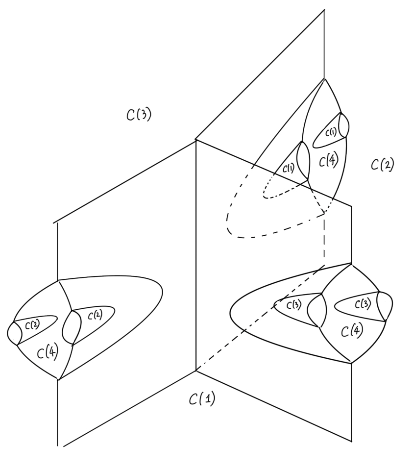
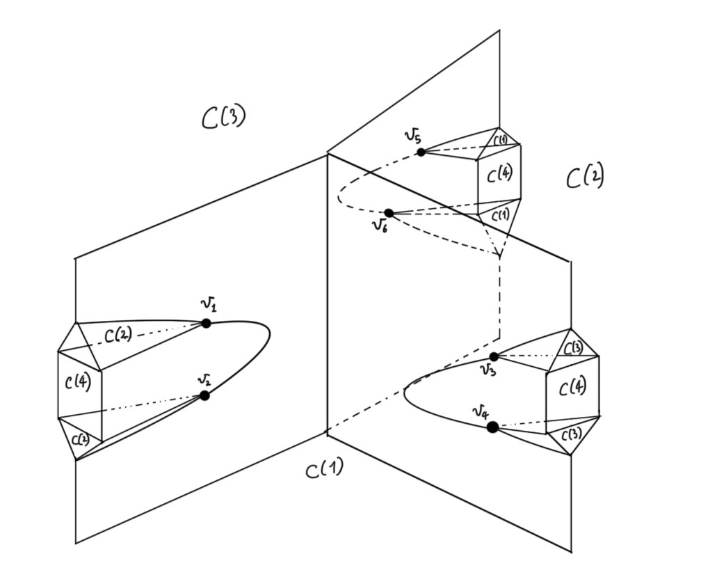
Figure 14: Two configuration types involved in Example 2.

Refer to caption — Figure 15: Left: schematic of the $\mathrm{FVD}(L)$ with 0 vertices. Right: schematic of the $\mathrm{FVD}(L)$ with 6 vertices of Example 2. Each label $C(i)$ denotes a cell in the farthest region of $\ell_{i}$ .

Our classification results yield an algebraically simple method to compute the structure of the Voronoi diagram of four lines. We start by computing the Gaussian map of $\mathrm{FVD}(L)$ [5], which is simple algebraically. We then extract $\mathrm{\Gamma}(\mathrm{FVD}(L))$ by a minor adjustment (concerning the so-called vertices of anomaly of [5]). From $\mathrm{\Gamma}(\mathrm{FVD}(L))$ , we can directly identify the matching base topologies of $\mathrm{NVD}(L)$ and $\mathrm{FVD}(L)$ . Next, we decide if full twists exist by comparing the number of vertices in the base topology with the number of projected trisector intersections. The latter equals the number of real roots of a degree 8 univariate polynomial, which we compute via Sturm’s theorem. If equal, there are no full twists, and the base topology provides the answer; otherwise, we need to locate the full twists. To this end, we derive the real configurations of each bisector (by applying the separation of four branches of a trisector given in [12] to obtain (1) the corresponding simple configurations as in Phase 1, and (2) the number of intersections between all pairs of trisector branches). We compare with the configurations of the base topology, revealing the vertices of full twists, and add them to the base topology via the local modification. All operations can be done in low algebraic degrees, the most expensive being the location of full twists (whose degree is in the range of 8).

In conclusion, we have obtained a complete characterization of Voronoi diagrams of four lines in general position in $\mathbb{R}^{3}$ . This offers a concrete foundation for future research on the Voronoi diagrams of $n$ lines.

References

[1] Pankaj K Agarwal, Boris Aronov, and Micha Sharir. Computing envelopes in four dimensions with applications. In Proceedings of the tenth annual symposium on Computational geometry, pages 348–358, 1994. doi:10.1145/177424.178081.
[2] Boris Aronov. A lower bound on Voronoi diagram complexity. Information Processing Letters, 83(4):183–185, 2002. doi:10.1016/S0020-0190(01)00336-2.
[3] Franz Aurenhammer, Bert Jüttler, and Günter Paulini. Voronoi Diagrams for Parallel Halflines and Line Segments in Space. In Yoshio Okamoto and Takeshi Tokuyama, editors, 28th International Symposium on Algorithms and Computation (ISAAC 2017), volume 92 of Leibniz International Proceedings in Informatics (LIPIcs), pages 7:1–7:10, Dagstuhl, Germany, 2017. Schloss Dagstuhl – Leibniz-Zentrum für Informatik. doi:10.4230/LIPIcs.ISAAC.2017.7.
[4] Franz Aurenhammer, Evanthia Papadopoulou, and Martin Suderland. Piecewise-Linear Farthest-Site Voronoi Diagrams. In Hee-Kap Ahn and Kunihiko Sadakane, editors, 32nd International Symposium on Algorithms and Computation (ISAAC 2021), volume 212 of Leibniz International Proceedings in Informatics (LIPIcs), pages 30:1–30:11, Dagstuhl, Germany, 2021. Schloss Dagstuhl – Leibniz-Zentrum für Informatik. doi:10.4230/LIPIcs.ISAAC.2021.30.
[5] Gill Barequet, Evanthia Papadopoulou, and Martin Suderland. Unbounded regions of high-order Voronoi diagrams of lines and line segments in higher dimensions. Discrete & Computational Geometry, pages 1–29, 2023.
[6] Jean-Daniel Boissonnat, Micha Sharir, Boaz Tagansky, and Mariette Yvinec. Voronoi diagrams in higher dimensions under certain polyhedral distance functions. In Proceedings of the eleventh annual symposium on Computational geometry, pages 79–88, 1995. doi:10.1145/220279.220288.
[7] Bernard Chazelle. An optimal convex hull algorithm and new results on cuttings (extended abstract). In 32nd Annual Symposium on Foundations of Computer Science, San Juan, Puerto Rico, pages 29–38. IEEE Computer Society, 1991. doi:10.1109/SFCS.1991.185345.
[8] L Paul Chew, Klara Kedem, Micha Sharir, Boaz Tagansky, and Emo Welzl. Voronoi diagrams of lines in 3-space under polyhedral convex distance functions. Journal of Algorithms, 29(2):238–255, 1998. doi:10.1006/JAGM.1998.0957.
[9] Tamal K Dey and Wulue Zhao. Approximate medial axis as a Voronoi subcomplex. In Proceedings of the seventh ACM symposium on Solid modeling and applications, pages 356–366, 2002. doi:10.1145/566282.566333.
[10] Herbert Edelsbrunner and Raimund Seidel. Voronoi diagrams and arrangements. Discrete & Computational Geometry, 1:25–44, 1986. doi:10.1007/BF02187681.
[11] Michal Etzion and Ari Rappoport. Computing the Voronoi diagram of a 3-d polyhedron by separate computation of its symbolic and geometric parts. In Proceedings of the fifth ACM symposium on Solid modeling and applications, pages 167–178, 1999. doi:10.1145/304012.304029.
[12] Hazel Everett, Daniel Lazard, Sylvain Lazard, and Mohab Safey El Din. The Voronoi diagram of three lines. Discrete & Computational Geometry, 42(1):94–130, 2009. doi:10.1007/S00454-009-9173-3.
[13] Marc Glisse. Lower bound on the Voronoi diagram of lines in $\mathbb{R}^{d}$ , 2021. arXiv:2103.17251.
[14] Michael Hemmer, Ophir Setter, and Dan Halperin. Constructing the exact Voronoi diagram of arbitrary lines in three-dimensional space: with fast point-location. In European Symposium on Algorithms, pages 398–409. Springer, 2010. doi:10.1007/978-3-642-15775-2_34.
[15] Christian Icking and Lihong Ha. A tight bound for the complexity of Voroni diagrams under polyhedral convex distance functions in 3d. In Proceedings of the thirty-third annual ACM symposium on Theory of computing, pages 316–321, 2001.
[16] Victor Klee. On the complexity of d-dimensional Voronoi diagrams. Archiv der Mathematik, 34(1):75–80, 1980.
[17] Vladlen Koltun and Micha Sharir. Polyhedral Voronoi diagrams of polyhedra in three dimensions. In Proceedings of the eighteenth annual symposium on Computational geometry, pages 227–236, 2002. doi:10.1145/513400.513428.
[18] Vladlen Koltun and Micha Sharir. Three dimensional Euclidean Voronoi diagrams of lines with a fixed number of orientations. In Proceedings of the eighteenth annual symposium on Computational geometry, pages 217–226, 2002. doi:10.1145/513400.513427.
[19] Joseph S. B. Mitchell and Joseph O’Rourke. Computational geometry column 42. International Journal of Computational Geometry & Applications, 11(5):573–582, 2001. doi:10.1142/S0218195901000651.
[20] Raimund Seidel. On the number of faces in higher-dimensional Voronoi diagrams. In Proceedings of the third annual symposium on Computational geometry, pages 181–185, 1987. doi:10.1145/41958.41977.
[21] Micha Sharir. Almost tight upper bounds for lower envelopes in higher dimensions. Discrete & Computational Geometry, 12:327–345, 1994. doi:10.1007/BF02574384.
[22] Zeyu Wang. Search engine for the Voronoi diagram of four lines in $\mathbb{R}^{3}$ , March 2026. doi:10.5281/zenodo.19090548.

[bib.bib1] [1] Pankaj K Agarwal, Boris Aronov, and Micha Sharir. Computing envelopes in four dimensions with applications. In Proceedings of the tenth annual symposium on Computational geometry, pages 348–358, 1994. doi:10.1145/177424.178081.

[bib.bib2] [2] Boris Aronov. A lower bound on Voronoi diagram complexity. Information Processing Letters, 83(4):183–185, 2002. doi:10.1016/S0020-0190(01)00336-2.

[bib.bib3] [3] Franz Aurenhammer, Bert Jüttler, and Günter Paulini. Voronoi Diagrams for Parallel Halflines and Line Segments in Space. In Yoshio Okamoto and Takeshi Tokuyama, editors, 28th International Symposium on Algorithms and Computation (ISAAC 2017), volume 92 of Leibniz International Proceedings in Informatics (LIPIcs), pages 7:1–7:10, Dagstuhl, Germany, 2017. Schloss Dagstuhl – Leibniz-Zentrum für Informatik. doi:10.4230/LIPIcs.ISAAC.2017.7.

[bib.bib4] [4] Franz Aurenhammer, Evanthia Papadopoulou, and Martin Suderland. Piecewise-Linear Farthest-Site Voronoi Diagrams. In Hee-Kap Ahn and Kunihiko Sadakane, editors, 32nd International Symposium on Algorithms and Computation (ISAAC 2021), volume 212 of Leibniz International Proceedings in Informatics (LIPIcs), pages 30:1–30:11, Dagstuhl, Germany, 2021. Schloss Dagstuhl – Leibniz-Zentrum für Informatik. doi:10.4230/LIPIcs.ISAAC.2021.30.

[bib.bib5] [5] Gill Barequet, Evanthia Papadopoulou, and Martin Suderland. Unbounded regions of high-order Voronoi diagrams of lines and line segments in higher dimensions. Discrete & Computational Geometry, pages 1–29, 2023.

[bib.bib6] [6] Jean-Daniel Boissonnat, Micha Sharir, Boaz Tagansky, and Mariette Yvinec. Voronoi diagrams in higher dimensions under certain polyhedral distance functions. In Proceedings of the eleventh annual symposium on Computational geometry, pages 79–88, 1995. doi:10.1145/220279.220288.

[bib.bib7] [7] Bernard Chazelle. An optimal convex hull algorithm and new results on cuttings (extended abstract). In 32nd Annual Symposium on Foundations of Computer Science, San Juan, Puerto Rico, pages 29–38. IEEE Computer Society, 1991. doi:10.1109/SFCS.1991.185345.

[bib.bib8] [8] L Paul Chew, Klara Kedem, Micha Sharir, Boaz Tagansky, and Emo Welzl. Voronoi diagrams of lines in 3-space under polyhedral convex distance functions. Journal of Algorithms, 29(2):238–255, 1998. doi:10.1006/JAGM.1998.0957.

[bib.bib9] [9] Tamal K Dey and Wulue Zhao. Approximate medial axis as a Voronoi subcomplex. In Proceedings of the seventh ACM symposium on Solid modeling and applications, pages 356–366, 2002. doi:10.1145/566282.566333.

[bib.bib10] [10] Herbert Edelsbrunner and Raimund Seidel. Voronoi diagrams and arrangements. Discrete & Computational Geometry, 1:25–44, 1986. doi:10.1007/BF02187681.

[bib.bib11] [11] Michal Etzion and Ari Rappoport. Computing the Voronoi diagram of a 3-d polyhedron by separate computation of its symbolic and geometric parts. In Proceedings of the fifth ACM symposium on Solid modeling and applications, pages 167–178, 1999. doi:10.1145/304012.304029.

[bib.bib12] [12] Hazel Everett, Daniel Lazard, Sylvain Lazard, and Mohab Safey El Din. The Voronoi diagram of three lines. Discrete & Computational Geometry, 42(1):94–130, 2009. doi:10.1007/S00454-009-9173-3.

[bib.bib13] [13] Marc Glisse. Lower bound on the Voronoi diagram of lines in $\mathbb{R}^{d}$ , 2021. arXiv:2103.17251.

[bib.bib14] [14] Michael Hemmer, Ophir Setter, and Dan Halperin. Constructing the exact Voronoi diagram of arbitrary lines in three-dimensional space: with fast point-location. In European Symposium on Algorithms, pages 398–409. Springer, 2010. doi:10.1007/978-3-642-15775-2_34.

[bib.bib15] [15] Christian Icking and Lihong Ha. A tight bound for the complexity of Voroni diagrams under polyhedral convex distance functions in 3d. In Proceedings of the thirty-third annual ACM symposium on Theory of computing, pages 316–321, 2001.

[bib.bib16] [16] Victor Klee. On the complexity of d-dimensional Voronoi diagrams. Archiv der Mathematik, 34(1):75–80, 1980.

[bib.bib17] [17] Vladlen Koltun and Micha Sharir. Polyhedral Voronoi diagrams of polyhedra in three dimensions. In Proceedings of the eighteenth annual symposium on Computational geometry, pages 227–236, 2002. doi:10.1145/513400.513428.

[bib.bib18] [18] Vladlen Koltun and Micha Sharir. Three dimensional Euclidean Voronoi diagrams of lines with a fixed number of orientations. In Proceedings of the eighteenth annual symposium on Computational geometry, pages 217–226, 2002. doi:10.1145/513400.513427.

[bib.bib19] [19] Joseph S. B. Mitchell and Joseph O’Rourke. Computational geometry column 42. International Journal of Computational Geometry & Applications, 11(5):573–582, 2001. doi:10.1142/S0218195901000651.

[bib.bib20] [20] Raimund Seidel. On the number of faces in higher-dimensional Voronoi diagrams. In Proceedings of the third annual symposium on Computational geometry, pages 181–185, 1987. doi:10.1145/41958.41977.

[bib.bib21] [21] Micha Sharir. Almost tight upper bounds for lower envelopes in higher dimensions. Discrete & Computational Geometry, 12:327–345, 1994. doi:10.1007/BF02574384.

[bib.bib22] [22] Zeyu Wang. Search engine for the Voronoi diagram of four lines in $\mathbb{R}^{3}$ , March 2026. doi:10.5281/zenodo.19090548.

The Voronoi Diagram of Four Lines in ℝ𝟑

Abstract

Keywords and phrases:

Copyright and License:

2012 ACM Subject Classification:

Related Version:

Supplementary Material:

Acknowledgements:

Funding:

DOI:

Event:

Editors:

Series and Publisher:

1 Introduction

Contribution.

Theorem 1.

Theorem 2.

2 Preliminaries

Lemma 3.

2.1 Algebraic framework and geometric reinterpretation

Lemma 4 ([12]).

3 Some combinatorial results on Voronoi diagrams of lines in ℝ𝟑

Lemma 5.

Lemma 6.

Lemma 7.

Lemma 8.

Theorem 9.

4 Twists

Definition 10.

Definition 11.

Lemma 12.

4.1 Full twists

Lemma 13.

Proof sketch.

Local modification.

4.2 Partial twists and further properties

Lemma 14.

Proof.

Corollary 15.

Proof sketch of Lemma 12.

Lemma 16.

Proof sketch.

5 Identifying the Voronoi topologies by exhaustive search

5.1 Properties of configurations

Lemma 17.

Proof sketch.

Corollary 18.

Lemma 19.

Proof sketch.

Lemma 20.

5.2 A search algorithm, proving Theorems 1 and 2

Observation 21.

Proof sketch of Theorem 1.

Proof sketch of Theorem 2.

6 Examples and concluding remarks

Example 1: Voronoi diagram of four lines with 0 vertices.

Example 2: Voronoi diagram of four lines with 6 vertices.

References

The Voronoi Diagram of Four Lines in $\mathbb{R}^{3}$

3 Some combinatorial results on Voronoi diagrams of lines in $\mathbb{R}^{3}$