Simplicial Approximation to CW Complexes with Spherical Delaunay Triangulations

Tinarrage, Raphaël

doi:10.4230/LIPIcs.SoCG.2026.93

Simplicial Approximation to CW Complexes with Spherical Delaunay Triangulations

Raphaël Tinarrage

Institute of Science and Technology Austria, Klosterneuburg, Austria

Abstract

Simplicial approximation provides a framework for constructing simplicial complexes that are homotopy equivalent to a given manifold, provided a CW structure is explicitly known. However, its conventional implementation quickly becomes intractable on a computer: barycentric subdivision produces poorly shaped simplices, and the star condition introduces many vertices. To address these limitations, this article develops a subdivision scheme based on spherical Delaunay triangulations, which attains better refinement properties than barycentric subdivisions. Moreover, the star condition is reframed as two independent problems, one geometric and the other combinatorial, respectively tackled in the language of locally equiconnected spaces and the list homomorphism problem, allowing an exponential reduction in the number of vertices. Via a prototype implementation, we obtain simplicial complexes homotopy equivalent to Grassmannians and Stiefel manifolds up to dimension 5.

Keywords and phrases:

Triangulation of manifolds, Simplicial approximation, CW complexes, Delaunay complexes, List homomorphism problem, Topological Data Analysis

Copyright and License:

2012 ACM Subject Classification:

Mathematics of computing

\rightarrow

Mesh generation ; Mathematics of computing

\rightarrow

Combinatoric problems ; Mathematics of computing

\rightarrow

Algebraic topology ; Mathematics of computing

\rightarrow

Mathematical software performance

Editors:

Hee-Kap Ahn, Michael Hoffmann, and Amir Nayyeri

Series and Publisher:

Leibniz International Proceedings in Informatics, Schloss Dagstuhl – Leibniz-Zentrum für Informatik

1 Introduction

1.1 Topology software

In computational topology, a popular way to represent a topological space is via a simplicial complex. Once a space is triangulated, it can be explored algorithmically, and a range of homotopy invariants can be evaluated [36, 37, 38, 69, 39, 64, 65, 66, 112, 90]. More generally, triangulations open the door to many further developments: they allow us to test conjectures and discover new properties [16, 15], they serve as a benchmark for comparing software [14, 9, 108] and they lay the foundation for new data analysis techniques [103, 106, 59, 111].

Over the past two decades, software for computations on simplicial complexes has advanced substantially. Existing libraries span a wide range of goals, from algebra to geometry and data analysis. They have underpinned numerous concrete advances: proofs and counterexamples in 3-manifold topology with Regina and SnapPy [35, 48]; large-scale enumerations that tested conjectures with BISTELLAR and Twister [18, 13]; new homotopy and cohomology computations in Kenzo and HAP [50, 56]; and persistent homology pipelines that surfaced new properties of datasets with GUDHI, Ripser, and TTK [91, 11, 110], among many others.

On the other hand, computational topology lacks explicit examples of triangulated manifolds, as noted in [16, 66, 9, 108]. By explicit, we mean stored on a computer as a list of simplices, or obtainable in reasonable time by an implemented algorithm. This is especially striking in dimension 4 and above, as summarized in Table 1, which collects known triangulations of certain classical manifolds. Apart from the real and complex projective spaces, most triangulations are “accidental”, i.e., arising from special homeomorphisms with known spaces. The aim of this article is to develop an algorithm for triangulating new spaces.

Table 1: Known explicit triangulations of a selection of manifolds.

Space	Known cases	References / Known identifications
Real projective space $\mathbb{R}P^{n}$	$n\geq 1$	[83, 8, 4]
Complex projective space $\mathbb{C}P^{n}$	$n\geq 1$	[84, 102, 6, 7, 101, 49]
Special orthogonal group $\mathrm{SO}(n)$	$n\leq 4$	$\mathrm{SO}(3)\cong\mathbb{R}P^{3}$ , $\mathrm{SO}(4)\cong S^{3}\times\mathrm{SO}(3)$
Special unitary group $\mathrm{SU}(n)$	$n\leq 2$	$\mathrm{SU}(2)\cong S^{3}$
Unitary group $\mathrm{U}(n)$	$n=1$	$\mathrm{U}(1)\cong S^{1}$
Real Stiefel manifold $\mathcal{V}(d,n)$	$d=1$ or $n\leq 4$	$\mathcal{V}(1,n)\cong S^{n-1}$ , $\mathcal{V}(d-1,d)\cong\mathrm{SO}(d)$
Real Grassmannian $\mathcal{G}(d,n)$	$d=1$ or $d=n-1$	$\mathcal{G}(1,n)\cong\mathcal{G}(n-1,n)\cong\mathbb{R}P^{n-1}$

1.2 Related work

Traditionally, explicit triangulations of manifolds are obtained by two main approaches. The first is combinatorial and relies on specific descriptions of the manifolds under consideration. For example, small triangulations of $\mathbb{R}P^{n}$ have recently been constructed by exploiting its realization from a symmetric polytope [4]. Topological properties can also guide the enumeration of combinatorial manifolds, as in the work of Lutz [87, 107]. However, combinatorial complexity grows rapidly with the dimension. Thus, in dimensions 3 and 4, more structured constructions are preferred, based on layered triangulations [76, 75, 77], Dehn fillings [52], Heegaard diagrams [57, 74, 58], and Kirby diagrams [33, 34]. The present work follows this perspective by exploiting the CW structure of the spaces involved, which is well understood.

Sampling-based methods offer a different viewpoint. A large body of work studies how to reconstruct an embedded manifold $\mathcal{M}\subset\mathbb{R}^{n}$ from a finite sample $X\subset\mathbb{R}^{n}$ . The goal is usually not to recover a triangulation of $\mathcal{M}$ itself, but rather a simplicial complex with the same homotopy type. A standard construction is the Čech complex. Recovery is guaranteed when the sampling density is sufficiently fine relative to an appropriate condition number, typically the reach of $\mathcal{M}$ [94]. Quantitative refinements use less restrictive geometric quantities, such as the $\mu$ -reach [40, 78], weak feature size [41], local feature size [42], convexity defects [5], and convexity radius [61]. In higher dimensions, however, the Čech complex may be prohibitively expensive to compute, and one may instead use the Vietoris–Rips complex, which depends only on pairwise distances. Following the foundational results of Hausmann and Latschev [73, 85], quantitative guarantees have been established in terms of the reach [88, 89], the $\mu$ -reach [78], and convexity defects [5]. Other approaches rely on Delaunay complexes [23, 24, 22, 1], witness complexes [104, 70, 25, 26], and metric thickenings [2, 3].

These methods nevertheless remain computationally demanding. Vietoris–Rips complexes are the cheapest to compute, but their guarantees are weaker and they typically require many vertices. Čech complexes present the same difficulty, as they may contain a large number of simplices, potentially of high dimension. In contrast, more refined constructions such as Delaunay complexes require substantial computation time and scale poorly with dimension.

Grassmannians $\mathcal{G}(d,n)$ are a notable example, regarded as difficult to triangulate. Theoretical results indicate that the minimal number of facets increases exponentially with $n$ [68]. Knudson considered triangulating $\mathcal{G}(2,4)$ by embedding it into $\mathbb{R}^{16}$ and constructing a Vietoris–Rips complex [79]. In practice, the approach amounted to increasing the scale until obtaining a complex with the expected homology. This proved too costly in memory, and a witness complex was used instead. Although a complex with the correct homology was found, this construction does not satisfy the hypotheses of the available theorems.

1.3 Contributions

In Algorithm 2 we present an implementation of simplicial approximation to CW complexes, a framework well established in theory yet overlooked in practice. Given a CW structure on a topological space, the algorithm outputs a homotopy equivalent simplicial complex. Although not homeomorphic, such a complex still suffices for many of the applications mentioned above. Crucially, our complexes are equipped with a point location routine, making them practical surrogates for the manifold in data-driven applications.

Turning the textbook construction into a practical implementation requires several adjustments; in particular, we aim to keep the resulting complexes as small as possible. To this end, in Section 2, we adopt Delaunay refinement instead of barycentric subdivision; in Section 3, we build a simplicial mapping cone that avoids subdividing the complex; and in Section 4, we substitute the star condition for a more efficient constraint satisfaction problem.

We implemented two versions of the algorithm, using either global or local refinement. Only the first is currently proven to terminate, but the second often produces smaller complexes. In both cases, when the algorithm terminates, the output is correct (see Theorem 13).

The software is provided as supplementary material.¹¹1Fully implemented prototype in Python: https://github.com/raphaeltinarrage/cw2simp The repository includes complexes homotopy equivalent to $\mathcal{G}(2,4)$ and $\mathcal{V}(2,4)$ (of dimensions $4$ and $5$ ), which were not available prior to this work. We intend to address higher-dimensional examples in future work by increasing computational resources; the current results were obtained on a personal laptop.

The algorithm is sketched in the next section. In Sections 2, 3, and 4 we develop the theoretical results required for its implementation. Proofs appear in the full version of the article.

1.4 Overview and discussion of the construction

CW complexes.

The theoretical background can be found in Hatcher’s book [72, Section 2.C]. A CW complex of dimension $n$ is a topological space $X$ endowed with a decomposition $X=X^{n}\supset X^{n-1}\supset\cdots\supset X^{0}$ where $X^{0}$ is finite and each $X^{d}$ is equal to a disjoint union

X^{d}=X^{d-1}\coprod_{1\leq i\leq m(d)}e_{i}^{d},

where each $e_{i}^{d}$ , called a $d$ -cell, is homeomorphic to an open ball of dimension $d$ , and $m(d)$ is their number. It is required that the homeomorphism extends to the closed ball $B^{d}$ , yielding a map $\Phi_{i}^{d}\colon B^{d}\to\bar{e}_{i}^{d}\subset X^{d}$ , called the characteristic map. Its restriction to the boundary of $B^{d}$ – i.e., the sphere $S^{d-1}$ – is called the gluing map and is denoted $\phi_{i}^{d}\colon S^{d-1}\to X^{d-1}$ . In other words, $X^{d}$ is homeomorphic to the gluing of $d$ -balls along their boundary on $X^{d-1}$ :

X^{d}\cong X^{d-1}\cup_{\phi_{1}^{d}}B^{d}\cup_{\phi_{2}^{d}}B^{d}\cup\dots% \cup_{\phi_{m(d)}^{d}}B^{d}.

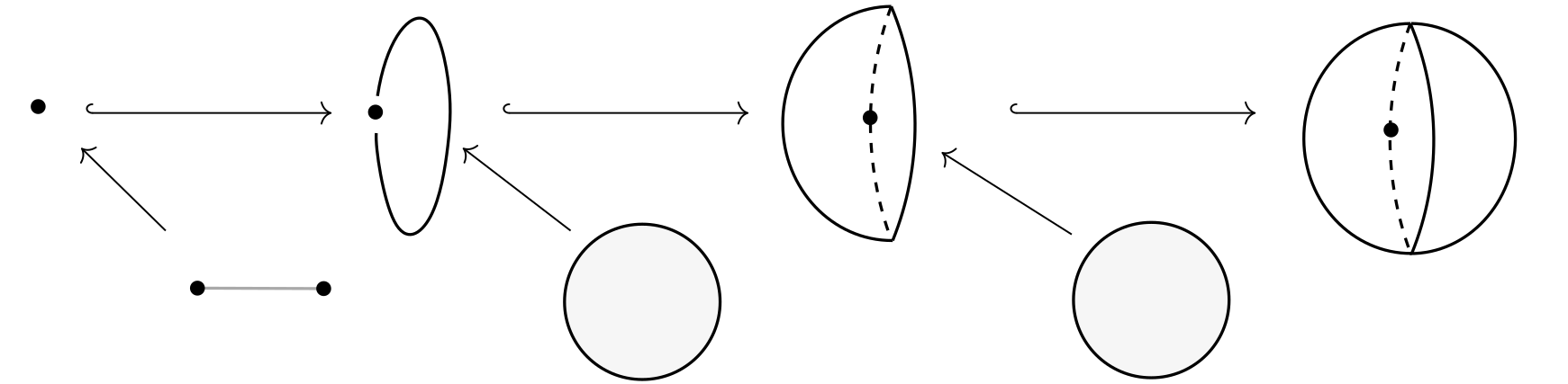
Figure 1(a) shows a CW structure on $S^{2}$ , made of one $0$ - and $1$ -cell and two $2$ -cells. Figure 1(b) depicts the usual structure on $\mathbb{R}P^{2}$ : one cell per dimension and a gluing map $\phi^{2}\colon S^{1}\to S^{1}$ of degree 2. Similarly, all the manifolds in Table 1 admit a well-known CW structure. We refer the interested reader to [92, Section 6] for the classical structure on Grassmannians, [72, Section 3.D] for Stiefel manifolds and orthogonal groups, and [113] for unitary groups.

(a)

S^{2}

.

(b)

\mathbb{R}P^{2}

.

Figure 1: Examples of CW structures on the sphere

S^{2}

(four cells in total) and the projective plane

\mathbb{R}P^{2}

(one cell per dimension). If only one

d

-cell is attached, we omit the subscript in

e_{i}^{d}

.

Sketch of the approach.

One can “convert” a CW complex into a simplicial complex by gluing simplicial balls instead of cells; the idea is sketched in Figure 2. The construction proceeds inductively on the dimension. Suppose we have already built a simplicial complex $L^{d}$ homotopy equivalent to the $d$ -skeleton $X^{d}$ ; we denote by $|L^{d}|$ its geometric realization. For each $(d+1)$ -cell $e^{d+1}_{i}$ , we perform the following steps:

$\blacksquare$

We apply simplicial approximation (see below) to the gluing map $\phi_{i}^{d+1}\colon S^{d}\to|L^{d}|$ . This yields a triangulation $K_{i}^{d}$ of $S^{d}$ and a simplicial map $g^{d+1}_{i}\colon K^{d}_{i}\to L^{d}$ homotopic to $\phi_{i}^{d+1}$ .
$\blacksquare$

From $K^{d}_{i}$ , we construct a simplicial ball $B(K^{d}_{i})$ with boundary $K^{d}_{i}$ and glue it to $L^{d}$ along this boundary via $g^{d+1}_{i}$ . This amounts to the simplicial mapping cone of $g^{d+1}_{i}$ .

After all $(d+1)$ -cells have been attached, the resulting complex $L^{d+1}$ is homotopy equivalent to the skeleton $X^{d+1}$ , and the procedure can be iterated in the next dimension.

Refer to caption — (a) Diagram induced by the CW structure on $S^{2}$ in Figure 1(a).

Computational obstacles.

Conventionally, the simplicial approximation of $\phi_{i}^{d+1}\colon S^{d}\to|L^{d}|$ is obtained as follows: one starts from any triangulation $K$ of $S^{d}$ and repeatedly applies barycentric subdivision until the triangulation is fine enough. More precisely, one stops when the map satisfies the star condition: each closed star of a vertex $v\in K$ is mapped by $\phi_{i}^{d+1}$ into the open star of some vertex $w\in L^{d}$ . The simplicial approximation theorem ensures that this procedure terminates [72, Theorem 2C.1]. The assignment of vertices $v\mapsto w$ defines a simplicial map $g^{d+1}_{i}$ homotopic to $\phi_{i}^{d+1}$ (through a homotopy that is linear on each simplex).

In practice, this approach quickly becomes intractable for two reasons. First, barycentric subdivision introduces a large number of vertices: a $d$ -simplex is converted into a complex with $2^{d+1}-1$ vertices. In Section 2, we propose to use instead the Delaunay complexes and their refinements. We show in Theorem 4 that Delaunay refinement enjoys better approximation properties than barycentric subdivision: the simplices shrink more rapidly.

Secondly, the star condition itself is too coarse: each facet of $L^{d}$ requires $d+1$ vertices of $K$ that are mapped into it. This contributes further to the exponential growth in the number of vertices. In Section 4, we avoid the star condition altogether by decomposing the problem into two parts: a geometric step (constructing a homotopy equivalence) and a combinatorial step (constructing a simplicial map). Proposition 12 ensures that this procedure is correct.

Last, the standard construction of a simplicial mapping cone, going back to Cohen [47], relies on the barycentric subdivision of $K$ , which again leads to large complexes. In Section 3, we consider a lighter triangulation, based on staircase triangulation of products. Proposition 7 shows that this object is homotopy equivalent to the standard mapping cone.

2 Successive refinements of spherical Delaunay triangulations

Our construction begins with a refinement scheme for spherical Delaunay complexes, which generates arbitrarily fine triangulations and is well suited to concrete implementation.

2.1 Spherical Delaunay triangulations

Definition

Let $X\subset\mathbb{R}^{d}$ be finite. A subset of $d+1$ points has the empty circle property if its circumscribing (open) ball is empty of points of $X$ . These subsets form the facets of an abstract simplicial complex $\mathrm{Del}(X)$ , called the Delaunay complex. Under the genericity assumption that no subset of $d+2$ points lies on the same sphere, $\mathrm{Del}(X)$ is naturally embedded in $\mathbb{R}^{d}$ [20].

These definitions adapt to the spherical case: given a subset $X$ of the unit sphere $S^{d}\subset\mathbb{R}^{d+1}$ , the empty circle property is understood with respect to the geodesic distance on $S^{d}$ ; the resulting complex is called the spherical Delaunay complex and is still denoted $\mathrm{Del}(X)$ . If no subset of $d+2$ points lies on the same geodesic sphere, then it is naturally embedded in $\mathbb{R}^{d+1}$ . We shall implicitly make this assumption throughout the article.

It is well-known that the spherical Delaunay complex coincides with the boundary of the convex hull of its vertices, thus reducing the computation of $\mathrm{Del}(X)$ to $\mathrm{conv}(X)$ [31]. In our implementation, we used Qhull, a popular software package for computing convex hulls [10].

Point location

A natural map $|\mathrm{Del}(X)|\to S^{d}$ is given by the scaling $x\mapsto x/\|x\|$ , which is a homeomorphism provided that the origin is included in the interior of the convex hull of $X$ . A set $X$ satisfying this assumption will be referred to as admissible, and $\mathrm{Del}(X)$ as an admissible triangulation. We call the inverse homeomorphism $r\colon S^{d}\to|\mathrm{Del}(X)|$ the radial projection. Computationally speaking, the radial projection of $x\in S^{d}$ is found by identifying a facet $\sigma\in\mathrm{Del}(X)$ to which $r(x)$ belongs, then computing a simple line/hyperplane intersection.

We perform point location via a conventional Jump-and-Walk strategy [93]: it consists of choosing a first candidate $\sigma\in\mathrm{Del}(X)$ , hopefully close to $r(x)$ , then walking through its neighbor facets until reaching one that contains $r(x)$ . Unlike popular software packages such as STRIPACK or CGAL [109, 98], our implementation does not make use of spherical geometric predicates. Instead, we project $\mathrm{Del}(X)$ into the tangent space of $S^{d}$ at $x$ via the stereographic projection $p\colon S^{d}\setminus\{-x\}\to T_{x}S^{d}$ and work in the induced Euclidean triangulation (the simplices are replaced with the convex hull of their vertices). This approach lets us reuse Euclidean routines already present in our code. In this step, we exclude from $\mathrm{Del}(X)$ all simplices incident to $-x$ , since their images under $p$ are not defined.

A caveat is that stereographic projection distorts geodesics: in general, the image geodesic simplex $p(|\sigma|)$ need not coincide with the linear simplex $\mathrm{conv}(\{p(v_{0}),\dots,p(v_{d})\})$ on the image of its vertices. Consequently, a point might map to the “wrong” linear simplex. The next lemma shows that this cannot happen at the pole $x$ , which justifies our procedure.

Lemma 1.

Let $\sigma=[v_{0},\dots,v_{d}]\in\mathrm{Del}(X)$ and $x\in S^{d}$ such that $r(x)\in|\sigma|$ . Then $p(x)\in\mathrm{conv}(\{p(v_{0}),\dots,p(v_{d})\})$ , where $p$ is the stereographic projection at $x$ .

2.2 Global Delaunay refinements

Given a spherical Delaunay triangulation $\mathrm{Del}(X_{0})$ with vertex set $X_{0}\subset S^{d}$ , one obtains a finer triangulation by choosing additional points $Y_{0}\subset S^{d}$ and building the Delaunay complex on $X_{1}=X_{0}\cup Y_{0}$ . The new points are called Steiner points, and this procedure is known as a Delaunay refinement. This construction can be iterated, yielding a sequence of Steiner points $Y_{0}$ , $Y_{1}$ , $Y_{2}$ , $\dots$ and complexes $\mathrm{Del}(X_{0})$ , $\mathrm{Del}(X_{1})$ , $\mathrm{Del}(X_{2})$ , $\dots$

In computational geometry, Delaunay refinement lies at the core of popular algorithms for generating and refining Euclidean meshes; see [43] for a modern presentation. For instance, Chew’s and Ruppert’s algorithms [44, 45, 99] take a set of input constraints (e.g., boundary segments that must appear as edges) and iteratively improve the mesh by eliminating poor-quality triangles. The refinement step consists of marking a bad triangle and inserting its circumcenter as a new vertex, after which the Delaunay triangulation is recomputed.

Our objective here is different: we seek triangulations whose simplices can be made arbitrarily small, enabling the simplicial approximation of maps described in Section 1.4. To this end, we introduce several families of Delaunay-based refinements, visualized in Figure 3.

Barycentric refinement:: Inspired by barycentric subdivision, we let the Steiner points $Y_{i}$ be the barycenters of all simplices of $\mathrm{Del}(X_{i})$ , except its vertices.
Edgewise refinement:: We may instead insert the midpoints of all edges of $\mathrm{Del}(X_{i})$ , in analogy with the popular Coxeter-Freudenthal-Kuhn subdivisions of simplices, also called edgewise subdivisions [17, 54, 67, 97, 82, 80, 46, 27, 32, 19, 28, 29].
Minicenter refinement:: Closer in spirit to conventional Delaunay refinement, we also consider inserting the minicenters of the facets (centers of minimal enclosing balls). We favor minicenters over circumcenters because, unlike circumcenters, they always lie inside the simplex that defines them, which better reflects the local nature of classical subdivision.
Centroid refinement:: Finally, we may insert the barycenters of only the facets of $\mathrm{Del}(X_{i})$ (the maximal simplices), standing as a cheaper alternative to barycentric refinement.

In all cases, the spherical Steiner points are considered (i.e., spherical barycenters or minicenters). This is equivalent to computing their Euclidean counterpart in the ambient space $\mathbb{R}^{d+1}$ and projecting them onto the sphere; see, for instance, Fiedler’s book [63, Section 5.4].

(a) Local picture: A Delaunay complex on a set of four points in

\mathbb{R}^{2}

and the four refinements proposed.

Initial complex

Barycentric

Edgewise

Minicenter

Centroid

(b) Global picture: Spherical Delaunay complexes after three or four refinements of an initial triangulation of

S^{2}

(the boundary of the standard simplex). The colors indicate the simplex ratio inradius/circumradius.

Figure 3: We employ Delaunay refinement as a subdivision scheme for triangulations of

S^{d}

.

Note that, strictly speaking, $\mathrm{Del}(X_{i+1})$ is not a subdivision of $\mathrm{Del}(X_{i})$ : when realized on the sphere, a simplex of $\mathrm{Del}(X_{i+1})$ need not be contained in a single simplex of $\mathrm{Del}(X_{i})$ . This can be seen in Figure 3(a), where only the edgewise and minicenter refinements are subdivisions. As a consequence, it is not immediate that simplices become smaller under refinement. In particular, adding a point to a Delaunay triangulation can increase the maximal edge length, as illustrated in Figure 4 (shown in the plane for clarity). Instead, we show that the maximal (spherical) circumradius of $\mathrm{Del}(X_{i})$ , denoted $\rho_{\mathrm{circ}}(\mathrm{Del}(X_{i}))$ , decreases monotonically to zero. Since the maximal diameter of the simplices of $\mathrm{Del}(X_{i})$ is at most twice its maximal circumradius, it follows that the maximal diameter also tends to zero.

Figure 4: Adding a point to a Delaunay complex may increase the maximal edge length.

A convenient quantity to study a Delaunay complex on a subset $X\subset S^{d}$ is its covering radius (also known as sampling radius) [21, 20]. On the sphere, it is defined by

\rho_{\mathrm{cov}}(X)=\sup_{y\in S^{d}}\inf_{x\in X\vphantom{S^{d}}}\mathrm{d% }(x,y),

where $\mathrm{d}(x,y)$ is the geodesic (great-circle) distance on the sphere. We note that the set $X$ is admissible as long as $\rho_{\mathrm{cov}}(X)<\pi/2$ (i.e., $X$ is not contained in a closed hemisphere).

The maximal circumradius and covering radius are related by the following standard result.

Lemma 2.

For every admissible finite subset $X\subset S^{d}$ , it holds that $\rho_{\mathrm{circ}}(\mathrm{Del}(X))=\rho_{\mathrm{cov}}(X)$ .

We take advantage of this shift to the covering radius to prove the following lemma.

Lemma 3.

Consider a finite subset $X\subset S^{d}$ and let $Y$ denote the Steiner points associated with $\mathrm{Del}(X)$ . Assume that $\rho_{\mathrm{cov}}(X)\leq\pi/3$ . Then

\rho_{\mathrm{cov}}(X\cup Y)\leq\alpha\rho_{\mathrm{cov}}(X),

where $\alpha=\alpha^{\prime}/\cos(\rho_{\mathrm{cov}}(X))$ , and $\alpha^{\prime}$ depends on the chosen refinement, as given in the table

Refinement	Edgewise	Minicenter	Centroid
$\alpha^{\prime}$	$1/\sqrt{2}$	$1/\sqrt{2}$	$d/(d+1)$

The quantity $\cos(\rho_{\mathrm{cov}}(X))$ reflects the spherical distortion of lengths; it goes to 1 as the covering radius goes to zero. A similar lemma can be obtained in the Euclidean case, without this factor. We point out that we have not been able to obtain a satisfactory bound for barycentric refinement; for lack of a better estimate, we use the bound for edgewise refinement.

By iterating this lemma, we obtain our main result on Delaunay refinement.

Theorem 4.

Assume the initial sample $X_{0}\subset S^{d}$ is sufficiently dense so that $\alpha<1$ , where $\alpha=\alpha(X_{0})$ is defined in Lemma 3. Then the $n^{\mathrm{th}}$ iteration of Delaunay refinement satisfies

\rho_{\mathrm{cov}}(X_{n})\leq\alpha^{n}\rho_{\mathrm{cov}}(X_{0}).

In particular, the maximal diameter of simplices of $\mathrm{Del}(X_{n})$ goes to zero.

$\blacktriangleright$ Remark 5.

This result highlights a notable distinction between Delaunay refinement and standard subdivision. While barycentric refinement reduces diameters asymptotically by $1/\sqrt{2}$ (at most), the best bound for barycentric subdivision is $d/(d+1)$ . Likewise, centroid refinement reduces them by $d/(d+1)$ , even though it introduces only one vertex per facet.

3 Simplicial mapping cones with staircase triangulations

In this section, we assume that a simplicial approximation $g\colon K\to L$ of $f\colon S^{d}\to|L|$ is given. We build a simplicial mapping cone $C_{\mathrm{simp}}(g)$ and show it is homotopy equivalent to the usual mapping cone $C(f)$ . The construction proceeds by building a simplicial ball $B(K)$ through staircase triangulation, which we first recall. Although this construction already appears in the literature, notably in [105, Exercise E, p. 151] and [12, Proposition 2], we include a detailed account here in order to collect the properties that will be used in the sequel.

3.1 Triangulation of the ball

Staircase triangulation of the prism

To triangulate the Cartesian product of a $d$ -simplex $\sigma$ with an interval $I=[0,1]$ , the staircase triangulation consists of first ordering the vertices $\{v_{0},\dots,v_{d}\}$ of $\sigma$ , taking a copy $\{v_{0}^{\prime},\dots,v_{d}^{\prime}\}$ , and inserting the simplices $\sigma_{k}=[v_{k},\dots,v_{d},v_{0}^{\prime},\dots,v_{k}^{\prime}]$ for all $k\in\{0,\dots,d\}$ [86]. We shall refer to the product $|\sigma|\times I$ as a prism, and its face $[v_{k},\dots,v_{d}]$ (resp. $[v_{0}^{\prime},\dots,v_{k}^{\prime}]$ ) as the inner face (resp. the outer face). Geometrically, they correspond to $|\sigma|\times\{0\}$ and $|\sigma|\times\{1\}\subset|\sigma|\times I$ .

The relation $\sigma_{k}<\sigma_{k+1}$ defines an order on the prism’s $d+1$ facets. In particular, the following observation will be useful later: vertical straight lines in the prism – i.e., of the form $t\mapsto(x,t)$ for a certain $x\in|\sigma|$ – cross each facet consecutively. Indeed, for $k\in\{1,\dots,d-1\}$ , the only neighboring facets of $\sigma_{k}$ are $\sigma_{k-1}$ and $\sigma_{k+1}$ ; see Figures 5(a) and 5(b). On the other hand, horizontal sections of the prism – i.e., sets $|\sigma|\times\{t\}$ for $t\in[0,1]$ – inherit subdivisions in polyhedral cells; see Figure 5(c). These are closely related to mixed subdivisions [86, 100].

(a) The square

|\Delta^{1}|\times I

is triangulated with two triangles.

(b) The prism

|\Delta^{2}|\times I

is triangulated with three tetrahedra.

(c) Horizontal sections inherit a subdivision into polygonal cells.

Figure 5: A triangulation of the prism

|\sigma|\times I

is obtained by ordering the vertices

\{v_{0},\dots,v_{d}\}

of

\sigma

, taking a copy

\{v_{0}^{\prime},\dots,v_{d}^{\prime}\}

, and inserting the simplices

\sigma_{k}=[v_{k},\dots,v_{d},v_{0}^{\prime},\dots,v_{k}^{\prime}]

for

0\leq k\leq d

.

Filling the sphere

Let $K$ be an admissible triangulation of the sphere $S^{d}\subset\mathbb{R}^{d+1}$ (a convex hull of unit vectors that contains the origin). We obtain a triangulation of the unit ball $B^{d+1}$ in three steps.

$\blacksquare$

The polyhedron $|K|$ is embedded in $\mathbb{R}^{d+1}$ and called the outer layer. We prime its vertex labels ( $0^{\prime}$ , $1^{\prime}$ , etc.). Besides, a copy of $|K|$ is taken and scaled by a factor $\rho_{\mathrm{inner}}\in(0,1)$ ; it is seen as a triangulation of the sphere of radius $\rho_{\mathrm{inner}}$ , referred to as the inner layer.
$\blacksquare$

Each simplex of the outer layer is connected to the corresponding inner-layer simplex via staircase triangulation, forming a prism. Together, these prisms yield a triangulation of the spherical shell of radii $(\rho_{\mathrm{inner}},1)$ , which we call the outer shell.
$\blacksquare$

Last, the origin is added to the triangulation as a new vertex, over which the inner layer is coned, forming the inner ball.

The resulting geometric simplicial complex, denoted $B(K)$ , is a triangulation of the unit ball.

In our implementation, we chose $\rho_{\mathrm{inner}}=1/2$ . Besides, because the construction uses staircase triangulations, it depends on a choice of ordering of the vertices in each facet of $K$ . These orderings must be compatible across neighboring facets. Equivalently, the construction requires an “orientation” on $K$ , by which we mean an orientation of its edges such that no facet contains a directed cycle. Different choices may lead to different $B(K)$ ; see Figure 6.

Each facet $\sigma\in K$ generates a sector, defined as the subcomplex $\mathrm{Sect}(\sigma)\subset B(K)$ containing the origin, its cone with $\sigma$ seen in the inner layer, and the prism built on it. Most of the constructions to follow will be carried out sector by sector.

(a)

0\to 1\to 2\to 3\to 4\to 5\to 0

.

(b)

5\to 4\to 3\to 2\to 1\to 0\to 5

.

(c)

0\to 1\leftarrow 2\to 3\leftarrow 4\to 5\leftarrow 0

.

Figure 6: The simplicial ball

B(K)

built from

K

depends on an orientation of the edges of

K

.

Radial normalization

A number of natural homeomorphisms $|B(K)|\to B^{d+1}$ exist. For instance, one could lift the vertices of $B(K)$ to the upper $(d+1)$ -hemisphere of $\mathbb{R}^{d+2}\supset\mathbb{R}^{d+1}\times\{0\}$ via orthographic or stereographic projection, build geodesic simplices, and take them back to $B^{d+1}\subset\mathbb{R}^{d+1}$ . However, we found that the idea of radial normalization was more appropriate for our problem.

As for any convex domain, the gauge function of $|B(K)|$ is defined for all $x\in\mathbb{R}^{d+1}$ as

J(x)=\inf\{t>0\mid t^{-1}x\in|B(K)|\}.

It is a convex, positively homogeneous function. The reciprocal of the gauge is known as the radial function, used in the study of star-shaped sets [71]. It can be written as

J(x)^{-1}=\sup\{t>0\mid tx\in|B(K)|\}.

If $x$ is a unit vector, then $J(x)^{-1}$ is the length of the part of $[0,x]$ contained in $|B(K)|$ . In particular, the minimum of $J(x)^{-1}$ over the unit sphere is equal to the polyhedron’s inradius.

Our preferred homeomorphism $\nu\colon|B(K)|\to B^{d+1}$ is the radial normalization, defined as

\nu(x)=J\bigg(\frac{x}{\|x\|}\bigg)x,

with inverse $\nu^{-1}(x)=J(x/\|x\|)^{-1}x$ . Although not explicitly written, $\nu$ depends on $|B(K)|$ . One of its main advantages is its simple geometric behavior, illustrated in Figure 7.

Lemma 6.

Under inverse radial normalization $\nu^{-1}\colon B^{d+1}\to|B(K)|$ ,

$\blacksquare$

rays through the origin are mapped to rays through the origin;
$\blacksquare$

circular arcs – i.e., intersections of linear planes with spheres centered at the origin – are mapped to paths which are linear in each sector $|\mathrm{Sect}(\sigma)|\subset|B(K)|$ and parallel to $|\sigma|$ .

(a) The polyhedron

B(K)

seen in

\mathbb{R}^{d+1}

.

(b) Its image, the Euclidean ball

B^{d+1}\subset\mathbb{R}^{d+1}

.

Figure 7: Radial normalization yields a homeomorphism

\nu\colon|B(K)|\to B^{d+1}

.

3.2 Homotopy equivalence between the mapping cones

We still consider a simplicial approximation $g\colon K\to L$ to $f\colon S^{d}\to|L|$ . In the previous section we built a simplicial ball and a homeomorphism $B^{d+1}\to|B(K)|$ . We now face three distinct gluings, represented in Figure 8, which we will show are homotopy equivalent:

|L|\cup_{f}B^{d+1}\longrightarrow|L|\cup_{|g|}B^{d+1}\longrightarrow|L\cup_{g}% B(K)|.

The first two are the (standard) mapping cones of $f$ and $|g|$ , also denoted $C(f)$ and $C(|g|)$ . The latter is the simplicial mapping cone of $g$ , also denoted $C_{\mathrm{simp}}(g)$ . We define it as the quotient of $B(K)\sqcup L$ by the relation $v\sim g(v)$ for all vertices $v$ in the outer layer $K\subset B(K)$ .

(a)

g\colon K\to L

.

(b)

|L|\cup_{f}B^{d+1}

.

(c)

|L|\cup_{|g|}|B(K)|

.

(d)

L\cup_{g}B(K)

.

Figure 8: The mapping cones involved in our problem. Here,

f\colon|K|\to|L|

is the identity between two triangulations of

S^{1}

on 6 and 3 vertices, and

g

is the simplicial map

0,1\mapsto 0

;

2,3\mapsto 1

;

4,5\mapsto 2

.

First, it is a standard fact that mapping cones built from homotopic maps are homotopy equivalent [72, Proposition 0.18]. More precisely, since our domains are balls, an explicit homotopy equivalence $|L|\cup_{f}B^{d+1}\to|L|\cup_{|g|}B^{d+1}$ is given by

x\longmapsto\begin{cases}x&\text{if }\nobreak\ x\in|L|,\\ x/\rho_{\mathrm{hom}}&\text{if }\nobreak\ x\in B^{d+1}\nobreak\ \text{ and }% \nobreak\ \|x\|<\rho_{\mathrm{hom}},\\ H\big(x/\|x\|,\nobreak\ (\|x\|-\rho_{\mathrm{hom}})/(1-\rho_{\mathrm{hom}})% \big)&\text{if }\nobreak\ x\in B^{d+1}\nobreak\ \text{ and }\nobreak\ \|x\|% \geq\rho_{\mathrm{hom}}.\end{cases}

(1)

where $H$ is a homotopy between $|g|$ and $f$ , and $\rho_{\mathrm{hom}}\in(0,1)$ is a parameter, chosen as $0.9$ in our implementation. Visually, the homotopy is performed by scaling the ball $B^{d+1}$ by a factor $1/\rho_{\mathrm{hom}}$ and by using the outer shell $\{x\mid\|x\|\geq\rho_{\mathrm{hom}}\}$ to interpolate between $|g|$ and $f$ .

Second, to compare the remaining two gluings, we can simply use the quotient map

q\colon|L|\cup_{|g|}|B(K)|\to|L\cup_{g}B(K)|.

It has the effect of collapsing simplices on which $g$ is not injective; compare Figures 8(c) and 8(d).

Proposition 7.

The quotient map $q$ is a homotopy equivalence.

We close this section with a result that will help us navigate the mapping cone.

Lemma 8.

Let $x\in|B(K)|$ . Under the projection $p\colon|B(K)|\to|L\cup_{g}B(K)|$ , the image of the partial ray $\{tx\mid 0\leq t\leq 1/\|x\|\}$ only depends on the image of $x$ .

4 Simplicial approximation as a list homomorphism problem

The final ingredient in our construction is a more efficient simplicial approximation. We consider a continuous map $f\colon S^{d}\to|L|$ and a triangulation $K$ of $S^{d}$ . For each vertex $v$ of $K$ , the point $f(v)$ lies in the geometric realization of a unique simplex of $L$ , called its carrier and denoted $\mathrm{carr}(f(v))$ . We seek a simplicial map $g\colon K\to L$ such that $g(v)\in\mathrm{carr}(f(v))$ for all vertices. The existence of such a map is a purely combinatorial question that we address as a constraint satisfaction problem. A further issue is the existence of a homotopy $H$ between $f$ and $|g|$ ; we formulate the problem in the framework of locally equiconnected spaces.

4.1 Constructing the homotopy

A practical framework for explicitly constructing a homotopy is provided by the theory of locally equiconnected spaces (LEC) introduced by Dugundji in 1965 [51]. Namely, $Y$ is LEC if there exists a neighborhood $U\subset Y\times Y$ of the diagonal and a continuous map $\Pi\colon U\times I\to Y$ such that $\Pi(x,y,0)=x$ , $\Pi(x,y,1)=y$ and $\Pi(x,x,t)=x$ for all $(x,y,t)\in U\times I$ . The map $\Pi$ is called an equiconnecting map, and the pair $(U,\Pi)$ is called LEC-data.

In this section, we aim to build LEC-data for simplicial mapping cones $Y=C_{\mathrm{simp}}(g)$ on simplicial maps $g\colon K\to L$ . Dyer and Eilenberg [53] have shown how to build LEC-data of standard mapping cones $C(|g|)$ , provided that both $|K|$ and $|L|$ are LEC. Their construction, however, does not descend to the quotient $C_{\mathrm{simp}}(g)$ . We present here a closely related construction, adapted to simplicial mapping cones, in the particular case where $K$ is a sphere.

In general, it is too much to expect an equiconnecting map on $Y$ : we are able to build one only when $g\colon K\to L$ is 2-distance injective, i.e., injective when restricted to the closed star of each vertex. In the language of graphs, this is equivalent to saying that $g$ is a 2-distance coloring of the 1-skeleton of $K$ [81, 30]. Without this hypothesis, we instead construct a local motion planner [60], i.e., a continuous map $\Pi\colon U\times I\to Y$ , where $U\subset Y\times Y$ is a neighborhood of the diagonal, satisfying $\Pi(x,y,0)=x$ and $\Pi(x,y,1)=y$ for all $(x,y)\in U$ . In contrast with equiconnecting maps, the path $t\mapsto\Pi(x,x,t)$ need not be constant.

Theorem 9.

If $g\colon K\to L$ is 2-distance injective and $|L|$ is endowed with LEC-data, then $|C_{\mathrm{simp}}(g)|$ also admits LEC-data $(U,\Pi)$ . When $g$ is not 2-distance injective, the same result holds for local motion planners instead of equiconnecting maps.

As illustrated in Figure 9, we construct a planner on $C_{\mathrm{simp}}(g)$ by first defining it on $B(K)$ , through a combination of “elementary paths” (rays, straight paths, circular arcs). We prove that they descend along the projection map $|B(K)|\to|C_{\mathrm{simp}}(g)|$ , yielding a well-defined local planner that can subsequently be spliced with the original planner on $|L|$ .

(a) Points are connected through a combination of elementary paths.

(b) For distant points, the paths are pushed to the boundary.

(c) Close to the boundary, paths are interpolated with those on

|L|

.

Figure 9: We build a local motion planner on

C_{\mathrm{simp}}(g)=L\cup_{g}B(K)

by first defining it on

B(K)

.

$\blacktriangleright$ Note 10.

Equiconnecting maps or planners allow us to test the homotopy between maps. Indeed, two maps $a,b\colon X\to Y$ are homotopic whenever $(a(x),b(x))\in U$ for all $x\in X$ ; a homotopy is given by $H(x,t)=\Pi(a(x),b(x),t)$ . We say that the maps are $U$ -close. During the proof of Theorem 9, we describe $U$ explicitly. In particular, for points $x, y$ in the ball $|B(K)|$ and their images in the mapping cone via $|B(K)|\to|C_{\mathrm{simp}}(g)|$ , the corresponding pair lies in $U$ when $x$ and $y$ are sufficiently close to the origin or when they are not antipodal.

4.2 Simplicial approximation routine

Planner condition

We return to the problem of simplicial approximation for $f\colon S^{d}\to|L|$ where $L$ is a mapping cone $L=L_{0}\cup_{g_{0}}B(K_{0})$ now endowed with a local motion planner $(U,\Pi)$ . Given a triangulation $K$ of $S^{d}$ , we ask whether it is fine enough so that the planner can be applied on each facet.

More precisely, for each facet $\sigma=[v_{0},\dots,v_{d}]\in K$ we look for a simplicial assignment

v_{i}\mapsto g(v_{i})\in\mathrm{carr}(f(v_{i}))

such that, on $|\sigma|$ , the continuous map $f$ and the linear map $|g|$ are $U$ -close, i.e., $(f(x),|g|(x))\in U$ for all $x\in|\sigma|$ . Let us assume for simplicity that $f(|\sigma|)$ is contained in the last cell $B(K_{0})$ of $L=L_{0}\cup_{g_{0}}B(K_{0})$ ; the general case is treated recursively along the filtration.

As explained in Note 10, a pair $(x,y)\in B(K_{0})\times B(K_{0})$ belongs to $U$ provided the points are sufficiently close to the origin or are not antipodal ( $x/\|x\|\neq-y/\|y\|$ ). To guarantee this condition uniformly on $f(|\sigma|)$ , we estimate its size using the edge lengths of $|\sigma|$ and a Lipschitz bound $\lambda$ for $f$ . This Lipschitz constant is computed explicitly for each $f$ .

Lemma 11.

Let $\sigma=[v_{0},\dots,v_{d}]$ be a geometric simplex in $\mathbb{R}^{n}$ and $f\colon|\sigma|\to\mathbb{R}^{m}$ a $\lambda$ -Lipschitz continuous map. For $I\subset\{0,\dots,d\}$ nonempty, define the barycenter and length

c_{I}=\frac{1}{|I|}\sum_{i\in I}f(v_{i})\quad\text{and}\quad r_{I}=\max_{0\leq k% \leq d}\frac{1}{|I|}\sum_{i\in I}\|v_{k}-v_{i}\|.

Then $f(|\sigma|)$ is included in the closed ball $B(c_{I},\lambda r_{I})$ .

In our implementation we use the case $I=\{0,\dots,d\}$ only, corresponding to the barycenter of all vertices $f(v_{i})$ , although the estimate can be sharpened by considering other subsets $I$ .

If $\sigma$ is small enough, Lemma 11 and the description of $U$ ensure that the required assignment $g$ exists: $\sigma$ is mapped to inner vertices if $f(|\sigma|)$ is close to the origin, or $g(\sigma)$ avoids the origin if $f(|\sigma|)$ is close to the boundary; see Figure 10. We refer to this requirement on $\sigma$ as the planner condition. If the condition fails on some facet, we subdivide $K$ until it is satisfied. The termination of this procedure is established in Proposition 12.

(a) Image

f(|\sigma|)

close to the origin.

(b) Image

f(|\sigma|)

away from the origin.

Figure 10: For every facet

\sigma\in K

, the planner condition checks whether the image

f(|\sigma|)

(in blue) is

U

-close to a simplex

\tau

of

L

(in red). Lemma 11 allows us to enclose

f(|\sigma|)

in a ball (in purple).

List homomorphism problem

Once the planner condition is satisfied on $K$ , we obtain, for each facet $\sigma\in K$ , a collection of admissible simplices ${\tau_{1},\tau_{2},\dots}$ of $L$ . From these, we derive for each vertex $v\in V(K)$ a set $\mathcal{L}(v)\subset V(L)$ of admissible images, thus defining a map to the power set

\mathcal{L}\colon V(K)\to\mathcal{P}(V(L))

Given these lists of candidates, the remaining task is to find a simplicial map $g$ with $g(v)\in\mathcal{L}(v)$ for every vertex. The motion planner ensures that such a map is homotopic to $f$ .

In this form, the problem is essentially an instance of the list homomorphism problem, denoted LHom. Conventionally, it is formulated for graphs rather than simplicial complexes, and one typically forbids collapsing an edge to a vertex. It is known that LHom can be solved in polynomial time when $L$ is a bi-arc graph and is NP-complete otherwise [62, 55].

In practice, we treat our instance as a constraint satisfaction problem and solve it using the CP-SAT solver from the OR-Tools suite [95, 96]. If the resulting problem is unsatisfiable, we refine the triangulation $K$ and repeat the procedure, as formalized in Algorithm 1.

Delaunay simplifications

Once a simplicial map $g\colon K\to L$ has been found, we apply a postprocessing step that we call Delaunay simplification. Since the simplicial sphere $K$ arises as a Delaunay complex $K=\mathrm{Del}(X)$ on a finite set $X\subset S^{d}$ , we seek a subset $X^{\prime}\subset X$ such that the induced vertex map $g^{\prime}\colon\mathrm{Del}(X^{\prime})\to L$ is still simplicial and homotopic to $f$ .

Concretely, we inspect the vertices of $X$ one by one, remove a candidate vertex, recompute the Delaunay complex, and then check whether the new facets still satisfy the planner condition and whether the induced map remains simplicial. This procedure is efficient, since deleting a point $v\in X$ only affects the open star of $v$ in $\mathrm{Del}(X)$ . Besides, to promote larger simplices, we preferentially remove vertices that belong to facets with the smallest inradius.

Local Delaunay refinements

A drawback of our method is that it refines the entire complex, even when the obstruction is localized on a few facets. To address this, we introduce a local refinement strategy. If the solver reports that the instance is infeasible, we instead consider a weaker problem that we call LHomDrop: determine a minimal set of facets $\sigma_{0},\dots,\sigma_{k}$ of $K$ whose removal makes the instance feasible. We then perform a local refinement by inserting Steiner points (see Section 2.2) only on the facets blamed by the solver. In practice, we impose a time limit and use the best solution found by the solver so far (30 seconds in our implementation).

To accelerate the procedure, we apply LHom iteratively on the $i$ -skeleta and use the solution in dimension $i$ as a hint for dimension $i+1$ . If the instance is infeasible in dimension $i$ , we call LHomDrop to identify which $i$ -simplices are to blame, and refine their maximal cofaces.

In the same spirit, when enforcing the planner condition we may refine only those facets on which the condition fails. We write down our procedure, both for global and local refinements, in Algorithm 1 below. We are currently able to prove termination only for the variant with global refinement. However, in all our experiments the local refinement strategy also terminated and produced significantly smaller triangulations.

Algorithm 1 Simplicial approximation with global or local refinement and simplification.

Proposition 12.

With global refinement, Algorithm 1 terminates and produces a simplicial map homotopic to the input continuous map. With local refinement, if it terminates, then the output is also homotopic to the given map.

4.3 Full algorithm

We now assemble the ingredients of Sections 2, 3, and 4 into the full procedure, summarized in Algorithm 2. The input is a finite CW complex $X$ together with explicit attaching maps for its cells and Lipschitz constants. The output is a finite simplicial complex $L$ together with a homotopy equivalence $X\to|L|$ encoded as a point location routine on $|L|$ .

Algorithm 2 Simplicial approximation to CW complexes with global or local refinement.

Theorem 13.

With global refinement, Algorithm 2 terminates and produces a simplicial complex homotopy equivalent to the given CW complex. With local refinement, if it terminates, then the output is also homotopy equivalent to the input CW complex.

References

[1] Eddie Aamari and Clément Levrard. Stability and minimax optimality of tangential Delaunay complexes for manifold reconstruction. Discrete & Computational Geometry, 59(4):923–971, 2018. doi:10.1007/s00454-017-9962-z.
[2] Michał Adamaszek, Henry Adams, and Florian Frick. Metric reconstruction via optimal transport. SIAM Journal on Applied Algebra and Geometry, 2(4):597–619, 2018. doi:10.1137/17M1148025.
[3] Henry Adams and Joshua Mirth. Metric thickenings of Euclidean submanifolds. Topology and its Applications, 254:69–84, 2019. doi:10.1016/j.topol.2018.12.014.
[4] Karim Adiprasito, Sergey Avvakumov, and Roman Karasev. A subexponential size triangulation of $\mathbb{R}P^{n}$ . Combinatorica, 42(1):1–8, 2022. doi:10.1007/s00493-021-4602-x.
[5] Dominique Attali, André Lieutier, and David Salinas. Vietoris–Rips complexes also provide topologically correct reconstructions of sampled shapes. Computational Geometry, 46(4):448–465, 2013. 27th Annual Symposium on Computational Geometry (SoCG 2011). doi:10.1016/j.comgeo.2012.02.009.
[6] Bhaskar Bagchi and Basudeb Datta. From the icosahedron to natural triangulations of $\mathbb{C}P^{2}$ and $S^{2}\times S^{2}$ . Discrete & Computational Geometry, 46(3):542–560, 2011. doi:10.1007/s00454-010-9281-0.
[7] Bhaskar Bagchi and Basudeb Datta. A triangulation of $\mathbb{C}P^{3}$ as symmetric cube of $S^{2}$ . Discrete & Computational Geometry, 48(2):310–329, 2012. doi:10.1007/s00454-012-9436-2.
[8] Sonia Balagopalan. On a vertex-minimal triangulation of $\mathbb{R}P^{4}$ . The Electronic Journal of Combinatorics, pages P1–52, 2017. doi:10.37236/5956.
[9] Rubén Ballester, Ernst Röell, Daniel Bīn Schmid, Mathieu Alain, Sergio Escalera, Carles Casacuberta, and Bastian Rieck. MANTRA: The Manifold Triangulations Assemblage. In Proceedings of the International Conference on Learning Representations (ICLR), 2025. URL: https://openreview.net/pdf?id=X6y5CC44HM.
[10] C Bradford Barber, David P Dobkin, and Hannu Huhdanpaa. The quickhull algorithm for convex hulls. ACM Transactions on Mathematical Software (TOMS), 22(4):469–483, 1996. doi:10.1145/235815.235821.
[11] Ulrich Bauer. Ripser: efficient computation of Vietoris–Rips persistence barcodes. Journal of Applied and Computational Topology, 5(3):391–423, June 2021. doi:10.1007/s41468-021-00071-5.
[12] G. Bell and A. Dranishnikov. On asymptotic dimension of groups acting on trees. Geometriae Dedicata, 103(1):89–101, February 2004. doi:10.1023/b:geom.0000013843.53884.77.
[13] Mark Bell, Tracy Hall, and Saul Schleimer. Twister (computer software), 2014. URL: https://github.com/MarkCBell/twister.
[14] Mark Bell, Joel Hass, Joachim Hyam Rubinstein, and Stephan Tillmann. Computing trisections of 4-manifolds. Proceedings of the National Academy of Sciences, 115(43):10901–10907, 2018. doi:10.1073/pnas.1717173115.
[15] Bruno Benedetti, Crystal Lai, Davide Lofano, and Frank H Lutz. Random simple-homotopy theory. Journal of Applied and Computational Topology, 8(3):531–555, 2024. doi:10.1007/s41468-023-00139-4.
[16] Bruno Benedetti and Frank H Lutz. Random discrete Morse theory and a new library of triangulations. Experimental Mathematics, 23(1):66–94, 2014. doi:10.1080/10586458.2013.865281.
[17] Jürgen Bey. Simplicial grid refinement: On Freudenthal’s algorithm and the optimal number of congruence classes. Numerische Mathematik, 85(1):1–29, 2000. doi:10.1007/s002110050475.
[18] Anders Björner and Frank H Lutz. Simplicial manifolds, bistellar flips and a 16-vertex triangulation of the Poincaré homology 3-sphere. Experimental Mathematics, 9(2):275–289, 2000. doi:10.1080/10586458.2000.10504652.
[19] Jean-Daniel Boissonnat, Florestan Brunck, Hana Dal Poz Kouřimská, Arijit Ghosh, and Mathijs Wintraecken. Simplicial subdivision of simplices of arbitrary dimension in a space of constant non-zero curvature with bounded quality. Preprint, HAL Id: hal-04297370, 2023. URL: https://hal.science/hal-04297370.
[20] Jean-Daniel Boissonnat, Frédéric Chazal, and Mariette Yvinec. Geometric and topological inference, volume 57. Cambridge University Press, 2018. doi:10.1017/9781108297806.
[21] Jean-Daniel Boissonnat, Ramsay Dyer, and Arijit Ghosh. Delaunay stability via perturbations. International Journal of Computational Geometry & Applications, 24(02):125–152, 2014. doi:10.1142/S021819591450006X.
[22] Jean-Daniel Boissonnat, Ramsay Dyer, and Arijit Ghosh. Delaunay triangulation of manifolds. Foundations of Computational Mathematics, 18(2):399–431, 2018. doi:10.1007/s10208-017-9344-1.
[23] Jean-Daniel Boissonnat and Arijit Ghosh. Manifold reconstruction using tangential Delaunay complexes. In Proceedings of the Twenty-Sixth Annual Symposium on Computational Geometry, SoCG ’10, pages 324–333, New York, NY, USA, 2010. Association for Computing Machinery. doi:10.1145/1810959.1811013.
[24] Jean-Daniel Boissonnat and Arijit Ghosh. Manifold reconstruction using tangential Delaunay complexes. Discrete & Computational Geometry, 51(1):221–267, 2014. doi:10.1007/s00454-013-9557-2.
[25] Jean-Daniel Boissonnat, Leonidas J. Guibas, and Steve Y. Oudot. Manifold reconstruction in arbitrary dimensions using witness complexes. In Proceedings of the Twenty-Third Annual Symposium on Computational Geometry, SCG ’07, pages 194–203, New York, NY, USA, 2007. Association for Computing Machinery. doi:10.1145/1247069.1247106.
[26] Jean-Daniel Boissonnat, Leonidas J. Guibas, and Steve Y. Oudot. Manifold reconstruction in arbitrary dimensions using witness complexes. Discrete & Computational Geometry, 42(1):37–70, July 2009. doi:10.1007/s00454-009-9175-1.
[27] Jean-Daniel Boissonnat, Siargey Kachanovich, and Mathijs Wintraecken. A compact data structure for high dimensional Coxeter–Freudenthal–Kuhn triangulations. Preprint, HAL Id: hal-03006608, 2020. URL: https://hal.science/hal-03006608.
[28] Jean-Daniel Boissonnat, Siargey Kachanovich, and Mathijs Wintraecken. Tracing isomanifolds in $\mathbb{R}^{d}$ in time polynomial in $d$ using Coxeter–Freudenthal–Kuhn triangulations. In Kevin Buchin and Éric Colin de Verdière, editors, 37th International Symposium on Computational Geometry (SoCG 2021), volume 189 of Leibniz International Proceedings in Informatics (LIPIcs), pages 17:1–17:16, Dagstuhl, Germany, 2021. Schloss Dagstuhl – Leibniz-Zentrum für Informatik. doi:10.4230/LIPIcs.SoCG.2021.17.
[29] Jean-Daniel Boissonnat, Siargey Kachanovich, and Mathijs Wintraecken. Tracing isomanifolds in $\mathbb{R}^{d}$ in time polynomial in $d$ using Coxeter–Freudenthal–Kuhn triangulations. SIAM Journal on Computing, 52(2):452–486, 2023. doi:10.1137/21M1412918.
[30] Boštjan Brešar, Babak Samadi, and Ismael G Yero. Injective coloring of graphs revisited. Discrete Mathematics, 346(5):113348, 2023. doi:10.1016/j.disc.2023.113348.
[31] K. Q. Brown. Geometric transforms for fast geometric algorithms. Ph.D. thesis, Dept. Comput. Sci., Carnegie-Mellon Univ., Pittsburgh, PA, 1980. Report CMU-CS-80-101. URL: https://apps.dtic.mil/sti/tr/pdf/ADA081448.pdf.
[32] Florestan Brunck. Iterated medial triangle subdivision in surfaces of constant curvature. Discrete & Computational Geometry, 70(3):1059–1089, 2023. doi:10.1007/s00454-023-00500-5.
[33] Rhuaidi Burke. Practical software for triangulating and simplifying 4-manifolds. Journal of Computational Geometry, 16(2):109–144, July 2025. doi:10.20382/jocg.v16i2a4.
[34] Rhuaidi Antonio Burke, Benjamin A. Burton, and Jonathan Spreer. Small triangulations of 4-manifolds and the 4-manifold census. In Oswin Aichholzer and Haitao Wang, editors, 41st International Symposium on Computational Geometry (SoCG 2025), volume 332 of Leibniz International Proceedings in Informatics (LIPIcs), pages 28:1–28:16, Dagstuhl, Germany, 2025. Schloss Dagstuhl – Leibniz-Zentrum für Informatik. doi:10.4230/LIPIcs.SoCG.2025.28.
[35] Benjamin A. Burton, Ryan Budney, William Pettersson, et al. Regina: Software for low-dimensional topology, 2021. URL: http://regina-normal.github.io/.
[36] Martin Čadek, Marek Krčál, Jiří Matoušek, Francis Sergeraert, Lukáš Vokřínek, and Uli Wagner. Computing all maps into a sphere. In Yuval Rabani, editor, Proceedings of the Twenty-Third Annual ACM-SIAM Symposium on Discrete Algorithms, SODA 2012, Kyoto, Japan, January 17-19, 2012, pages 1–10. SIAM, 2012. doi:10.1137/1.9781611973099.1.
[37] Martin Čadek, Marek Krčál, Jiří Matoušek, Francis Sergeraert, Lukáš Vokřínek, and Uli Wagner. Computing all maps into a sphere. Journal of the ACM (JACM), 61(3):1–44, 2014. doi:10.1145/2597629.
[38] Martin Čadek, Marek Krčál, Jiří Matoušek, Lukáš Vokřínek, and Uli Wagner. Polynomial-time computation of homotopy groups and Postnikov systems in fixed dimension. SIAM Journal on Computing, 43(5):1728–1780, 2014. doi:10.1137/120899029.
[39] Martin Čadek, Marek Krčál, and Lukáš Vokřínek. Algorithmic solvability of the lifting-extension problem. Discrete & Computational Geometry, 57(4):915–965, 2017. doi:10.1007/s00454-016-9855-6.
[40] Frédéric Chazal, David Cohen-Steiner, and André Lieutier. A sampling theory for compact sets in Euclidean space. Discrete & Computational Geometry, 41(3):461–479, 2009. doi:10.1007/s00454-009-9144-8.
[41] Frédéric Chazal and André Lieutier. Stability and computation of topological invariants of solids in $\mathbb{R}^{n}$ . Discrete & Computational Geometry, 37(4):601–617, 2007. doi:10.1007/s00454-007-1309-8.
[42] Frédéric Chazal and André Lieutier. Smooth manifold reconstruction from noisy and non-uniform approximation with guarantees. Computational Geometry, 40(2):156–170, 2008. doi:10.1016/j.comgeo.2007.07.001.
[43] Siu-Wing Cheng, Tamal Krishna Dey, and Jonathan Shewchuk. Delaunay mesh generation. CRC Press Boca Raton, 2013. doi:10.1201/b12987.
[44] L. Paul Chew. Guaranteed-quality triangular meshes. Technical Report TR-89-983, Department of Computer Science, Cornell University, 1989. URL: https://apps.dtic.mil/sti/html/tr/ADA210101/.
[45] L Paul Chew. Guaranteed-quality mesh generation for curved surfaces. In Proceedings of the ninth annual symposium on Computational geometry, pages 274–280, 1993. doi:10.1145/160985.161150.
[46] Aruni Choudhary, Siargey Kachanovich, and Mathijs Wintraecken. Coxeter triangulations have good quality. Mathematics in Computer Science, 14:141–176, 2020. doi:10.1007/s11786-020-00461-5.
[47] Marshall M Cohen. Simplicial structures and transverse cellularity. Annals of Mathematics, 85(2):218–245, 1967. doi:10.2307/1970440.
[48] Marc Culler, Nathan M. Dunfield, Matthias Goerner, and Jeffrey R. Weeks. SnapPy: A computer program for studying the geometry and topology of 3-manifolds, 2021. URL: http://snappy.computop.org.
[49] Basudeb Datta and Jonathan Spreer. Simplicial cell decompositions of $\mathbb{CP}^{\hskip 0.85358ptn}$ . Discrete & Computational Geometry, pages 1–24, 2025. doi:10.1007/s00454-025-00801-x.
[50] X. Dousson, J. Rubio, F. Sergeraert, and Y. Siret. The Kenzo program. Institut Fourier, Grenoble, 1999. URL: http://www-fourier.ujf-grenoble.fr/˜sergerar/Kenzo/.
[51] J. Dugundji. Locally equiconnected spaces and absolute neighborhood retracts. Fundamenta Mathematicae, 57:187–193, 1965. Publisher: Instytut Matematyczny Polskiej Akademii Nauk. doi:10.4064/fm-57-2-187-193.
[52] Nathan M. Dunfield. A census of exceptional Dehn fillings. In Characters in Low-Dimensional Topology, volume 760 of Contemporary Mathematics, pages 143–155. American Mathematical Society, 2020. doi:10.1090/conm/760/15289.
[53] Eldon Dyer and S. Eilenberg. An adjunction theorem for locally equiconnected spaces. Pacific Journal of Mathematics, 41(3):669–685, June 1972. doi:10.2140/pjm.1972.41.669.
[54] Herbert Edelsbrunner and Daniel R Grayson. Edgewise subdivision of a simplex. Discrete & Computational Geometry, 24(4):707–719, 2000. doi:10.1007/s004540010063.
[55] László Egri, Andrei Krokhin, Benoit Larose, and Pascal Tesson. The complexity of the list homomorphism problem for graphs. Theory of Computing Systems, 51(2):143–178, 2012. doi:10.1007/s00224-011-9333-8.
[56] Graham Ellis. HAP: Homological Algebra Programming, Version 1.70, 2025. URL: https://gap-packages.github.io/hap.
[57] Henrique Ennes and Clément Maria. Hardness of computation of quantum invariants on 3-manifolds with restricted topology. In 33rd Annual European Symposium on Algorithms (ESA 2025), volume 351 of Leibniz International Proceedings in Informatics (LIPIcs), pages 37:1–37:16, Dagstuhl, Germany, 2025. Schloss Dagstuhl – Leibniz-Zentrum für Informatik. doi:10.4230/LIPIcs.ESA.2025.37.
[58] Henrique Ennes and Clément Maria. Compressed data structures for Heegaard splittings, 2025. doi:10.48550/arXiv.2507.11406.
[59] Ozan B Ericok and Jeremy K Mason. Quotient maps and configuration spaces of hard disks. Granular Matter, 24(3):76, 2022. doi:10.1007/s10035-022-01235-5.
[60] Michael Farber. Topological complexity of motion planning. Discrete & Computational Geometry, 29(2):211–221, 2003. doi:10.1007/s00454-002-0760-9.
[61] Brittany Terese Fasy, Rafal Komendarczyk, Sushovan Majhi, and Carola Wenk. On the reconstruction of geodesic subspaces of $\mathbb{R}^{n}$ . International Journal of Computational Geometry & Applications, 32(01n02):91–117, 2022. doi:10.1142/S0218195922500066.
[62] Tomás Feder, Pavol Hell, and Jing Huang. Bi-arc graphs and the complexity of list homomorphisms. Journal of Graph Theory, 42(1):61–80, 2003. doi:10.1002/jgt.10073.
[63] Miroslav Fiedler. Matrices and graphs in geometry. Number 139 in Encyclopedia of Mathematics and its Applications. Cambridge University Press, 2011. doi:10.1017/CBO9780511973611.
[64] Marek Filakovský, Peter Franek, Uli Wagner, and Stephan Zhechev. Computing simplicial representatives of homotopy group elements. In Proceedings of the Twenty-Ninth Annual ACM-SIAM Symposium on Discrete Algorithms, SODA ’18, pages 1135–1151, USA, 2018. Society for Industrial and Applied Mathematics. doi:10.1137/1.9781611975031.74.
[65] Marek Filakovský, Peter Franek, Uli Wagner, and Stephan Zhechev. Computing simplicial representatives of homotopy group elements. Journal of Applied and Computational Topology, 2(3):177–231, 2018. doi:10.1007/s41468-018-0021-5.
[66] Marek Filakovský and Lukáš Vokřínek. Are two given maps homotopic? An algorithmic viewpoint. Foundations of Computational Mathematics, 20(2):311–330, 2020. doi:10.1007/s10208-019-09419-x.
[67] EN Gonçalves, RM Palhares, RHC Takahashi, and RC Mesquita. H2 and Hinf $\varepsilon$ -guaranteed cost computation of uncertain linear systems. IET Control Theory & Applications, 1(1):201–209, 2007. doi:10.1049/iet-cta:20050334.
[68] Dejan Govc, Wacław Marzantowicz, and Petar Pavešić. How many simplices are needed to triangulate a Grassmannian? Topological Methods in Nonlinear Analysis, 56(2):429–450, 2020. doi:10.12775/TMNA.2020.027.
[69] Brian Green, Mimi Tsuruga, and Nicholas A. Scoville. Estimating the discrete Lusternik-Schnirelmann category. Topological Methods in Nonlinear Analysis, 45(1):103, March 2015. doi:10.12775/tmna.2015.006.
[70] Leonidas J Guibas and Steve Y Oudot. Reconstruction using witness complexes. Discrete & Computational Geometry, 40(3):325–356, 2008. doi:10.1007/s00454-008-9094-6.
[71] Guillermo Hansen, Irmina Herburt, Horst Martini, and Maria Moszyńska. Starshaped sets. Aequationes Mathematicae, 94(6):1001–1092, 2020. doi:10.1007/s00010-020-00720-7.
[72] Allen Hatcher. Algebraic Topology. Cambridge University Press, 2002. URL: https://pi.math.cornell.edu/˜hatcher/AT/AT.pdf.
[73] Jean-Claude Hausmann. On the Vietoris-Rips complexes and a Cohomology Theory for metric spaces, pages 175–188. Princeton University Press, December 1996. doi:10.1515/9781400882588-013.
[74] Alexander He, James Morgan, and Em K. Thompson. An algorithm to construct one-vertex triangulations of Heegaard splittings. Journal of Computational Geometry, 16(1):635–693, November 2025. doi:10.20382/jocg.v16i1a18.
[75] William Jaco, Hyam Rubinstein, and Stephan Tillmann. Minimal triangulations for an infinite family of lens spaces. Journal of Topology, 2(1):157–180, 2009. doi:10.1112/jtopol/jtp004.
[76] William Jaco and J. Hyam Rubinstein. Layered-triangulations of 3-manifolds, 2006. arXiv:math/0603601.
[77] William Jaco, J Hyam Rubinstein, and Stephan Tillmann. Coverings and minimal triangulations of 3–manifolds. Algebraic & Geometric Topology, 11(3):1257–1265, 2011. doi:10.2140/agt.2011.11.1257.
[78] Jisu Kim, Jaehyeok Shin, Frédéric Chazal, Alessandro Rinaldo, and Larry Wasserman. Homotopy Reconstruction via the Čech Complex and the Vietoris-Rips Complex. In 36th International Symposium on Computational Geometry (SoCG 2020), volume 164 of Leibniz International Proceedings in Informatics (LIPIcs), pages 54:1–54:19, Dagstuhl, Germany, 2020. Schloss Dagstuhl – Leibniz-Zentrum für Informatik. doi:10.4230/LIPIcs.SoCG.2020.54.
[79] Kevin P. Knudson. Approximate triangulations of Grassmann manifolds. Algorithms, 13(7):172, 2020. doi:10.3390/a13070172.
[80] Sergey Korotov and Michal Křížek. Red refinements of simplices into congruent subsimplices. Computers & Mathematics with Applications, 67(12):2199–2204, 2014. doi:10.1016/j.camwa.2014.01.025.
[81] Florica Kramer and Horst Kramer. A survey on the distance-colouring of graphs. Discrete Mathematics, 308(2-3):422–426, 2008. doi:10.1016/j.disc.2006.11.059.
[82] Tim Kröger and Tobias Preusser. Stability of the 8-tetrahedra shortest-interior-edge partitioning method. Numerische Mathematik, 109:435–457, 2008. doi:10.1007/s00211-008-0148-8.
[83] Wolfgang Kühnel. Minimal triangulations of Kummer varieties. Abhandlungen aus dem Mathematischen Seminar der Universität Hamburg, 57(1):7–20, 1987. doi:10.1007/BF02941594.
[84] Wolfgang Kühnel and Thomas F Banchoff. The 9-vertex complex projective plane. Math. Intelligencer, 5(3):11–22, 1983. doi:10.1007/BF03026567.
[85] Janko Latschev. Vietoris-Rips complexes of metric spaces near a closed Riemannian manifold. Archiv der Mathematik, 77(6):522–528, 2001. doi:10.1007/PL00000526.
[86] Carl W Lee and Francisco Santos. Subdivisions and triangulations of polytopes. In Handbook of Discrete and Computational Geometry, pages 415–447. Chapman and Hall/CRC, 2017. doi:10.1201/9781315119601.
[87] Frank H. Lutz. Combinatorial 3-manifolds with 10 vertices. Beiträge Algebra Geom., 49(1):97–106, 2008. URL: https://ftp6.gwdg.de/pub/EMIS/journals/BAG/vol.49/no.1/5.html.
[88] Sushovan Majhi. Demystifying Latschev’s Theorem: Manifold Reconstruction from Noisy Data. In Wolfgang Mulzer and Jeff M. Phillips, editors, 40th International Symposium on Computational Geometry (SoCG 2024), volume 293 of Leibniz International Proceedings in Informatics (LIPIcs), pages 73:1–73:16, Dagstuhl, Germany, 2024. Schloss Dagstuhl – Leibniz-Zentrum für Informatik. doi:10.4230/LIPIcs.SoCG.2024.73.
[89] Sushovan Majhi. Demystifying Latschev’s theorem: manifold reconstruction from noisy data. Discrete & Computational Geometry, 74(2):544–568, 2025. doi:10.1007/s00454-024-00655-9.
[90] Fedor Manin and Shmuel Weinberger. Algorithmic aspects of immersibility and embeddability. International Mathematics Research Notices, 2024(17):12433–12454, 2024. doi:10.1093/imrn/rnae170.
[91] Clément Maria, Jean-Daniel Boissonnat, Marc Glisse, and Mariette Yvinec. The GUDHI library: Simplicial complexes and persistent homology. In International Congress on Mathematical Software, pages 167–174. Springer, 2014. doi:10.1007/978-3-662-44199-2_28.
[92] John Milnor and James D. Stasheff. Characteristic Classes. Princeton University Press, December 1974. doi:10.1515/9781400881826.
[93] Ernst P Mücke, Isaac Saias, and Binhai Zhu. Fast randomized point location without preprocessing in two- and three-dimensional delaunay triangulations. In Proceedings of the twelfth annual symposium on Computational geometry, pages 274–283, 1996. doi:10.1145/237218.237396.
[94] Partha Niyogi, Stephen Smale, and Shmuel Weinberger. Finding the homology of submanifolds with high confidence from random samples. Discrete & Computational Geometry, 39(1):419–441, 2008. doi:10.1007/s00454-008-9053-2.
[95] Laurent Perron and Frédéric Didier. CP-SAT. Google, February 2025. Version 9.12. URL: https://developers.google.com/optimization/cp/cp_solver/.
[96] Laurent Perron and Vincent Furnon. OR-Tools. Google, February 2025. Version 9.12. URL: https://developers.google.com/optimization/.
[97] Angel Plaza. The eight-tetrahedra longest-edge partition and Kuhn triangulations. Computers & Mathematics with Applications, 54(3):427–433, 2007. doi:10.1016/j.camwa.2007.01.023.
[98] Robert J Renka. Algorithm 772: STRIPACK: Delaunay triangulation and Voronoi diagram on the surface of a sphere. ACM Transactions on Mathematical Software (TOMS), 23(3):416–434, 1997. doi:10.1145/275323.275329.
[99] Jim Ruppert. A Delaunay refinement algorithm for quality 2-dimensional mesh generation. Journal of Algorithms, 18(3):548–585, 1995. doi:10.1006/jagm.1995.1021.
[100] Francisco Santos. The Cayley trick and triangulations of products of simplices. In Integer points in polyhedra—geometry, number theory, algebra, optimization, volume 374 of Contemporary Mathematics, pages 151–177. Amer. Math. Soc., Providence, RI, 2005. doi:10.1090/conm/374/06904.
[101] Soumen Sarkar. Some $\mathbb{Z}_{3}^{\,n}$ -equivariant triangulations of $\mathbb{CP}^{n}$ , 2014. arXiv:1405.2568.
[102] Francis Sergeraert. Triangulations of complex projective spaces. In Contribuciones científicas en honor de Mirian Andrés Gómez, pages 507–519. Universidad de La Rioja, 2010. URL: https://dialnet.unirioja.es/descarga/articulo/3217875.pdf.
[103] Jatush V Sheth, Varun Sahni, Sergei F Shandarin, and Bangalore Suryanarayana Sathyaprakash. Measuring the geometry and topology of large-scale structure using SURFGEN: methodology and preliminary results. Monthly Notices of the Royal Astronomical Society, 343(1):22–46, 2003. doi:10.1046/j.1365-8711.2003.06642.x.
[104] Vin de Silva and Gunnar Carlsson. Topological estimation using witness complexes. In Markus Gross, Hanspeter Pfister, Marc Alexa, and Szymon Rusinkiewicz, editors, SPBG’04 Symposium on Point - Based Graphics 2004. The Eurographics Association, 2004. doi:10.2312/SPBG/SPBG04/157-166.
[105] Edwin H. Spanier. Algebraic Topology. Springer New York, 1981. doi:10.1007/978-1-4684-9322-1.
[106] Justin Stoecker and Victor Milenkovic. Interactive visualization of 3D configuration spaces. In Proceedings of the twenty-ninth annual symposium on Computational geometry, pages 341–342, 2013. doi:10.1145/2462356.2462358.
[107] Thom Sulanke and Frank H. Lutz. Isomorphism-free lexicographic enumeration of triangulated surfaces and 3-manifolds. European J. Combin., 30(8):1965–1979, 2009. doi:10.1016/j.ejc.2008.12.016.
[108] Lev Telyatnikov, Guillermo Bernardez, Marco Montagna, Mustafa Hajij, Martin Carrasco, Pavlo Vasylenko, Mathilde Papillon, Ghada Zamzmi, Michael T. Schaub, Jonas Verhellen, Pavel Snopov, Bertran Miquel-Oliver, Manel Gil-Sorribes, Alexis Molina, Victor Guallar, Theodore Long, Julian Suk, Patryk Rygiel, Alexander Nikitin, Giordan Escalona, Michael Banf, Dominik Filipiak, Max Schattauer, Liliya Imasheva, Alvaro Martinez, Halley Fritze, Marissa Masden, Valentina Sánchez, Manuel Lecha, Andrea Cavallo, Claudio Battiloro, Matt Piekenbrock, Mauricio Tec, George Dasoulas, Nina Miolane, Simone Scardapane, and Theodore Papamarkou. TopoBench: A framework for benchmarking topological deep learning, 2025. arXiv:2406.06642.
[109] The CGAL Project. CGAL User and Reference Manual. CGAL Editorial Board, 6.1 edition, 2025. URL: https://doc.cgal.org/6.1/Manual/packages.html.
[110] Julien Tierny, Guillaume Favelier, Joshua A. Levine, Charles Gueunet, and Michael Michaux. The topology toolkit. IEEE Transactions on Visualization and Computer Graphics, 24(1):832–842, 2017. doi:10.1109/TVCG.2017.2743938.
[111] Raphaël Tinarrage. Computing persistent Stiefel–Whitney classes of line bundles. Journal of Applied and Computational Topology, 6(1):65–125, 2022. doi:10.1007/s41468-021-00080-4.
[112] Lukáš Vokřínek. Decidability of the extension problem for maps into odd-dimensional spheres. Discrete & Computational Geometry, 57(1):1–11, 2017. doi:10.1007/s00454-016-9835-x.
[113] Ichiro Yokota. On the cellular decompositions of unitary groups. Journal of the Institute of Polytechnics, Osaka City University. Series A, Mathematics, 7(1–2):39–49, 1956. https://projecteuclid.org/journals/journal-of-the-institute-of-polytechnics-osaka-city-university-series-a-mathematics/volume-7/issue-1-2/On-the-cellular-decompositions-of-unitary-groups/ojm/1353054782.full.

[bib.bib1] [1] Eddie Aamari and Clément Levrard. Stability and minimax optimality of tangential Delaunay complexes for manifold reconstruction. Discrete & Computational Geometry, 59(4):923–971, 2018. doi:10.1007/s00454-017-9962-z.

[bib.bib2] [2] Michał Adamaszek, Henry Adams, and Florian Frick. Metric reconstruction via optimal transport. SIAM Journal on Applied Algebra and Geometry, 2(4):597–619, 2018. doi:10.1137/17M1148025.

[bib.bib3] [3] Henry Adams and Joshua Mirth. Metric thickenings of Euclidean submanifolds. Topology and its Applications, 254:69–84, 2019. doi:10.1016/j.topol.2018.12.014.

[bib.bib4] [4] Karim Adiprasito, Sergey Avvakumov, and Roman Karasev. A subexponential size triangulation of $\mathbb{R}P^{n}$ . Combinatorica, 42(1):1–8, 2022. doi:10.1007/s00493-021-4602-x.

[bib.bib5] [5] Dominique Attali, André Lieutier, and David Salinas. Vietoris–Rips complexes also provide topologically correct reconstructions of sampled shapes. Computational Geometry, 46(4):448–465, 2013. 27th Annual Symposium on Computational Geometry (SoCG 2011). doi:10.1016/j.comgeo.2012.02.009.

[bib.bib6] [6] Bhaskar Bagchi and Basudeb Datta. From the icosahedron to natural triangulations of $\mathbb{C}P^{2}$ and $S^{2}\times S^{2}$ . Discrete & Computational Geometry, 46(3):542–560, 2011. doi:10.1007/s00454-010-9281-0.

[bib.bib7] [7] Bhaskar Bagchi and Basudeb Datta. A triangulation of $\mathbb{C}P^{3}$ as symmetric cube of $S^{2}$ . Discrete & Computational Geometry, 48(2):310–329, 2012. doi:10.1007/s00454-012-9436-2.

[bib.bib8] [8] Sonia Balagopalan. On a vertex-minimal triangulation of $\mathbb{R}P^{4}$ . The Electronic Journal of Combinatorics, pages P1–52, 2017. doi:10.37236/5956.

[bib.bib9] [9] Rubén Ballester, Ernst Röell, Daniel Bīn Schmid, Mathieu Alain, Sergio Escalera, Carles Casacuberta, and Bastian Rieck. MANTRA: The Manifold Triangulations Assemblage. In Proceedings of the International Conference on Learning Representations (ICLR), 2025. URL: https://openreview.net/pdf?id=X6y5CC44HM.

[bib.bib10] [10] C Bradford Barber, David P Dobkin, and Hannu Huhdanpaa. The quickhull algorithm for convex hulls. ACM Transactions on Mathematical Software (TOMS), 22(4):469–483, 1996. doi:10.1145/235815.235821.

[bib.bib11] [11] Ulrich Bauer. Ripser: efficient computation of Vietoris–Rips persistence barcodes. Journal of Applied and Computational Topology, 5(3):391–423, June 2021. doi:10.1007/s41468-021-00071-5.

[bib.bib12] [12] G. Bell and A. Dranishnikov. On asymptotic dimension of groups acting on trees. Geometriae Dedicata, 103(1):89–101, February 2004. doi:10.1023/b:geom.0000013843.53884.77.

[bib.bib13] [13] Mark Bell, Tracy Hall, and Saul Schleimer. Twister (computer software), 2014. URL: https://github.com/MarkCBell/twister.

[bib.bib14] [14] Mark Bell, Joel Hass, Joachim Hyam Rubinstein, and Stephan Tillmann. Computing trisections of 4-manifolds. Proceedings of the National Academy of Sciences, 115(43):10901–10907, 2018. doi:10.1073/pnas.1717173115.

[bib.bib15] [15] Bruno Benedetti, Crystal Lai, Davide Lofano, and Frank H Lutz. Random simple-homotopy theory. Journal of Applied and Computational Topology, 8(3):531–555, 2024. doi:10.1007/s41468-023-00139-4.

[bib.bib16] [16] Bruno Benedetti and Frank H Lutz. Random discrete Morse theory and a new library of triangulations. Experimental Mathematics, 23(1):66–94, 2014. doi:10.1080/10586458.2013.865281.

[bib.bib17] [17] Jürgen Bey. Simplicial grid refinement: On Freudenthal’s algorithm and the optimal number of congruence classes. Numerische Mathematik, 85(1):1–29, 2000. doi:10.1007/s002110050475.

[bib.bib18] [18] Anders Björner and Frank H Lutz. Simplicial manifolds, bistellar flips and a 16-vertex triangulation of the Poincaré homology 3-sphere. Experimental Mathematics, 9(2):275–289, 2000. doi:10.1080/10586458.2000.10504652.

[bib.bib19] [19] Jean-Daniel Boissonnat, Florestan Brunck, Hana Dal Poz Kouřimská, Arijit Ghosh, and Mathijs Wintraecken. Simplicial subdivision of simplices of arbitrary dimension in a space of constant non-zero curvature with bounded quality. Preprint, HAL Id: hal-04297370, 2023. URL: https://hal.science/hal-04297370.

[bib.bib20] [20] Jean-Daniel Boissonnat, Frédéric Chazal, and Mariette Yvinec. Geometric and topological inference, volume 57. Cambridge University Press, 2018. doi:10.1017/9781108297806.

[bib.bib21] [21] Jean-Daniel Boissonnat, Ramsay Dyer, and Arijit Ghosh. Delaunay stability via perturbations. International Journal of Computational Geometry & Applications, 24(02):125–152, 2014. doi:10.1142/S021819591450006X.

[bib.bib22] [22] Jean-Daniel Boissonnat, Ramsay Dyer, and Arijit Ghosh. Delaunay triangulation of manifolds. Foundations of Computational Mathematics, 18(2):399–431, 2018. doi:10.1007/s10208-017-9344-1.

[bib.bib23] [23] Jean-Daniel Boissonnat and Arijit Ghosh. Manifold reconstruction using tangential Delaunay complexes. In Proceedings of the Twenty-Sixth Annual Symposium on Computational Geometry, SoCG ’10, pages 324–333, New York, NY, USA, 2010. Association for Computing Machinery. doi:10.1145/1810959.1811013.

[bib.bib24] [24] Jean-Daniel Boissonnat and Arijit Ghosh. Manifold reconstruction using tangential Delaunay complexes. Discrete & Computational Geometry, 51(1):221–267, 2014. doi:10.1007/s00454-013-9557-2.

[bib.bib25] [25] Jean-Daniel Boissonnat, Leonidas J. Guibas, and Steve Y. Oudot. Manifold reconstruction in arbitrary dimensions using witness complexes. In Proceedings of the Twenty-Third Annual Symposium on Computational Geometry, SCG ’07, pages 194–203, New York, NY, USA, 2007. Association for Computing Machinery. doi:10.1145/1247069.1247106.

[bib.bib26] [26] Jean-Daniel Boissonnat, Leonidas J. Guibas, and Steve Y. Oudot. Manifold reconstruction in arbitrary dimensions using witness complexes. Discrete & Computational Geometry, 42(1):37–70, July 2009. doi:10.1007/s00454-009-9175-1.

[bib.bib27] [27] Jean-Daniel Boissonnat, Siargey Kachanovich, and Mathijs Wintraecken. A compact data structure for high dimensional Coxeter–Freudenthal–Kuhn triangulations. Preprint, HAL Id: hal-03006608, 2020. URL: https://hal.science/hal-03006608.

[bib.bib28] [28] Jean-Daniel Boissonnat, Siargey Kachanovich, and Mathijs Wintraecken. Tracing isomanifolds in $\mathbb{R}^{d}$ in time polynomial in $d$ using Coxeter–Freudenthal–Kuhn triangulations. In Kevin Buchin and Éric Colin de Verdière, editors, 37th International Symposium on Computational Geometry (SoCG 2021), volume 189 of Leibniz International Proceedings in Informatics (LIPIcs), pages 17:1–17:16, Dagstuhl, Germany, 2021. Schloss Dagstuhl – Leibniz-Zentrum für Informatik. doi:10.4230/LIPIcs.SoCG.2021.17.

[bib.bib29] [29] Jean-Daniel Boissonnat, Siargey Kachanovich, and Mathijs Wintraecken. Tracing isomanifolds in $\mathbb{R}^{d}$ in time polynomial in $d$ using Coxeter–Freudenthal–Kuhn triangulations. SIAM Journal on Computing, 52(2):452–486, 2023. doi:10.1137/21M1412918.

[bib.bib30] [30] Boštjan Brešar, Babak Samadi, and Ismael G Yero. Injective coloring of graphs revisited. Discrete Mathematics, 346(5):113348, 2023. doi:10.1016/j.disc.2023.113348.

[bib.bib31] [31] K. Q. Brown. Geometric transforms for fast geometric algorithms. Ph.D. thesis, Dept. Comput. Sci., Carnegie-Mellon Univ., Pittsburgh, PA, 1980. Report CMU-CS-80-101. URL: https://apps.dtic.mil/sti/tr/pdf/ADA081448.pdf.

[bib.bib32] [32] Florestan Brunck. Iterated medial triangle subdivision in surfaces of constant curvature. Discrete & Computational Geometry, 70(3):1059–1089, 2023. doi:10.1007/s00454-023-00500-5.

[bib.bib33] [33] Rhuaidi Burke. Practical software for triangulating and simplifying 4-manifolds. Journal of Computational Geometry, 16(2):109–144, July 2025. doi:10.20382/jocg.v16i2a4.

[bib.bib34] [34] Rhuaidi Antonio Burke, Benjamin A. Burton, and Jonathan Spreer. Small triangulations of 4-manifolds and the 4-manifold census. In Oswin Aichholzer and Haitao Wang, editors, 41st International Symposium on Computational Geometry (SoCG 2025), volume 332 of Leibniz International Proceedings in Informatics (LIPIcs), pages 28:1–28:16, Dagstuhl, Germany, 2025. Schloss Dagstuhl – Leibniz-Zentrum für Informatik. doi:10.4230/LIPIcs.SoCG.2025.28.

[bib.bib35] [35] Benjamin A. Burton, Ryan Budney, William Pettersson, et al. Regina: Software for low-dimensional topology, 2021. URL: http://regina-normal.github.io/.

[bib.bib36] [36] Martin Čadek, Marek Krčál, Jiří Matoušek, Francis Sergeraert, Lukáš Vokřínek, and Uli Wagner. Computing all maps into a sphere. In Yuval Rabani, editor, Proceedings of the Twenty-Third Annual ACM-SIAM Symposium on Discrete Algorithms, SODA 2012, Kyoto, Japan, January 17-19, 2012, pages 1–10. SIAM, 2012. doi:10.1137/1.9781611973099.1.

[bib.bib37] [37] Martin Čadek, Marek Krčál, Jiří Matoušek, Francis Sergeraert, Lukáš Vokřínek, and Uli Wagner. Computing all maps into a sphere. Journal of the ACM (JACM), 61(3):1–44, 2014. doi:10.1145/2597629.

[bib.bib38] [38] Martin Čadek, Marek Krčál, Jiří Matoušek, Lukáš Vokřínek, and Uli Wagner. Polynomial-time computation of homotopy groups and Postnikov systems in fixed dimension. SIAM Journal on Computing, 43(5):1728–1780, 2014. doi:10.1137/120899029.

[bib.bib39] [39] Martin Čadek, Marek Krčál, and Lukáš Vokřínek. Algorithmic solvability of the lifting-extension problem. Discrete & Computational Geometry, 57(4):915–965, 2017. doi:10.1007/s00454-016-9855-6.

[bib.bib40] [40] Frédéric Chazal, David Cohen-Steiner, and André Lieutier. A sampling theory for compact sets in Euclidean space. Discrete & Computational Geometry, 41(3):461–479, 2009. doi:10.1007/s00454-009-9144-8.

[bib.bib41] [41] Frédéric Chazal and André Lieutier. Stability and computation of topological invariants of solids in $\mathbb{R}^{n}$ . Discrete & Computational Geometry, 37(4):601–617, 2007. doi:10.1007/s00454-007-1309-8.

[bib.bib42] [42] Frédéric Chazal and André Lieutier. Smooth manifold reconstruction from noisy and non-uniform approximation with guarantees. Computational Geometry, 40(2):156–170, 2008. doi:10.1016/j.comgeo.2007.07.001.

[bib.bib43] [43] Siu-Wing Cheng, Tamal Krishna Dey, and Jonathan Shewchuk. Delaunay mesh generation. CRC Press Boca Raton, 2013. doi:10.1201/b12987.

[bib.bib44] [44] L. Paul Chew. Guaranteed-quality triangular meshes. Technical Report TR-89-983, Department of Computer Science, Cornell University, 1989. URL: https://apps.dtic.mil/sti/html/tr/ADA210101/.

[bib.bib45] [45] L Paul Chew. Guaranteed-quality mesh generation for curved surfaces. In Proceedings of the ninth annual symposium on Computational geometry, pages 274–280, 1993. doi:10.1145/160985.161150.

[bib.bib46] [46] Aruni Choudhary, Siargey Kachanovich, and Mathijs Wintraecken. Coxeter triangulations have good quality. Mathematics in Computer Science, 14:141–176, 2020. doi:10.1007/s11786-020-00461-5.

[bib.bib47] [47] Marshall M Cohen. Simplicial structures and transverse cellularity. Annals of Mathematics, 85(2):218–245, 1967. doi:10.2307/1970440.

[bib.bib48] [48] Marc Culler, Nathan M. Dunfield, Matthias Goerner, and Jeffrey R. Weeks. SnapPy: A computer program for studying the geometry and topology of 3-manifolds, 2021. URL: http://snappy.computop.org.

[bib.bib49] [49] Basudeb Datta and Jonathan Spreer. Simplicial cell decompositions of $\mathbb{CP}^{\hskip 0.85358ptn}$ . Discrete & Computational Geometry, pages 1–24, 2025. doi:10.1007/s00454-025-00801-x.

[bib.bib50] [50] X. Dousson, J. Rubio, F. Sergeraert, and Y. Siret. The Kenzo program. Institut Fourier, Grenoble, 1999. URL: http://www-fourier.ujf-grenoble.fr/˜sergerar/Kenzo/.

[bib.bib51] [51] J. Dugundji. Locally equiconnected spaces and absolute neighborhood retracts. Fundamenta Mathematicae, 57:187–193, 1965. Publisher: Instytut Matematyczny Polskiej Akademii Nauk. doi:10.4064/fm-57-2-187-193.

[bib.bib52] [52] Nathan M. Dunfield. A census of exceptional Dehn fillings. In Characters in Low-Dimensional Topology, volume 760 of Contemporary Mathematics, pages 143–155. American Mathematical Society, 2020. doi:10.1090/conm/760/15289.

[bib.bib53] [53] Eldon Dyer and S. Eilenberg. An adjunction theorem for locally equiconnected spaces. Pacific Journal of Mathematics, 41(3):669–685, June 1972. doi:10.2140/pjm.1972.41.669.

[bib.bib54] [54] Herbert Edelsbrunner and Daniel R Grayson. Edgewise subdivision of a simplex. Discrete & Computational Geometry, 24(4):707–719, 2000. doi:10.1007/s004540010063.

[bib.bib55] [55] László Egri, Andrei Krokhin, Benoit Larose, and Pascal Tesson. The complexity of the list homomorphism problem for graphs. Theory of Computing Systems, 51(2):143–178, 2012. doi:10.1007/s00224-011-9333-8.

[bib.bib56] [56] Graham Ellis. HAP: Homological Algebra Programming, Version 1.70, 2025. URL: https://gap-packages.github.io/hap.

[bib.bib57] [57] Henrique Ennes and Clément Maria. Hardness of computation of quantum invariants on 3-manifolds with restricted topology. In 33rd Annual European Symposium on Algorithms (ESA 2025), volume 351 of Leibniz International Proceedings in Informatics (LIPIcs), pages 37:1–37:16, Dagstuhl, Germany, 2025. Schloss Dagstuhl – Leibniz-Zentrum für Informatik. doi:10.4230/LIPIcs.ESA.2025.37.

[bib.bib58] [58] Henrique Ennes and Clément Maria. Compressed data structures for Heegaard splittings, 2025. doi:10.48550/arXiv.2507.11406.

[bib.bib59] [59] Ozan B Ericok and Jeremy K Mason. Quotient maps and configuration spaces of hard disks. Granular Matter, 24(3):76, 2022. doi:10.1007/s10035-022-01235-5.

[bib.bib60] [60] Michael Farber. Topological complexity of motion planning. Discrete & Computational Geometry, 29(2):211–221, 2003. doi:10.1007/s00454-002-0760-9.

[bib.bib61] [61] Brittany Terese Fasy, Rafal Komendarczyk, Sushovan Majhi, and Carola Wenk. On the reconstruction of geodesic subspaces of $\mathbb{R}^{n}$ . International Journal of Computational Geometry & Applications, 32(01n02):91–117, 2022. doi:10.1142/S0218195922500066.

[bib.bib62] [62] Tomás Feder, Pavol Hell, and Jing Huang. Bi-arc graphs and the complexity of list homomorphisms. Journal of Graph Theory, 42(1):61–80, 2003. doi:10.1002/jgt.10073.

[bib.bib63] [63] Miroslav Fiedler. Matrices and graphs in geometry. Number 139 in Encyclopedia of Mathematics and its Applications. Cambridge University Press, 2011. doi:10.1017/CBO9780511973611.

[bib.bib64] [64] Marek Filakovský, Peter Franek, Uli Wagner, and Stephan Zhechev. Computing simplicial representatives of homotopy group elements. In Proceedings of the Twenty-Ninth Annual ACM-SIAM Symposium on Discrete Algorithms, SODA ’18, pages 1135–1151, USA, 2018. Society for Industrial and Applied Mathematics. doi:10.1137/1.9781611975031.74.

[bib.bib65] [65] Marek Filakovský, Peter Franek, Uli Wagner, and Stephan Zhechev. Computing simplicial representatives of homotopy group elements. Journal of Applied and Computational Topology, 2(3):177–231, 2018. doi:10.1007/s41468-018-0021-5.

[bib.bib66] [66] Marek Filakovský and Lukáš Vokřínek. Are two given maps homotopic? An algorithmic viewpoint. Foundations of Computational Mathematics, 20(2):311–330, 2020. doi:10.1007/s10208-019-09419-x.

[bib.bib67] [67] EN Gonçalves, RM Palhares, RHC Takahashi, and RC Mesquita. H2 and Hinf $\varepsilon$ -guaranteed cost computation of uncertain linear systems. IET Control Theory & Applications, 1(1):201–209, 2007. doi:10.1049/iet-cta:20050334.

[bib.bib68] [68] Dejan Govc, Wacław Marzantowicz, and Petar Pavešić. How many simplices are needed to triangulate a Grassmannian? Topological Methods in Nonlinear Analysis, 56(2):429–450, 2020. doi:10.12775/TMNA.2020.027.

[bib.bib69] [69] Brian Green, Mimi Tsuruga, and Nicholas A. Scoville. Estimating the discrete Lusternik-Schnirelmann category. Topological Methods in Nonlinear Analysis, 45(1):103, March 2015. doi:10.12775/tmna.2015.006.

[bib.bib70] [70] Leonidas J Guibas and Steve Y Oudot. Reconstruction using witness complexes. Discrete & Computational Geometry, 40(3):325–356, 2008. doi:10.1007/s00454-008-9094-6.

[bib.bib71] [71] Guillermo Hansen, Irmina Herburt, Horst Martini, and Maria Moszyńska. Starshaped sets. Aequationes Mathematicae, 94(6):1001–1092, 2020. doi:10.1007/s00010-020-00720-7.

[bib.bib72] [72] Allen Hatcher. Algebraic Topology. Cambridge University Press, 2002. URL: https://pi.math.cornell.edu/˜hatcher/AT/AT.pdf.

[bib.bib73] [73] Jean-Claude Hausmann. On the Vietoris-Rips complexes and a Cohomology Theory for metric spaces, pages 175–188. Princeton University Press, December 1996. doi:10.1515/9781400882588-013.

[bib.bib74] [74] Alexander He, James Morgan, and Em K. Thompson. An algorithm to construct one-vertex triangulations of Heegaard splittings. Journal of Computational Geometry, 16(1):635–693, November 2025. doi:10.20382/jocg.v16i1a18.

[bib.bib75] [75] William Jaco, Hyam Rubinstein, and Stephan Tillmann. Minimal triangulations for an infinite family of lens spaces. Journal of Topology, 2(1):157–180, 2009. doi:10.1112/jtopol/jtp004.

[bib.bib76] [76] William Jaco and J. Hyam Rubinstein. Layered-triangulations of 3-manifolds, 2006. arXiv:math/0603601.

[bib.bib77] [77] William Jaco, J Hyam Rubinstein, and Stephan Tillmann. Coverings and minimal triangulations of 3–manifolds. Algebraic & Geometric Topology, 11(3):1257–1265, 2011. doi:10.2140/agt.2011.11.1257.

[bib.bib78] [78] Jisu Kim, Jaehyeok Shin, Frédéric Chazal, Alessandro Rinaldo, and Larry Wasserman. Homotopy Reconstruction via the Čech Complex and the Vietoris-Rips Complex. In 36th International Symposium on Computational Geometry (SoCG 2020), volume 164 of Leibniz International Proceedings in Informatics (LIPIcs), pages 54:1–54:19, Dagstuhl, Germany, 2020. Schloss Dagstuhl – Leibniz-Zentrum für Informatik. doi:10.4230/LIPIcs.SoCG.2020.54.

[bib.bib79] [79] Kevin P. Knudson. Approximate triangulations of Grassmann manifolds. Algorithms, 13(7):172, 2020. doi:10.3390/a13070172.

[bib.bib80] [80] Sergey Korotov and Michal Křížek. Red refinements of simplices into congruent subsimplices. Computers & Mathematics with Applications, 67(12):2199–2204, 2014. doi:10.1016/j.camwa.2014.01.025.

[bib.bib81] [81] Florica Kramer and Horst Kramer. A survey on the distance-colouring of graphs. Discrete Mathematics, 308(2-3):422–426, 2008. doi:10.1016/j.disc.2006.11.059.

[bib.bib82] [82] Tim Kröger and Tobias Preusser. Stability of the 8-tetrahedra shortest-interior-edge partitioning method. Numerische Mathematik, 109:435–457, 2008. doi:10.1007/s00211-008-0148-8.

[bib.bib83] [83] Wolfgang Kühnel. Minimal triangulations of Kummer varieties. Abhandlungen aus dem Mathematischen Seminar der Universität Hamburg, 57(1):7–20, 1987. doi:10.1007/BF02941594.

[bib.bib84] [84] Wolfgang Kühnel and Thomas F Banchoff. The 9-vertex complex projective plane. Math. Intelligencer, 5(3):11–22, 1983. doi:10.1007/BF03026567.

[bib.bib85] [85] Janko Latschev. Vietoris-Rips complexes of metric spaces near a closed Riemannian manifold. Archiv der Mathematik, 77(6):522–528, 2001. doi:10.1007/PL00000526.

[bib.bib86] [86] Carl W Lee and Francisco Santos. Subdivisions and triangulations of polytopes. In Handbook of Discrete and Computational Geometry, pages 415–447. Chapman and Hall/CRC, 2017. doi:10.1201/9781315119601.

[bib.bib87] [87] Frank H. Lutz. Combinatorial 3-manifolds with 10 vertices. Beiträge Algebra Geom., 49(1):97–106, 2008. URL: https://ftp6.gwdg.de/pub/EMIS/journals/BAG/vol.49/no.1/5.html.

[bib.bib88] [88] Sushovan Majhi. Demystifying Latschev’s Theorem: Manifold Reconstruction from Noisy Data. In Wolfgang Mulzer and Jeff M. Phillips, editors, 40th International Symposium on Computational Geometry (SoCG 2024), volume 293 of Leibniz International Proceedings in Informatics (LIPIcs), pages 73:1–73:16, Dagstuhl, Germany, 2024. Schloss Dagstuhl – Leibniz-Zentrum für Informatik. doi:10.4230/LIPIcs.SoCG.2024.73.

[bib.bib89] [89] Sushovan Majhi. Demystifying Latschev’s theorem: manifold reconstruction from noisy data. Discrete & Computational Geometry, 74(2):544–568, 2025. doi:10.1007/s00454-024-00655-9.

[bib.bib90] [90] Fedor Manin and Shmuel Weinberger. Algorithmic aspects of immersibility and embeddability. International Mathematics Research Notices, 2024(17):12433–12454, 2024. doi:10.1093/imrn/rnae170.

[bib.bib91] [91] Clément Maria, Jean-Daniel Boissonnat, Marc Glisse, and Mariette Yvinec. The GUDHI library: Simplicial complexes and persistent homology. In International Congress on Mathematical Software, pages 167–174. Springer, 2014. doi:10.1007/978-3-662-44199-2_28.

[bib.bib92] [92] John Milnor and James D. Stasheff. Characteristic Classes. Princeton University Press, December 1974. doi:10.1515/9781400881826.

[bib.bib93] [93] Ernst P Mücke, Isaac Saias, and Binhai Zhu. Fast randomized point location without preprocessing in two- and three-dimensional delaunay triangulations. In Proceedings of the twelfth annual symposium on Computational geometry, pages 274–283, 1996. doi:10.1145/237218.237396.

[bib.bib94] [94] Partha Niyogi, Stephen Smale, and Shmuel Weinberger. Finding the homology of submanifolds with high confidence from random samples. Discrete & Computational Geometry, 39(1):419–441, 2008. doi:10.1007/s00454-008-9053-2.

[bib.bib95] [95] Laurent Perron and Frédéric Didier. CP-SAT. Google, February 2025. Version 9.12. URL: https://developers.google.com/optimization/cp/cp_solver/.

[bib.bib96] [96] Laurent Perron and Vincent Furnon. OR-Tools. Google, February 2025. Version 9.12. URL: https://developers.google.com/optimization/.

[bib.bib97] [97] Angel Plaza. The eight-tetrahedra longest-edge partition and Kuhn triangulations. Computers & Mathematics with Applications, 54(3):427–433, 2007. doi:10.1016/j.camwa.2007.01.023.

[bib.bib98] [98] Robert J Renka. Algorithm 772: STRIPACK: Delaunay triangulation and Voronoi diagram on the surface of a sphere. ACM Transactions on Mathematical Software (TOMS), 23(3):416–434, 1997. doi:10.1145/275323.275329.

[bib.bib99] [99] Jim Ruppert. A Delaunay refinement algorithm for quality 2-dimensional mesh generation. Journal of Algorithms, 18(3):548–585, 1995. doi:10.1006/jagm.1995.1021.

[bib.bib100] [100] Francisco Santos. The Cayley trick and triangulations of products of simplices. In Integer points in polyhedra—geometry, number theory, algebra, optimization, volume 374 of Contemporary Mathematics, pages 151–177. Amer. Math. Soc., Providence, RI, 2005. doi:10.1090/conm/374/06904.

[bib.bib101] [101] Soumen Sarkar. Some $\mathbb{Z}_{3}^{\,n}$ -equivariant triangulations of $\mathbb{CP}^{n}$ , 2014. arXiv:1405.2568.

[bib.bib102] [102] Francis Sergeraert. Triangulations of complex projective spaces. In Contribuciones científicas en honor de Mirian Andrés Gómez, pages 507–519. Universidad de La Rioja, 2010. URL: https://dialnet.unirioja.es/descarga/articulo/3217875.pdf.

[bib.bib103] [103] Jatush V Sheth, Varun Sahni, Sergei F Shandarin, and Bangalore Suryanarayana Sathyaprakash. Measuring the geometry and topology of large-scale structure using SURFGEN: methodology and preliminary results. Monthly Notices of the Royal Astronomical Society, 343(1):22–46, 2003. doi:10.1046/j.1365-8711.2003.06642.x.

[bib.bib104] [104] Vin de Silva and Gunnar Carlsson. Topological estimation using witness complexes. In Markus Gross, Hanspeter Pfister, Marc Alexa, and Szymon Rusinkiewicz, editors, SPBG’04 Symposium on Point - Based Graphics 2004. The Eurographics Association, 2004. doi:10.2312/SPBG/SPBG04/157-166.

[bib.bib105] [105] Edwin H. Spanier. Algebraic Topology. Springer New York, 1981. doi:10.1007/978-1-4684-9322-1.

[bib.bib106] [106] Justin Stoecker and Victor Milenkovic. Interactive visualization of 3D configuration spaces. In Proceedings of the twenty-ninth annual symposium on Computational geometry, pages 341–342, 2013. doi:10.1145/2462356.2462358.

[bib.bib107] [107] Thom Sulanke and Frank H. Lutz. Isomorphism-free lexicographic enumeration of triangulated surfaces and 3-manifolds. European J. Combin., 30(8):1965–1979, 2009. doi:10.1016/j.ejc.2008.12.016.

[bib.bib108] [108] Lev Telyatnikov, Guillermo Bernardez, Marco Montagna, Mustafa Hajij, Martin Carrasco, Pavlo Vasylenko, Mathilde Papillon, Ghada Zamzmi, Michael T. Schaub, Jonas Verhellen, Pavel Snopov, Bertran Miquel-Oliver, Manel Gil-Sorribes, Alexis Molina, Victor Guallar, Theodore Long, Julian Suk, Patryk Rygiel, Alexander Nikitin, Giordan Escalona, Michael Banf, Dominik Filipiak, Max Schattauer, Liliya Imasheva, Alvaro Martinez, Halley Fritze, Marissa Masden, Valentina Sánchez, Manuel Lecha, Andrea Cavallo, Claudio Battiloro, Matt Piekenbrock, Mauricio Tec, George Dasoulas, Nina Miolane, Simone Scardapane, and Theodore Papamarkou. TopoBench: A framework for benchmarking topological deep learning, 2025. arXiv:2406.06642.

[bib.bib109] [109] The CGAL Project. CGAL User and Reference Manual. CGAL Editorial Board, 6.1 edition, 2025. URL: https://doc.cgal.org/6.1/Manual/packages.html.

[bib.bib110] [110] Julien Tierny, Guillaume Favelier, Joshua A. Levine, Charles Gueunet, and Michael Michaux. The topology toolkit. IEEE Transactions on Visualization and Computer Graphics, 24(1):832–842, 2017. doi:10.1109/TVCG.2017.2743938.

[bib.bib111] [111] Raphaël Tinarrage. Computing persistent Stiefel–Whitney classes of line bundles. Journal of Applied and Computational Topology, 6(1):65–125, 2022. doi:10.1007/s41468-021-00080-4.

[bib.bib112] [112] Lukáš Vokřínek. Decidability of the extension problem for maps into odd-dimensional spheres. Discrete & Computational Geometry, 57(1):1–11, 2017. doi:10.1007/s00454-016-9835-x.

[bib.bib113] [113] Ichiro Yokota. On the cellular decompositions of unitary groups. Journal of the Institute of Polytechnics, Osaka City University. Series A, Mathematics, 7(1–2):39–49, 1956. https://projecteuclid.org/journals/journal-of-the-institute-of-polytechnics-osaka-city-university-series-a-mathematics/volume-7/issue-1-2/On-the-cellular-decompositions-of-unitary-groups/ojm/1353054782.full.

Simplicial Approximation to CW Complexes with Spherical Delaunay Triangulations

Abstract

Keywords and phrases:

Copyright and License:

2012 ACM Subject Classification:

Related Version:

Supplementary Material:

DOI:

Event:

Editors:

Series and Publisher:

1 Introduction

1.1 Topology software

1.2 Related work

1.3 Contributions

1.4 Overview and discussion of the construction

CW complexes.

Sketch of the approach.

Computational obstacles.

2 Successive refinements of spherical Delaunay triangulations

2.1 Spherical Delaunay triangulations

Definition

Point location

Lemma 1.

2.2 Global Delaunay refinements

Lemma 2.

Lemma 3.

Theorem 4.

▶ Remark 5.

3 Simplicial mapping cones with staircase triangulations

3.1 Triangulation of the ball

Staircase triangulation of the prism

Filling the sphere

Radial normalization

Lemma 6.

3.2 Homotopy equivalence between the mapping cones

Proposition 7.

Lemma 8.

4 Simplicial approximation as a list homomorphism problem

4.1 Constructing the homotopy

Theorem 9.

▶ Note 10.

4.2 Simplicial approximation routine

Planner condition

Lemma 11.

List homomorphism problem

Delaunay simplifications

Local Delaunay refinements

Proposition 12.

4.3 Full algorithm

Theorem 13.

References

$\blacktriangleright$ Remark 5.

$\blacktriangleright$ Note 10.