Computing -mers in Graphs

Abstract
We initiate the study of computational problems on -mers (strings of length ) in labeled graphs. As a starting point, we consider the problem of counting the number of distinct -mers found on the walks of a graph. We establish that this is P-hard, even on connected deterministic DAGs. However, in the class of deterministic Wheeler graphs (Gagie, Manzini, and Sirén, TCS 2017), we show that distinct -mers of such a graph can be counted using or arithmetic operations, where , and . The latter result uses a new generalization of the technique of prefix doubling to Wheeler graphs. To generalize our results beyond Wheeler graphs, we discuss ways to transform a graph into a Wheeler graph in a manner that preserves the -mers.
As an application of our -mer counting algorithms, we construct a representation of the de Bruijn graph of the -mers that occupies bits of space, where is the number of distinct -mers in the Wheeler graph, and is the size of the alphabet. We show how to construct it in the same time complexity. Given that the Wheeler graph can be exponentially smaller than the de Bruijn graph, for large this provides a theoretical improvement over previous de Bruijn graph construction methods from graphs, which must spend time per -mer in the graph.
Keywords and phrases:
Wheeler graph, Wheeler language, de Bruijn graph, graph, k-mer, q-gram, DFA, #P-hardFunding:
Jarno N. Alanko: Supported by the Academy of Finland grant 339070.Copyright and License:
![[Uncaptioned image]](x1.png) © Jarno N. Alanko and Máximo Pérez-López; licensed under Creative Commons License CC-BY 4.0
© Jarno N. Alanko and Máximo Pérez-López; licensed under Creative Commons License CC-BY 4.0
2012 ACM Subject Classification:
Theory of computation Graph algorithms analysis ; Theory of computation Pattern matchingAcknowledgements:
We thank Simon J. Puglisi for helpful discussions and feedback.Editors:
Philip Bille and Nicola PrezzaSeries and Publisher:
 Leibniz International Proceedings in Informatics, Schloss Dagstuhl – Leibniz-Zentrum für Informatik
1 Introduction
In recent years, a sizeable body of literature in the field of computational biology has emerged on storing and indexing sets of -mers (strings of length ). Typically, these -mers are all the overlapping windows of length in some genome sequence. In strings, the problem of counting the number of distinct -mers is easily solvable in linear time using a combination of suffix and LCP arrays [18, 16], which are computable in time for polynomial alphabets [15]. There exist highly optimized practical tools for counting short -mers on strings and encoding them efficiently by exploiting this overlap structure [19].
However, a significant effort is underway to move from linear reference genomes into a more rich graph-based reference genome that encodes all variation in a species. Very little attention has been paid to the problem of counting -mers in more general structures such as trees, DAGs and general graphs, some of which can encode an exponential number of distinct -mers. There is some practical work toward this direction in the field of pangenomics [20], but the theoretical limits and possibilities remain largely unexplored. In this paper, we take the first steps towards mapping this uncharted territory.
First, we show that it is #P-hard to compute the number of distinct -mers in directed labeled graphs, even if we restrict ourselves to connected deterministic graphs without directed cycles. However, we find that in the special case of deterministic Wheeler graphs [10], we can compute the number of -mers in time, where denotes the total number of vertices and edges of , with a simple dynamic programming approach. Pushing further, we study what it takes to improve the time complexity with respect to . Here, the problem turns out to be significantly more complicated than on strings, but we manage an algorithm by generalizing the technique of prefix doubling [18] to Wheeler graphs. We believe there is room to improve the factor. These results pave the way toward counting -mers in arbitrary graphs without explicit enumeration, by reducing them to Wheeler graphs that preserve the -mer set.
As an application of -mer counting, we present an algorithm that builds the node-centric de Bruijn graph of the -mers of a Wheeler graph in time, where is the number of -mers in . Crucially, the multiplicative factor of is on the size of the Wheeler graph, rather than the size of the potentially exponential de Bruijn graph (which contains one node per -mer). Previous algorithms to build de Bruijn graphs from graphs or sets of -mers spend time per -mer inserted in the graph, which inevitably incurs a cost of . In the bioinformatics literature, we find the GCSA2 construction algorithm [20], which builds the de Bruijn graph of a graph by building all distinct -mers of the graph by prefix doubling. Other de Bruijn graph construction algorithms, such as dynamic versions of the data structure by Bowe et al. [5, 4], do not take a graph as input, and only allow the insertion of an explicit -mer at a time, at a worst-case cost of per insertion. This application showcases how our theoretical results translate into practical gains for graph algorithms.
The remainder of this paper is organized as follows. In Section 2, we lay down some basic notation and concepts. In Section 3, we discuss the computational complexity of the problem, and prove the problem to be P-hard. In Section 4, we solve the problem on Wheeler graphs in time or . In Section 5, we discuss ways of turning an arbitrary graph into a Wheeler graph with the same -mers in order to apply the algorithms in Section 4. Section 6 describes the de Bruijn graph construction algorithm. Section 7 concludes the paper with some closing remarks.
2 Notation and preliminaries
We consider directed graphs with single character labels on the edges. Formally, we consider graphs formed by a vertex set and an edge set , where is an alphabet of symbols that is totally ordered by a relation . The indegree and outdegree of a node are denoted with and , respectively. A -mer is a string of length from , indexed from to . We compare strings by extending to co-lexicographically, which is the right-to-left lexicographical order (we abbreviate this by colex order). We say that a labeled graph contains a -mer if there exists a walk in such that for all . In this case, we say that reaches , and write . The minimum and maximum -mer that reach a vertex are denoted and , respectively. A Wheeler graph is a labeled directed graph with the following properties [10]:
Definition 1.
A labeled directed graph is a Wheeler graph if there is an ordering on the nodes such that nodes with no incoming edges precede those with positive indegree, and every pair of edges of the state graph satisfies the following two properties:
-
W1:
-
W2:
We say that a graph is deterministic if no two outgoing edges from the same vertex have the same label. In deterministic Wheeler graphs, we have the following stronger property:
Lemma 2.
In deterministic Wheeler graphs, for any pair of edges, we have .
There exists an algorithm to transform a non-deterministic Wheeler graph into a deterministic one with the same -mers, that in the worst case is only a linear factor larger [2]. In contrast, in general graphs the deterministic version could be exponentially larger. However, the running time of the algorithm is [2], and improving this upper bound is an open problem. Thus, we assume that our input are deterministic graphs throughout the paper.
In a labeled graph we can identify the incoming infimum and supremum strings to every vertex, denoted and for all . We use the definition of [3], though note that they read the strings backwards, and use lexicographical order, while we read the strings forward and use colex order instead. Let be the colexicographically sorted infimum and supremum strings of the vertices of a Wheeler graph. The longest common suffix array is defined as an array , where is the longest common suffix of and . It was first defined in [7], where it was also proven that in a deterministic Wheeler graph, , and for all in Wheeler order. Observe that we can find the value between any infima and suprema in time, by building a range minimum query data structure [9, 13] over the array, and performing the appropriate query.
We find it convenient to divide the array into two parts: one is the external array, written , that holds the between the supremum and infimum string of and . The other one is the internal array, written , that holds the value of the infimum and supremum of the same vertex. We compute them as , and . In Section 4 we show how to use these arrays in the context of -mers.
Model of computation.
Since the number of -mers in a graph may be exponential, the time complexity of integer addition and multiplication of large integers can become relevant for the running time of our algorithms. We put this issue to the side by assuming a Word RAM model [12] with a word size large enough to hold the maximum numbers that we handle, which are proportional to the maximum number of -mers in the graph, for any .
3 Computational complexity of counting -mers in graphs

In this section we show that the -mer counting problem on graphs is P-hard even when the graph is acyclic, connected (i.e., there exists a node from which every other node can be reached) and deterministic (i.e., no two edges with the same label have the same origin).
Let denote the number of satisfying assignments to a boolean formula over variables in conjunctive normal form. Computing is the archetypical -complete problem [21]. It is also well known that the problem is -complete in disjunctive normal form since we can write the number of solutions to a CNF formula as , where can be written in disjunctive normal form of the same size as by de Morgan’s laws.
Theorem 3.
Counting the number of distinct -mers on walks on an acyclic deterministic connected graph is P-hard.
Proof.
We reduce from counting satisfying assignments of a DNF formula. Let be the number of distinct variables in the formula. For each clause, we introduce a graph gadget. The gadget for clause is as follows: add one node for each , and edges , for all variables that appear in , such that the label is 1 if appears as positive in , otherwise 0. For variables that do not appear in , we add both edges and . Now each distinct -mer in this gadget corresponds to a satisfying truth assignment to the clause, such that the -th character of the -mer is 1 iff variable is set to true. Let be the union of all the gadgets for all clauses in the input. Now, the number of distinct -mers in is equal to the number of satisfying truth assignments. To make the graph connected, we add a new source node that has an edge to the sources of each of the gadgets, with a unique label for each gadget . See Figure 1. Let us denote the modified graph with . The addition of the new source node adds distinct -mers ending in the gadget for , where is the number of nodes with two outgoing edges among the first nodes of the gadget. Thus, if the number of -mers in is , and the number of clauses is , then the number of satisfying assignments to the DNF formula is . It is -hard even to count the number of -mers arriving at a single node:
Corollary 4.
Counting the number of -mers arriving at a single node in a graph is P-hard.
Proof.
If there were an efficient algorithm to count the -mers coming into a single node , then we could add a new sink state to any graph, with edges labeled with a unique symbol pointing to the sink: now the number of -mers ending at the sink equals the number of -mers in the original graph. Theorem 3 also implies that counting factors of length in a regular language defined by a DFA is P-hard:
Corollary 5.
Counting factors of length in the language of a DFA is P-hard.
Proof.
We can turn a connected deterministic graph into a DFA by picking a node that can reach all states as the initial state, and making every state accepting. Now counting factors of length in the language of the automaton counts -mers in the graph.
4 Algorithms for -mer counting in deterministic Wheeler graphs
In this section, we develop two polynomial-time algorithms for counting -mers on deterministic Wheeler graphs. We abbreviate those by DWGs. Let be a DWG, with , and . The first algorithm has time complexity . For the second algorithm, we reduce the dependency on , but we end up with a time complexity of .
These algorithms require, as an internal step, to obtain the LCS array up to a length of , i.e. for all values in the array. The current known LCS construction algorithms take time on general deterministic graphs [3], and if the graph is a Wheeler semi-DFA, which requires to have exactly one source. We do not make the assumption of a single source, thus we can only use the former algorithm, which is within the time bound for our counting algorithm. For our counting algorithm, we present a tailored LCS construction that is constructed during the -mer counting algorithm at no extra cost, but with values capped to , which is enough for our purposes.
4.1 Counting -mers in time
Let be the set of distinct -mers reaching a vertex . The algorithm relies on two properties of deterministic Wheeler graphs. First, the incoming edges to a node all have the same label (a direct consequence of the first condition in Definition 1), a property called input-consistency. We denote with the label on the incoming edges to , setting for any source . Second, we have the following well-known property on the colexicographic order of incoming -mers, which we prove in appendix A:
Lemma 6.
For two nodes in a DWG, if , then for any two -mers and such that and , we have .
Corollary 7.
If two different nodes of the DWG share a -mer, then they share .
If the DWG has sources, some vertices may not have incoming -mers, but they always have an infimum and a supremum string, as defined in [3]. We also prove that, if two vertices share a -mer, then and are suffixes of and , respectively. If they do not share a -mer, that may not hold in general. This makes it possible to check for shared -mers using the original LCS array.
Lemma 8.
Two different nodes of a DWG share a -mer if and only if. In that case, is a suffix of , and is a suffix of .
We leave the proof in appendix A. Now, we show a recurrence to build the sets for all . Let be the set of nodes that have an outgoing edge to . Then, for a non-source vertex, we have
| (1) |
with the base case for all , where denotes the empty string. For sources, for .
However, at this point, we are not interested in enumerating the distinct -mers, only counting them. Let . Let be the in-neighbours of sorted in the Wheeler order. For , we have for all . Then, for , sources have ; and for non-source vertices, the size of the union in Equation 1 can be written as:
where is the Iverson bracket that evaluates to 1 if the predicate is true, otherwise to 0. The last equality holds thanks to Corollary 7. Now the only difficult part in computing the recurrence is determining whether . As discussed before, if we have the LCS array available, by Lemma 8, we can directly check it in the array. Otherwise, there exists a quickly computable recurrence for that as well. Let . For non-source nodes , let , and let if or are sources. Furthermore, for non-source define
and for a source . We have that iff and , with the base case for all . Similarly, we also have that iff , and , with the base case for all . To compute these without tabulating all input pairs to , we exploit the formula
| (2) |
With this, it suffices to compute only for adjacent inputs , and build a range minimum data structure [9, 13] over both the and arrays, to be able to resolve in constant time for any input pair. Proceeding level by level , we obtain:
Theorem 9.
We can compute the number of distinct -mers in the state graph of a DWG in total time .
Note that during the procedure to compute and for all , we can also infer the values of the and array up to , and keep all needed information in space.
4.2 Counting -mers in time in DWGs
Now, we present a new algorithm for -mer counting that has a logarithmic dependency on , based on the technique of prefix-doubling [18]. We obtain a running time of , which is better than our previous algorithm for . We suspect that the upper bound could be improved, but we were not able to. We give now an intuition for the difficulty of this problem.
Our starting point is the algorithm by Kim, Olivares and Prezza [17], that computes the total order of the infima of every vertex by prefix doubling. Let denote the suffix of length of . For every vertex and with , their algorithm maintains a set of the vertices such that starts at and ends at . Then, it computes as the union of the such that , and has the smallest among all . It observes that the mentioned union is disjoint because of determinism, and thus computing from takes time. Across all vertices and lengths up to , the running time is , given that a sorting step is done by radix sort in linear time.
Our problem is significantly more complicated since we are interested not only in the infima, but all the strings reaching a node. We assume that we already have a total order on the nodes, but the problem remains challenging. First, we decompose the problem into computing for each . From these, it is easy to obtain the -mer count of the whole graph because adjacent nodes in the Wheeler order share are most one -mer, which we can detect using the array like in the previous section. Further, we decompose computing into counts for all , where denotes the number of -mers starting from and ending at . The counts also turn out easy to compute by squaring the adjacency matrix repeatedly, but for we must be very careful to avoid double counting between the of different starting nodes . Let denote the -mers starting from and ending at . We have . This reduces the problem into computing sizes of unions of the sets , or computing their intersections to subtract double counting. This is where the core difficulty lies because despite sharing the end point , the shape of the intersection can be complicated and arbitrarily large.
Therefore, we devise a novel recursive method to compute unions of for ranges of . Define as for any interval of vertices and any . If all the -mers reaching two vertices are distinct, the number of -mers reaching and passing through is , because the first halves are distinct. However, if it happens that share one -mer , the number of -mers reaching with prefix depends on the size of the union between and , and thus we recurse to length .
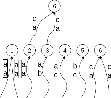 |
|
Recursive algorithm
Because of input consistency, . For , we have , and we give a recursive formulation for . First, we introduce some notation. Given , we call an -mer white if all its occurrences arrive at the same vertex. Otherwise, we call the -mer black. Let be the number of white -mers starting from any vertex in and reaching , and let be the set of all black -mers of length . Finally, let denote the maximal interval of vertices that we can reach starting from and following an -mer . Note that for two distinct black -mers and any , .
We compute by dividing the number of -mers reaching from into those whose first half is white, and those whose first half is black:
| (3) |
The first term of the sum avoids double counting because all the first white halves are different. The second term counts the number of -mers that reach with each black -mer as a prefix, starting from .
To fulfill the recursion, we run into the issue that for two -mers and and any interval , , and we cannot easily infer the value of from if . We settle for computing for all intervals at every level of the recursion, and for every . This requires a table of size at every level of the recursion, where each value takes time to compute with formula 3 once the terms inside the sum have been computed.
Once we have found all , the terms for the next recursion can be computed by subtracting the black -mers reaching the vertices, which we can check from the sets as shown in appendix B. There, we also show how to compute the intervals of -mers in and from the LCS array and the sets . Note that knowing the endpoints of the intervals of vertices reached by the -mers in is enough to fulfil the recursion. We achieve this by building a data structure of size that allows us to compute each from in time, to find the intervals of -mers in in time, and all in a total of time.
With recursion steps, we arrive at an algorithm with running time, and space. The space complexity can be achieved by only keeping in memory the table from the last iteration. All together, we have shown the following theorem:
Theorem 10.
We can compute the number of distinct -mers of a DWG in time , where .
5 -mer preserving graph transformations to Wheeler graphs
The algorithms in Section 4 are of limited usability since they apply only to deterministic Wheeler graphs. In this Section we discuss how to transform some more general graphs into deterministic Wheeler graphs.
An layered DAG with layers is a directed acyclic graph that can be partitioned into disjoint subsets of vertices such that edges exists only from vertices in into for . For any graph, we can build the times unfolded DAG, which preserves the -mers in the graph:
Definition 11.
The times unfolded DAG of a graph is a layered DAG with layers such that the vertices on each layer are a copy of the vertices of , and the edge set is defined so that for every edge in there are edges from the copy of in layer to the copy of in layer for all .
We can turn this into a DFA by introducing a new initial state with epsilon-transitions into the first layer, and determinizing with the classic subset construction. Now, since every -mer corresponds to a distinct path from the initial state to the final layer, we can count -mers by counting the distinct paths to each node on the final layer of the DAG, which is easily done with a dynamic programming algorithm that processes the nodes in topological order.
However, this does not exploit overlaps between -mers. For deterministic acyclic graphs that have a source node that can reach all nodes, we may use the Wheelerization algorithm of Alanko et al. [2] that computes the smallest equivalent Wheeler DFA in time in the size of the output. More generally, if the input is the state graph of any DFA recognizing a Wheeler language, the minimum equivalent Wheeler DFA can be constructed in time, where is the size of the output [8].
Another option is to build the de Bruijn graph of the -mers, which is always Wheeler [10]. Unfortunately, this does not help much with counting the -mers because building the de Bruijn graph takes time proportional to the number of -mers, since there is one node per -mer. That is, building the de Bruijn graph amounts to a brute force enumeration of all -mers. However, the de Bruijn graph is not necessarily the smallest graph for a given set of -mers: For example, the Wheeler DFA minimization algorithm of Alanko et al. [1], run on the de Bruijn graph, can reduce the size of the graph while maintaining Wheelerness. Building this compressed graph directly without first building the de Bruijn graph would be useful, but seems to be nontrivial. We leave this open for future work.
6 The de Bruijn Graph of a Deterministic Wheeler Graph
In this section, we define a representation of the node-centric de Bruijn graph of the -mers of a DWG , building on the definitions of black and white -mers and the counting algorithms introduced in the previous section. We denote the de Bruijn graph by . First, we describe the data structure contents, then we describe the algorithms to navigate the de Bruijn graph given this data structure, and then we analyse their time and space in bits. Finally we show how to build it in time and space . The main technical difficulty of this section is that each vertex may have exponentially many white -mers that reach only . Thus, to support de Bruijn graph navigation we need to keep track of the rank of the -mer among all the -mers reaching , and update it to the rank in another vertex as we traverse an edge.
6.1 Data structure
Before presenting the data structure components, we define some new concepts.
-
A left-extension of an -mer is an -mer , that has as a suffix. Note that all left-extensions of a white -mer are also white.
-
The left-contraction of an -mer is the maximal interval of vertices that reaches. The left-contraction of a white -mer may be black.
-
For a vertex , is the array containing the number of distinct left-extensions of each -mer reaching , sorted by their colex order.
-
For a vertex , the intervals and are defined as:
-
–
.
-
–
-
–
We give a few more details on the intervals. If any of or does not exist, we define the respective left or right interval to be empty. Furthermore, for an interval of vertices where , we note that by Corollary 7, and this -mer is black. We represent the intervals by the two endpoints . In the appendix we show how to compute the intervals for all and all in time, by scanning the vertices left-to-right and using the function in each level.
Components.
The data structure is comprised of the following parts:
-
The standard Wheeler index for [10].
-
For all , the -mer counts .
-
For all and all , with , a cumulative array where is the total number of -mers reaching that are smaller than .
-
For all , the intervals and , stored as described above.
Now, we describe how to implement the navigation queries with these data structures, and afterwards we analyse their space and time complexity.
6.2 de Bruijn Graph Navigation
The operations we implement return the handle of a -mer, listing outgoing labels from a -mer, and performing forward traversal with an outgoing label.
Handle of a -mer.
The handle of a -mer is a triple , where is the maximal interval of that reaches, and is the rank of in the colex order of -mers reaching the left endpoint . We obtain and via the standard forward-search on the Wheeler index, but we must keep track of the rank . For let be the interval of vertices that we obtain after matching , starting from . At any step where , because . If for some , we update as follows. We find the rank of among the in-neighbours of with the Wheeler index, and we set .
Listing outgoing labels.
Given a handle , with the standard Wheeler graph index we can output the distinct outgoing labels in time per label, using rank and select operations [10].
Forward traversal.
Given the handle of a -mer , , and a label , we can return the handle of by first performing a left contraction on , which returns an interval and then matching from that interval with the Wheeler index and updating the rank (this is done in the same way as when we return the handle of a full -mer).
To perform a left contraction we distinguish two cases. If , then the left contraction is equal to , and the rank is . If , then the rank of is equal to . If the new rank is or , then the interval is or , respectively. Otherwise, is a white -mer, and the interval is .
6.3 Analysis
We store the -mer counts and the arrays as arrays of integers. The required integer size is given by the maximum number of -mers, across all . We denote by the number of -mers of , and with this notation, we obtain that we require bits to store the counts . The integers in grow up to , thus we require bits to represent the arrays. The intervals take up bits. The Wheeler graph index is representable in bits [10].
Finally, to build the predecessor data structure on , we encode in unary, for example by , where is the operator for concatenation of bit sequences. We build the classic constant rank and select data structures on it [14, 6]. To analyse the space, observe that all left extensions counted by all arrays for all represent distinct -mers, except for at most shared -mers between the vertices. Therefore, the sum of all zeros in all is bounded by . The number of ones in corresponds to the number of -mers arriving at . Notice, however, that we only compute for non-sink vertices, thus for each distinct -mer represented by a -bit we have a distinct -mer in by right-extension. Thus, we get at most ones. The space becomes bits111Here we used [11]..
The time needed for the operations to obtain the handle of a -mer are bounded by Wheeler graph operations, which take each. Listing outgoing labels can be done in time per label. The forward traversal requires one Wheeler graph matching, and a predecessor on , which can be implemented now with constant time rank and select on . Therefore, we arrive at the following theorem:
Theorem 12.
There exists a data structure for simulating navigation of the de Bruijn graph of the -mers of a Wheeler graph , which uses bits of space. It implements retrieving the handle of a -mer in time, listing of outgoing labels in time per label, and forward traversal in time.
6.4 Computation of the data structure
We have discussed how to obtain the -mer counts of in section 4, from which we obtain and , and we obtain the left and right intervals as shown in appendix C. The Wheeler graph index is as in [10]. Computing the arrays is more challenging though, because its size is proportional to the number of -mers of , which can be exponential. We develop a recursive formula for in terms of , which if it were implemented directly, it would lead to a solution. Then, we show a smart dynamic program that implements it and computes in time and space.
6.4.1 Computation of
Let be an -mer, and denote by the number of left-extensions of that reach . First, we observe that all the -mers reaching can be found by appending to the set of -mers reaching the vertices of (formula 1). The same can be said about left extensions. We observe two facts:
-
1.
Let be an -mer reaching only one vertex , and assume it is the th -mer of . Then,
-
2.
Assume reaches a maximal range of in-neighbours , with . Then,
(4) where and . Note how we must avoid double-counting left-extensions of size that might reach several in-neighbours.
The second case can only happen for -mers that are the minimum or the maximum ones of an in-neighbour , by Corollary 7. Similarly, a “middle” -mer that is not or will always fall into case 1, where , that can be computed recursively. With these observations, we design an algorithm that computes for all in two steps. First, we compute all and for all and , which can be done in time, and can be used to compute the number of left extensions of -mers in case 2. Then, we use a recursive algorithm to report the middle values of . To implement these algorithms, we will need all -mer counts for all and , as well as the data structure to support queries and queries.
Computing and .
First, we observe that , and by input-consistency. Then, for , we compute as follows. First, we scan the in-neighbours left-to-right until finding the first one with a non-zero count of -mers. Let be this vertex. We add the count of left-extensions of the first -mer of , and in case that -mer is shared by more in-neighbours (which can be checked with ), updating the count as in equation (4) above for every in-neighbour that shares the -mer. The computation of is similar, but going right-to-left, starting from the rightmost in-neighbour that has . Clearly, we spend time per vertex per value of , thus in total we spend time, and obtain a data structure of size .
Computing the rest of recursively.
We sketch a recursive procedure called , that appends to one array the counts of left-extensions that we find for -mers of . This procedure uses too many recursive calls, which we fix in the next section.
We start by calling with and . Let . We scan the in-neighbours of left-to-right, and we find the first one with non-zero count of -mers, . We repeat the following steps for all in-neighbours starting from :
-
1.
Process the first -mer of . If we have counted its number of left-extensions already, ignore it. Otherwise, obtain the count of its left-extensions from the previously computed . If is shared with other in-neighbours, we have to apply formula (4) to count them. Append this count to . If we applied formula (4), we start again at step 1 with the last in-neighbour that has incoming. Otherwise, move to step 2.
-
2.
If , recurse on with a call to .
-
3.
Process the last -mer of . If is the last -mer of , stop. Otherwise, check . If it is false, we append to . If it is true, we compute the number of left-extensions of with formula (4), and we move to the last in-neighbour that has incoming.
It is possible to compute these steps for all in-neighbours of in time plus the time to make the recursive calls, by using the left and right intervals and the function. We leave the details in appendix C. Still, this procedure uses too many recursive calls, since for some and , may be called by many out-neighbours of . However, we observe that every such call outputs the exact same numbers to . Therefore, using dynamic programming with memoization we can avoid computing repeated sub-problems.
Memoization.
We build the -times unfolded graph , and we add to all the vertices of a placeholder for two pointers and . At the start of the algorithm, these pointers are empty. Crucially, we keep and reuse the pointers between computations of for different . We consider a call to as a call on the vertex at layer . Whenever we recurse on a vertex for the first time, we set to the next position in the current list , where the next value will be appended. When the recursion returns, is set to point to the last filled position in . The next time we recurse on , whether in the computation of or another , instead of running the algorithm, we output all values between and on .
Complexity.
Clearly, now there are at most recursions during the computation of all . These take time once per vertex, when the pointers and have not been computed yet. This amounts to time in total. All other time is spent reporting values of , which as we argued before, there are of them. We have finally showed the following theorem:
Theorem 13.
We can build the data structure for de Bruijn graph navigation on the -mers of a Wheeler graph , in time and space .
7 Conclusion
This work, to the best of our knowledge, is the first to study the problem of -mer counting on graphs. We have introduced the problem and established both hardness results and tractable cases. While the problem turns out to be P-hard, our results show that the problem is in P in the class of Wheeler graphs, and by extension on any class of graphs that can be transformed into a Wheeler graph of polynomial size, without changing the -mers. As the first application for our -mer counting algorithm, we have shown how to simulate the de Bruijn graph of the -mers of a Wheeler graph, without having to construct -mers explicitly, improving on the state-of-the-art in this respect [20].
The tractability of the problem on Wheeler graphs raises several natural open questions. First, can we find the smallest Wheeler graph that preserves the -mers of a given input graph? Second, which kinds of graphs admit polynomial-size Wheelerizations with the same -mer set? Third, what is the best achievable polynomial degree of for algorithms running in time on Wheeler graphs? This work thus marks a first step toward a broader theory of -mer counting in graphs.
References
- [1] Jarno Alanko, Nicola Cotumaccio, and Nicola Prezza. Linear-time minimization of wheeler dfas. In 2022 Data Compression Conference (DCC), pages 53–62. IEEE, 2022. doi:10.1109/DCC52660.2022.00013.
- [2] Jarno Alanko, Giovanna D’Agostino, Alberto Policriti, and Nicola Prezza. Regular languages meet prefix sorting. In Proceedings of the Fourteenth Annual ACM-SIAM Symposium on Discrete Algorithms, pages 911–930. SIAM, 2020. doi:10.1137/1.9781611975994.55.
- [3] Jarno N. Alanko, Davide Cenzato, Nicola Cotumaccio, Sung-Hwan Kim, Giovanni Manzini, and Nicola Prezza. Computing the LCP array of a labeled graph. In Shunsuke Inenaga and Simon J. Puglisi, editors, 35th Annual Symposium on Combinatorial Pattern Matching, CPM 2024, June 25-27, 2024, Fukuoka, Japan, volume 296 of LIPIcs, pages 1:1–1:15. Schloss Dagstuhl – Leibniz-Zentrum für Informatik, 2024. doi:10.4230/LIPIcs.CPM.2024.1.
- [4] Bahar Alipanahi, Alan Kuhnle, Simon J Puglisi, Leena Salmela, and Christina Boucher. Succinct dynamic de bruijn graphs. Bioinformatics, 37(14):1946–1952, July 2021. doi:10.1093/bioinformatics/btaa546.
- [5] Alexander Bowe, Taku Onodera, Kunihiko Sadakane, and Tetsuo Shibuya. Succinct de bruijn graphs. In Ben Raphael and Jijun Tang, editors, Algorithms in Bioinformatics, pages 225–235, Berlin, Heidelberg, 2012. Springer Berlin Heidelberg. doi:10.1007/978-3-642-33122-0_18.
- [6] David Richard Clark. Compact PAT trees. PhD thesis, University of Waterloo, Canada, 1996.
- [7] Alessio Conte, Nicola Cotumaccio, Travis Gagie, Giovanni Manzini, Nicola Prezza, and Marinella Sciortino. Computing matching statistics on wheeler dfas. In Proc. Data Compression Conference (DCC), pages 150–159. IEEE, 2023. doi:10.1109/DCC55655.2023.00023.
- [8] Giovanna D’Agostino, Davide Martincigh, and Alberto Policriti. Ordering regular languages and automata: Complexity. Theoretical Computer Science, 949:113709, 2023. doi:10.1016/J.TCS.2023.113709.
- [9] Johannes Fischer. Optimal succinctness for range minimum queries. In Alejandro López-Ortiz, editor, LATIN 2010: Theoretical Informatics, pages 158–169, Berlin, Heidelberg, 2010. Springer Berlin Heidelberg. doi:10.1007/978-3-642-12200-2_16.
- [10] Travis Gagie, Giovanni Manzini, and Jouni Sirén. Wheeler graphs: A framework for bwt-based data structures. Theoretical computer science, 698:67–78, 2017. doi:10.1016/J.TCS.2017.06.016.
- [11] Daniel Gibney and Sharma V. Thankachan. On the Complexity of Recognizing Wheeler Graphs. Algorithmica, 84(3):784–814, 2022. doi:10.1007/s00453-021-00917-5.
- [12] Torben Hagerup. Sorting and searching on the word ram. In Proc. 15th STACS, pages 366–398, 1998. doi:10.1007/BFB0028575.
- [13] Dov Harel and Robert Endre Tarjan. Fast algorithms for finding nearest common ancestors. SIAM Journal on Computing, 13(2):338–355, 1984. doi:10.1137/0213024.
- [14] Guy Joseph Jacobson. Succinct static data structures. PhD thesis, Carnegie Mellon University, USA, 1988.
- [15] Juha Kärkkäinen, Peter Sanders, and Stefan Burkhardt. Linear work suffix array construction. J. ACM, 53(6):918–936, 2006. doi:10.1145/1217856.1217858.
- [16] Toru Kasai, Gunho Lee, Hiroki Arimura, Setsuo Arikawa, and Kunsoo Park. Linear-time longest-common-prefix computation in suffix arrays and its applications. In Amihood Amir, editor, Combinatorial Pattern Matching, pages 181–192, Berlin, Heidelberg, 2001. Springer Berlin Heidelberg. doi:10.1007/3-540-48194-X_17.
- [17] Sung-Hwan Kim, Francisco Olivares, and Nicola Prezza. Faster Prefix-Sorting Algorithms for Deterministic Finite Automata. In Laurent Bulteau and Zsuzsanna Lipták, editors, 34th Annual Symposium on Combinatorial Pattern Matching (CPM 2023), volume 259 of Leibniz International Proceedings in Informatics (LIPIcs), pages 16:1–16:16, Dagstuhl, Germany, 2023. Schloss Dagstuhl – Leibniz-Zentrum für Informatik. doi:10.4230/LIPIcs.CPM.2023.16.
- [18] Udi Manber and Gene Myers. Suffix arrays: a new method for on-line string searches. siam Journal on Computing, 22(5):935–948, 1993. doi:10.1137/0222058.
- [19] Camille Marchet, Christina Boucher, Simon J Puglisi, Paul Medvedev, Mikaël Salson, and Rayan Chikhi. Data structures based on k-mers for querying large collections of sequencing data sets. Genome research, 31(1):1–12, 2021.
- [20] Jouni Sirén. Indexing variation graphs. In 2017 Proceedings of the ninteenth workshop on algorithm engineering and experiments (ALENEX), pages 13–27. SIAM, 2017. doi:10.1137/1.9781611974768.2.
- [21] Leslie G Valiant. The complexity of enumeration and reliability problems. siam Journal on Computing, 8(3):410–421, 1979. doi:10.1137/0208032.
Appendix A Proof of Lemmas 6 and 8
Lemma 6.
[Restated, see original statement.]
For two nodes in a DWG, if , then for any two -mers and such that and , we have .
Proof.
If , the claim is trivially true. Otherwise, let be the largest index such that . Let . There exists a path labeled with such that , and a path labeled with such that . We also have for all , or otherwise the graph is not deterministic, so we can iterate Lemma 2 for pairs of edges , , starting from to obtain . Since , if then W1) implies , a contradiction. Thus, it must hold that , which implies .
Lemma 8.
[Restated, see original statement.]
Two different nodes of a DWG share a -mer if and only if. In that case, is a suffix of , and is a suffix of .
Proof.
The lemma follows from two facts:
-
1.
and can only share a -mer if and ,
-
2.
implies that is a suffix of , and implies that is a suffix of .
Thus, if , then , and 2) implies . Otherwise, if , either a) , and 1) does not hold, so the -mers cannot be shared; or , but then by 2) and are suffixes of and , and then their LCS is less than .
For the proof, let be the set of left-infinite strings reaching , union with the set of finite strings starting at a source, and ending at . It is easy to check that the definitions of and in [3] are equivalent to and . Observe that if exists, there exists a maximum string in suffixed by : Let be the walk, possibly left-infinite, that is created right-to-left by following i) first the edges that form , and then ii) the maximum incoming edge to the last found vertex on the walk. This walk ends at and is either a left-infinite string, or starts in a source; thus it spells a string in , that is suffixed by . The same argument holds for a minimum string in suffixed by , following the smallest incoming edge.
We prove 2) first. Assuming that , let be the suffix of length of . We have that , because can always be chosen as . By contradiction, assume that . Now, consider the maximum string that is suffixed by : Since , then , but this contradicts . Similarly, if and is the suffix of length of , we have because we can choose . But if , then the minimum string suffixed by is strictly smaller than , a contradiction.
To prove 1), we show two intermediate claims:
-
A)
If exists, implies . To see why, let be the minimum string in suffixed by . We have because they are of different lengths, but , therefore . Since is a suffix of of length , but and , then we have .
-
B)
regardless of the length of . Let be the maximum string in suffixed by : Since is a suffix of , , and since , we have , which implies B).
Now, we have all the ingredients to prove 1): if , we have by A) and B) that , so the -mers cannot be shared. So we can assume , and by 2) is a suffix of . If , because of the length of , we have , and since is a suffix of , we have , that by B) implies . So, the only time when and can share a -mer is when and .
Appendix B Details of the algorithm
We show here how to compute and . We use the and functions, and the algorithm by Kim et al [17]. Given that we can compute the array in time [3], the and functions can be obtained directly from it and an RMQ data structure, as shown before (formula 2). The algorithm of Kim et al. constructs the sets at each iteration, that contain the vertices such that there exists a path spelling from to . We make a matrix of size , where if . Furthermore, we index the columns of for range maximum queries [9]. With this data structure, we can answer the following query: For an interval , define if there exists any such that starts at and ends at , otherwise . We can build the corresponding data structures for the suprema, to answer the following queries: if and only if starts at some and ends at . Now, we can compute with the following formula:
It takes time to compute for all and for both infima and suprema in each iteration. Then, we spend time to build the matrices and and their correspondent range maximum data structures. The queries take time. Thus, after time, we can compute in constant time from .
To compute for , we first compute all intervals by scanning the vertices left-to-right and looking for the maximal intervals of vertices that share an -mer, aided by the functions and (see a more detailed version in appendix C). Once we have them, we restrict all found intervals to the vertices reachable from as follows. Scanning left to right, we change the left endpoint of to the first vertex such that . Similarly, we change the last endpoint to the last vertex such that . Since there are such intervals, and their intersections are of size , this procedure can be done in time for a given interval . Across all intervals, we have a total of work.
Appendix C Computing intervals and left-extensions
First, we show how to compute all and for all vertices and all in time once we have the -mer counts. Then, we give the missing details for the left-extension counting algorithm of subsection 6.4.1.
Computing intervals.
For any , the sources have . For , the left and right intervals of any vertex are the same, and they correspond to the intervals of vertices with the same incoming label. For , first we find for every non-source if , by checking if . This is easy: if and only if .
Once we have this information, it is easy to run a loop through the non-source vertices, from smallest to largest, to find the maximal runs of vertices such that for all we have , and for all it holds that . With this information, we can find all maximal intervals of all the vertices and assign them correctly. The algorithm takes time for each vertex in each level, thus it takes time in total.
Computing left-extensions.
We left out some details on the recursive algorithm to compute left-extensions. For a vertex and an in-neighbour of , let and be the first and last -mers of , respectively. We clarify the following points:
-
How to compute formula 4 in time proportional to the number of in-neighbours that the -mer reaches. Note that this may be smaller than the size of the interval of that -mer.
-
How to keep track of whether we have counted the number of left-extensions of .
-
How to know if is the last -mer of .
For the first point, when reporting the number of left-extensions of the last -mer of , it may happen that is large, but it contains many vertices that are not in-neighbours of . To compute formula 4 efficiently, we get the right endpoint of , and we iterate the in-neighbours of starting from as long as they are smaller than . For each of them, we add the appropriate term to the sum, and we report the value at the end.
For the second point, we keep a variable throughout the algorithm, that indicates whether we should report the number of left-extensions of or not. At the start of the algorithm it is false, since the number of left-extensions of has been counted already (in ). When processing the last -mer of an in-neighbour , it may or may not be shared with more in-neighbours. If it is not shared, then is set to . Otherwise, if it is shared, and the last in-neighbour of that reaches has , then we set to , otherwise to .
For the last point, to avoid reporting the number of left-extensions , we have two cases. If we arrive at the last in-neighbour of , we just avoid running the last step of the algorithm. The other case is if, for some , it happens that contains , and . Thus, we must check every time we compute formula 4 if this is the case, and stop if so.