Efficient Index for Square Pattern Matching

($\Rightarrow$) Suppose that $X$ and $Y$ are square matched. By Definition 5, for every position $i$ and every $\mathrm{\ell }\ge 0$, the substring $X[i..i+2\mathrm{\ell }-1]$ is a square if and only if $Y[i..i+2\mathrm{\ell }-1]$ is a square. Hence, for each position $i$, the maximum such $\mathrm{\ell }$ is the same for $X$ and $Y$, implying that ${\mathrm{𝙻𝙿𝚂}}_X[i]={\mathrm{𝙻𝙿𝚂}}_Y[i]$. Therefore, ${\mathrm{𝙻𝙿𝚂}}_X={\mathrm{𝙻𝙿𝚂}}_Y$.

($\Leftarrow$) We prove this direction by induction on the string length $n$. Assume that ${\mathrm{𝙻𝙿𝚂}}_X={\mathrm{𝙻𝙿𝚂}}_Y$. For the base cases, when $n=1$, no square exists and ${\mathrm{𝙻𝙿𝚂}}_X={\mathrm{𝙻𝙿𝚂}}_Y=⟨0⟩$. When $n=2$, either ${\mathrm{𝙻𝙿𝚂}}_X={\mathrm{𝙻𝙿𝚂}}_Y=⟨0,0⟩$ or ${\mathrm{𝙻𝙿𝚂}}_X={\mathrm{𝙻𝙿𝚂}}_Y=⟨2,0⟩$. In the former case, both $X$ and $Y$ consist of two distinct characters; in the latter case, both consist of two identical characters. In either case, $X$ and $Y$ are square matched.

Assume that the statement holds for all , and consider the case $n=k$. Let $X^{\prime }$ and $Y^{\prime }$ denote the strings obtained from $X$ and $Y$ by removing their first character, respectively. Since the LPS array depends only on the suffixes starting at different positions, the last $k-1$ entries of ${\mathrm{𝙻𝙿𝚂}}_X$ coincide with those of ${\mathrm{𝙻𝙿𝚂}}_{X^{\prime }}$, and similarly for $Y$. Therefore, we have ${\mathrm{𝙻𝙿𝚂}}_{X^{\prime }}={\mathrm{𝙻𝙿𝚂}}_{Y^{\prime }}$. By the induction hypothesis, $X^{\prime }$ and $Y^{\prime }$ are square matched, which implies that $X[2..n]$ and $Y[2..n]$ are square matched.

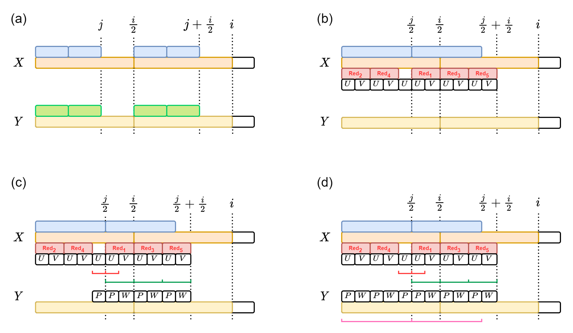
It remains to show that, for every $1\le h\le n$, the substring $X[1..h]$ is a square if and only if $Y[1..h]$ is a square. Let ${\mathrm{𝙻𝙿𝚂}}_X[1]={\mathrm{𝙻𝙿𝚂}}_Y[1]=i$. For every $i\le h\le n$, the substring $X[1..h]$ is a square if and only if $Y[1..h]$ is a square by Definition 8, and the statement holds trivially. For every , we prove the claim by contradiction. Without loss of generality, suppose that $X[1..j]$ is a square while $Y[1..j]$ is not. We separate the discussion into two cases, which together cover all possibilities.

To give a better illustration, we will use several figures as an aid. In these figures, we use Color to represent substrings in the figures. For instance, Yellow denotes the substring colored in yellow. Substrings sharing the same color represent identical strings, and additional labels are sometimes used to distinguish different occurrences of the same substring.

As shown in Figure 3(a), since $X[1..i]$ is a square, it follows that

Hence, the substring $X[\frac{i}{2}+1..\frac{i}{2}+j]$ is also a square.By the induction hypothesis, $Y[\frac{i}{2}+1..\frac{i}{2}+j]$ is a square as well. Moreover, since $Y[1..i]$ is a square, it follows that $Y[1..j]$ is a square, contradicting our assumption.

As shown in Figure 3(b), we have the following three squares:

Square 1:

$X[1..\frac{j}{2}]=X[\frac{j}{2}+1..j]$.

Square 2:

$X[1..\frac{i}{2}]=X[\frac{i}{2}+1..i]$.

Square 3:

$Y[1..\frac{i}{2}]=Y[\frac{i}{2}+1..i]$.

Note that identical substrings are colored in the same color. To distinguish different occurrences of the same-colored substrings, we will use subscripts, such as ${\text{Red}}_1$, ${\text{Red}}_2$, and so on, for different substrings in red.

We first focus on the substring $X[\frac{j}{2}+1..\frac{i}{2}]$ (denoted by ${\text{Red}}_1$). By Square 1, ${\text{Red}}_2$ occurs as a prefix of $X$. Applying Square 2 and Square 1 repeatedly, we obtain ${\text{Red}}_3$ (by Square 2) and ${\text{Red}}_4$ (by Square 1). We continue this process until we obtain a substring whose ending position is greater than or equal to $j$ (denoted by ${\text{Red}}_5$ in the example).

We divide ${\text{Red}}_5$ at position $j$ into two substrings, denoted by $U$ and $V$, and replace all occurrences of Red accordingly, as shown in Figure 3(b). We observe that there are multiple squares composed of $U$ and $V$. These squares are marked by brackets of different colors in Figure 3(c). By the induction hypothesis, the corresponding substrings of $Y$ are also squares and can be decomposed into $P$ and $W$.

Finally, as shown in Figure 3(d), a sequence of $P$ and $W$ appears as a prefix of $Y$ by Square 3. As indicated by the pink brackets, we have $Y[1..\frac{j}{2}]=Y[\frac{j}{2}+1..j]$, which implies that $Y[1..j]$ is a square, contradicting our assumption.

The case where $V$ is empty, that is, when ${\text{Red}}_5$ ends exactly at position $j$, can be proved analogously and is therefore omitted.

In summary, both cases lead to a contradiction, and the proof completes. $◀$

Observe that the LPS array of $S[i+1..i+\mathrm{\ell }]$ coincides with the last $\mathrm{\ell }$ entries of the LPS array of $S[i..i+\mathrm{\ell }]$. This observation motivates the use of a two-dimensional table, called the LPS table ($\mathrm{\Lambda }[1..n][1..n]$), to store the LPS arrays of all substrings of $S$.

An example is illustrated in Figure 2(b). In particular, to reconstruct the LPS array of the substring $S[i..i+\mathrm{\ell }-1]$, we consider the following diagonal of the LPS table:

The LPS table of $S$ requires $n^2\lg n$ bits of space to store and can be constructed in $O(n^2)$ time.¹¹1In practice, the space can be reduced by a factor of two by storing only rows corresponding to even lengths, since $\mathrm{\Lambda }[\mathrm{\ell }][i]=\mathrm{\Lambda }[\mathrm{\ell }-1][i]$ for all odd $\mathrm{\ell }$. We defer the construction of the LPS table to Section 4.2.

Since the LPS table of $S$ contains the LPS arrays of all substrings of $S$, we can answer ${\text{Loc}}_{\text{sqr}}(S,P)$ by locating ${\mathrm{𝙻𝙿𝚂}}_P$ among those represented in the LPS table of $S$. To support this operation efficiently, we construct an additional data structure: a trie built over all diagonals of the LPS table of $S$. Equivalently, this trie stores the LPS arrays of all prefixes of $S$.

Note that the edges of the diagonal trie only store references to entries of the LPS table; thus, access to the LPS table must be available. The following lemma summarizes the space usage of the diagonal trie and its construction time.

The diagonal trie is a compressed trie containing $n$ leaves, one for each diagonal of the LPS table (equivalently, one for each position of $S$). In a compressed trie, every internal node except the root has degree at least two. Hence, the number of internal nodes is at most $n-1$, and the total number of nodes and edges is $O(n)$.

Each node and edge stores indices or pointers of size $O(\lg n)$ bits. Since the total number of nodes and edges is $O(n)$, the trie itself occupies $O(n\lg n)$ bits. Moreover, the deterministic static dictionaries for the outgoing edges also require $O(n\lg n)$ bits in total. Therefore, the diagonal trie requires $O(n\lg n)$ bits of space.

To construct the trie, we insert all $n$ diagonals of the LPS table. The total length of all diagonals is ${\sum }_{i=1}^{n}i=O(n^2)$, and thus the total insertion time is $O(n^2)$. Since each node is augmented with a deterministic static dictionary, and the total number of entries across all these dictionaries is $O(n)$, constructing all deterministic static dictionaries requires $O(n^{1+ϵ})$ time [16] for any constant $ϵ>0$. We will choose . Since $O(n^{1+ϵ})=o(n^2)$, this does not affect the overall time bound. Therefore, the construction time is $O(n^2)$. $◀$

Up to this point, the LPS index of $S$ consists of the following two components:

1. 1.

   the LPS table of $S$;

2. 2.

   the diagonal trie of the LPS table.

To answer ${\text{Loc}}_{\text{sqr}}(S,P)$, we first compute ${\mathrm{𝙻𝙿𝚂}}_P$, and then traverse the diagonal trie of $S$ by scanning ${\mathrm{𝙻𝙿𝚂}}_P$ from right to left. If the traversal succeeds and terminates at a node (which may be an implicit node located in the interior of an edge), then for each leaf in the subtree rooted at this node, we insert the position $i-|P|+1$ into ${\text{Loc}}_{\text{sqr}}(S,P)$, where $i$ is the position stored at the leaf. Otherwise, we return the empty set.

We summarize the query time complexity of the above procedure as follows.

Each node of the diagonal trie stores its outgoing edges in a deterministic static dictionary supporting worst-case $O(1)$ query time [16]. Thus, retrieving the next edge during traversal takes $O(1)$ time. Querying the pattern $P$ traverses at most $m$ nodes, resulting in a total time of $O(m)$. Traversing all leaves in the corresponding subtree takes $O(\text{occ})$ time. If the array ${\mathrm{𝙻𝙿𝚂}}_P$ is not given, it can be computed in $O(m\lg m)$ time using Algorithm 1. Therefore, the overall time complexity is $O(m\lg m+\text{occ})$. $◀$

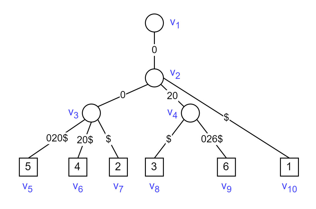
An example is illustrated in Figure 2(c). The blue labels $v_i$ denote the node indices. Given $P=\text{cdd}$, we have ${\mathrm{𝙻𝙿𝚂}}_P=⟨0,2,0⟩$. We start from the root ($v_1$), follow the edges to traverse $v_2$, and eventually reach $v_4$. From here on, we know that each leaf in the subtree rooted at $v_4$ witnesses a substring matching with $P$. Each leaf stores the ending position of this substring, so subtracting $|P|-1$ from this ending position gives the starting position of the matching substring. By doing this for each leaf in this example, we form the set ${\text{Loc}}_{\text{sqr}}(S,P)=\{1,4\}$.

References

- [1] Amihood Amir, Richard Cole, Ramesh Hariharan, Moshe Lewenstein, and Ely Porat. Overlap matching. Inf. Comput., 181(1):57–74, 2003. doi:10.1016/S0890-5401(02)00035-4.
- [2] Brenda S. Baker. Parameterized Pattern Matching: Algorithms and Applications. J. Comput. Syst. Sci., 52(1):28–42, 1996. doi:10.1006/JCSS.1996.0003.
- [3] Hideo Bannai, Tomohiro I, Shunsuke Inenaga, Yuto Nakashima, Masayuki Takeda, and Kazuya Tsuruta. The "Runs" Theorem. SIAM J. Comput., 46(5):1501–1514, 2017. doi:10.1137/15M1011032.
- [4] Maxime Crochemore and Wojciech Rytter. Squares, Cubes, and Time-Space Efficient String Searching. Algorithmica, 13(5):405–425, 1995. doi:10.1007/BF01190846.
- [5] Maxime Crochemore and Wojciech Rytter. Jewels of stringology: text algorithms. World Scientific, 2002.
- [6] Jonas Ellert and Johannes Fischer. Linear Time Runs Over General Ordered Alphabets. In 48th International Colloquium on Automata, Languages, and Programming, ICALP 2021, Glasgow, Scotland (Virtual Conference), July 12-16, 2021, pages 63:1–63:16. Schloss Dagstuhl – Leibniz-Zentrum für Informatik, 2021. doi:10.4230/LIPIcs.ICALP.2021.63.
- [7] Michael Fredman and Dan Willard. Blasting through the information theoretic barrier with fusion trees. In ACM Symposium on Theory of Computing, pages 1–7, 1990. doi:10.1145/100216.100217.
- [8] Garance Gourdel, Tomasz Kociumaka, Jakub Radoszewski, Wojciech Rytter, Arseny M. Shur, and Tomasz Walen. String periods in the order-preserving model. Inf. Comput., 270, 2020. doi:10.1016/J.IC.2019.104463.
- [9] Diptarama Hendrian. Generalized Dictionary Matching Under Substring Consistent Equivalence Relations. In WALCOM: Algorithms and Computation (WALCOM 2020), volume 12049 of Lecture Notes in Computer Science, pages 120–132. Springer, 2020. doi:10.1007/978-3-030-39881-1_11.
- [10] Tomohiro I, Shunsuke Inenaga, and Masayuki Takeda. Palindrome pattern matching. Theor. Comput. Sci., 483:162–170, 2013. doi:10.1016/J.TCS.2012.01.047.
- [11] Jinil Kim, Peter Eades, Rudolf Fleischer, Seok-Hee Hong, Costas S. Iliopoulos, Kunsoo Park, Simon J. Puglisi, and Takeshi Tokuyama. Order-preserving matching. Theor. Comput. Sci., 525:68–79, 2014. doi:10.1016/J.TCS.2013.10.006.
- [12] Donald E. Knuth, James H. Morris Jr., and Vaughan R. Pratt. Fast Pattern Matching in Strings. SIAM J. Comput., 6(2):323–350, 1977. doi:10.1137/0206024.
- [13] Roman M. Kolpakov and Gregory Kucherov. Finding Maximal Repetitions in a Word in Linear Time. In 40th Annual Symposium on Foundations of Computer Science, FOCS 1999, New York, NY, USA, October 17-18, 1999, pages 596–604. IEEE Computer Society, 1999. doi:10.1109/SFFCS.1999.814634.
- [14] Xingyu Liao, Wufei Zhu, Juexiao Zhou, Haoyang Li, Xiaopeng Xu, Bin Zhang, and Xin Gao. Repetitive DNA sequence detection and its role in the human genome. Communications biology, 6(1):954, 2023. doi:10.1038/s42003-023-05322-y.
- [15] Yoshiaki Matsuoka, Takahiro Aoki, Shunsuke Inenaga, Hideo Bannai, and Masayuki Takeda. Generalized pattern matching and periodicity under substring consistent equivalence relations. Theor. Comput. Sci., 656:225–233, 2016. doi:10.1016/J.TCS.2016.02.017.
- [16] Peter Bro Miltersen. Error Correcting Codes, Perfect Hashing Circuits, and Deterministic Dynamic Dictionaries. In Proceedings of the Ninth Annual ACM-SIAM Symposium on Discrete Algorithms (SODA), pages 556–563. SIAM, 1998. URL: http://dl.acm.org/citation.cfm?id=314613.314845.
- [17] Shinya Nagashita and Tomohiro I. PalFM-Index: FM-Index for Palindrome Pattern Matching. In 34th Annual Symposium on Combinatorial Pattern Matching (CPM 2023), volume 259 of LIPIcs, pages 23:1–23:15. Schloss Dagstuhl – Leibniz-Zentrum für Informatik, 2023. doi:10.4230/LIPIcs.CPM.2023.23.
- [18] Sung Gwan Park, Amihood Amir, Gad M. Landau, and Kunsoo Park. Cartesian Tree Matching and Indexing. In 30th Annual Symposium on Combinatorial Pattern Matching (CPM 2019), volume 128 of LIPIcs, pages 16:1–16:14. Schloss Dagstuhl – Leibniz-Zentrum für Informatik, 2019. doi:10.4230/LIPIcs.CPM.2019.16.
- [19] Mihai Pătraşcu and Mikkel Thorup. Dynamic Integer Sets with Optimal Rank, Select, and Predecessor Search. In 55th IEEE Annual Symposium on Foundations of Computer Science, FOCS 2014, Philadelphia, PA, USA, October 18-21, 2014, pages 166–175. IEEE Computer Society, 2014. doi:10.1109/FOCS.2014.26.
- [20] Jouni Paulus and Anssi Klapuri. Music structure analysis by finding repeated parts. In Proceedings of the 1st ACM Workshop on Audio and Music Computing Multimedia, pages 59–68. Association for Computing Machinery, 2006. doi:10.1145/1178723.1178733.
- [21] Jouni Paulus, Meinard Müller, and Anssi Klapuri. State of the Art Report: Audio-Based Music Structure Analysis. In International Society for Music Information Retrieval Conference (ISMIR 2010), pages 625–636. ISMIR, 2010. URL: http://ismir2010.ismir.net/proceedings/ismir2010-107.pdf.
- [22] Siwoo Song, Geonmo Gu, Cheol Ryu, Simone Faro, Thierry Lecroq, and Kunsoo Park. Fast algorithms for single and multiple pattern Cartesian tree matching. Theor. Comput. Sci., 849:47–63, 2021. doi:10.1016/J.TCS.2020.10.009.