On the Fragile Complexity of Geometric Algorithms

In this paper, every problem we consider takes as input an array or list of items, such as numbers, points, or lines, which have real-valued attributes such as coordinates. Unless otherwise stated, the algorithms use the real RAM model of computation (without floors or ceilings) where decisions are made based on the signs of bounded-degree polynomials in the input attributes. The lower bounds use algebraic decision trees; see [11] for an overview. For some problems, we use a more restricted model.

Fix a specific algorithm solving a given problem, which stays in the algebraic decision tree/real RAM model. Consider the tree representing all possible computation and decision paths of the execution of the algorithm. The fragility of an item along an execution path is the number of operations it is involved in. The worst-case fragility of an item is the maximum number of operations it is involved in, along all possible executions paths. The fragility of the algorithm is the maximum fragility of any of the input items.

As we are also interested in the total work (or “cost” or “running time”) of our algorithm, we additionally measure the total number of real RAM operations performed along a worst-case execution path. For a randomized algorithm, we also examine the expected cost and fragility. We summarize the prior work next, and then state our problems and results.

Prior work on fragile complexity has focused on comparison-based algorithms [1] and adaptive algorithms [5]. We utilize the following results from [1] in our work:

Minimum: Given a list $X=⟨x_1,x_2,\mathrm{\dots },x_n⟩$ of $n$ numbers, find the smallest number, only allowing comparisons of the form ; more precisely, return $\arg {\min }_i{x}_i$. If numbers repeat, return the index of one smallest.

The upper bound in Theorem 2.1 comes from computing the minimum via tournament tree.

Sorting: Given a list $X=⟨x_1,x_2,\mathrm{\dots },x_n⟩$ of $n$ numbers, find a permutation $\sigma$ of the indices $⟨1,\mathrm{\dots },n⟩$ so that $x_{\sigma (1)}\le x_{\sigma (2)}\le \mathrm{\cdots }\le x_{\sigma (n)}$.

As a warmup for fragility, here is a proof of the Sorting fragility lower bound: Sorting has a lower bound of $\mathrm{\Omega }(n\log n)$ comparisons in the algebraic decision tree model. By the pigeonhole principle, the fragility of some element must be $\mathrm{\Omega }(\log n)$.

We obtain results on the following geometric problems on sets of points through the lens of fragile complexity. To our knowledge, this has not been done before.

Staircase: The staircase of a list of points $P$ is the $x$-ordered sequence of points in $P$ where no other point has both a larger $x$- and a larger $y$-coordinate. Given a list of $P=⟨p_1,\mathrm{\dots },p_n⟩$ points, output the sequence of indices of the staircase of $P$.

Closest Pair: Given a list $P=⟨p_1,p_2,\mathrm{\dots },p_n⟩$ of $n$ points in the plane, find the closest pair among them. More precisely, return a pair $(i,j)$ of indices so that $d(p_i,p_j)={\min }_{i^{\prime }\ne j^{\prime }}\{d(p_{i^{\prime }},p_{j^{\prime }})\}$.

Convex Hull: The convex hull is the smallest convex set enclosing a set of points. Given a list $P=⟨p_1,\mathrm{\dots },p_n⟩$ of points, produce the vertices of the convex hull of $P$ in counterclockwise order.

Triangulation: A triangulation of a point set is a subdivision of its convex hull into triangles whose edges form a maximal set of non-crossing segments connecting pairs of points. Given a set $P=⟨p_1,\mathrm{\dots },p_n⟩$ of points, produce a triangulation of the point set.

Approximate Euclidean MST: The Euclidean Minimum Spanning Tree (EMST) of a point set $P$ is a spanning tree of $P$ whose edges have minimum total length among all spanning trees on $P$, where the length of an edge is the Euclidean (${\mathrm{\ell }}_2$) distance between its vertices. A $c$-approximate EMST (apx-EMST) is a spanning tree of $P$ whose total length is at most $c$ times the length of the EMST. Given a set $P=⟨p_1,p_2,\mathrm{\dots },p_n⟩$ of $n$ points in the plane, find an approximate Euclidean MST, for some $c\ge 1$.

Our results are given in the table below. Our bounds for staircase are tight; a logarithmic gap remains in the other problems.

Note that the last lower bound is for the exact Euclidean MST. Observe that, somewhat surprisingly, we can achieve polylogarithmic fragility for computing a triangulation potentially containing high-degree vertices.

1. 1.

   Sort the points in $P$ in lexicographic order.

2. 2.

   We now proceed recursively.

   1. (a)

      Divide $P$ at the median into $P_{\text{left}}$ and $P_{\text{right}}$.

   2. (b)

      Recursively find the staircase $s_{\text{left}}$ of $P_{\text{left}}$ and the staircase $s_{\text{right}}$ of $P_{\text{right}}$.

   3. (c)

      Let $p_{\text{left}}$ be the point of $P_{\text{left}}$ corresponding to the first index of $s_{\text{left}}$ and $p_{\text{right}}$ the point of $P_{\text{right}}$ corresponding to the first index of $s_{\text{right}}$. If , return $s_{\text{right}}$.

   4. (d)

      Otherwise, binary search for $y(p_{\text{right}})$ (the key) among the points corresponding to $s_{\text{left}}$. Return the section of $s_{\text{left}}$ containing points with $y$-coordinate at least that of $y(p_{\text{right}})$, followed by $s_{\text{right}}$.

Step 1, presorting, uses $O(\log n)$ fragility [3] and costs $O(n\log n)$ running time (this step is the bottleneck).

We argue that each point of the set $P$ is involved in a logarithmic number of comparisons over the entire runtime of the recursive algorithm. Each point of $P$ participates in a logarithmic number of subproblems. Step 2(a) makes no comparisons. Step 2(c) involves one comparison between two points of the current subproblem and therefore causes at most logarithmic fragility.

It remains to bound the fragility arising from the binary search in Step 2(d). Each binary search comparison is between a key and an element of the current subproblem; the latter participates in one comparison per binary search and therefore a logarithmic number of comparisons overall. The key ($y(p_{\text{right}})$) is compared a logarithmic number of times in a fixed binary search. The binary search is only triggered once for each possible $p_{\text{right}}$ (when it is the topmost point of $P_{\text{right}}$, but not the topmost point in $P$). It will no longer be $p_{\text{right}}$ at higher levels of recursion. Hence it only participates in a logarithmic number of comparisons in its capacity as a key, completing the proof of logarithmic fragility. $◀$

In [17, Lemma 2.2] it was argued that a comparison-model decision tree for solving the Maxima problem must have at least $n!$ leaves and therefore requires $\mathrm{\Omega }(n\log n)$ comparisons. In the algebraic decision tree model, Kirkpatrick and Seidel give a lower bound of $\mathrm{\Omega }(n\log h)$ [15] for Maxima, where $h$ is the number of maxima. By the pigeonhole principle, and because $h=\mathrm{\Theta }(n)$ in the worst case, we obtain a lower bound of $\mathrm{\Omega }(\log n)$ on fragility of Maxima.

We will follow the $O(n\log n)$-time closest-pair divide-and-conquer algorithm from [8], with adjustments for fragility. Assume we are given an array $P$ of points $p_i=(x,y)$. The following are the steps our algorithm takes.

1. 0.

   Pre-sort the points of $P$, once by $x$-coordinate and once by $y$-coordinate, storing them in arrays $X$ and $Y$, respectively. Each point “knows” its position in these two arrays. That is, $X[i]$ not only stores the point of $P$ with $i$th largest $x$-coordinate, but also its position in the $Y$ array, and vice versa.

2. 1.

   Divide the array $X$ into two parts, $X_L$ and $X_R$, of nearly equal size partitioned by the median $x$-coordinate $x_m$. Let $Y_L$ and $Y_R$ denote the corresponding array of points, sorted by $y$-coordinate – they can be computed from $Y$ in linear time using the cross links mentioned above.

3. 2.

   Recursively solve Closest Pair (starting at step 1) on $(X_L,Y_L)$ and $(X_R,Y_R)$, which return closest pairs $(p_L,q_L)$ and $(p_R,q_R)$, respectively. Let $(p,q)$ be the pair that defines the smaller distance between these two pairs and let $\delta =d(p,q)$.

4. 3.

   Consider the strip of width $2\delta$ centered at the line $x=x_m$. We identify the points of $P$ lying in this strip in the following fragility-sensitive manner (recall that we cannot store the value $\delta$, but need to refer to $p$ and $q$ as necessary; we also need to watch the fragility of $x_m$). Specifically, we find the smallest index $i_L$ in $X$ so that (if it exists), by binary search. Similarly, we find the largest index $i_R$ in $X$ so that . The portion $X[i_L\mathrm{\dots }{i}_R]$ contains precisely the points of $P$ in the desired strip.

5. 4.

   We can extract the points of $X[i_L,\mathrm{\dots },i_R]$ into an array $F$ ordered by $y$-coordinate by scanning through $Y$ once and collecting points whose position in $X$ lies in $[i_L,i_R]$.

6. 5.

   As discussed in [8], any pair of points at distance less than $\delta$ from each other will appear at most seven places apart in $F$. Therefore, we now collect the following list of point pairs: a point $F[i]$ and a point $F[j]$ at most 7 positions beyond it, i.e., with . This produces no more than $7n$ pairs of points. We can now apply SampleMinimum from [1] to this list of pairs, to find the smallest distance defined by one them.

7. 6.

   We return the pair with smaller of two distances: $\delta =d(p,q)$ and the closest pair from step 5.

Step 0 (presorting) costs $O(\log n)$ fragility using the AKS sorting network [3].

The algorithm then proceeds by divide and conquer with $O(\log n)$ levels. Step 1 does not require access to point coordinates. We will show through analysis of the further steps that step 2 requires $O(\log n)$ fragility. Step 3 (or computing $i_L$ and $i_R$) involves binary search, which costs $O(\log n)$ fragility for points $p$ and $q$ and coordinate $x_m$; the other points potentially touched in binary search cost $O(1)$ fragility per point. Step 4 (creating the array $F$) involves constant fragility per point. For step 5, each point in $F$ participates in $O(1)$ pair comparisons (by the geometric analysis in [8]). Utilizing the minimum algorithm from [1] in step 5 allows us to calculate the overall minimum with expected $O(\log n)$ fragile complexity – each value comparison in minimum computation translates to a comparison of two distances between points in $P$. Generating the solution pair in step 6 involves $O(1)$ fragility.

Since we can guarantee $O(\log n)$ fragility at each level of recursion, and it is possible that the same pair of points is the closest at all $\log n$ levels of recursion, the overall fragile complexity is $O({\log }^{2}n)$. $◀$

Note that the fragility analysis of the above algorithm is tight in the worst case. Some points will participate in $\mathrm{\Omega }({\log }^{2}n)$ operations. Indeed, consider a point set whose size $n$ is a power of 2, in which the leftmost two points $(p_1,p_2)$ define the smallest distance $d$. Furthermore, make sure that that the $x$-separation between any other pair of points is larger than $d$. Then $(p_1,p_2)$ will be the solution of the leftmost subproblem on all levels of recursion and will be involved in a logarithmic number of binary search comparisons at each level.

We give a fragility-preserving reduction from Minimum to Closest Pair in the CP-model. This will show not only that Closest Pair has $\mathrm{\Omega }(\log n)$ fragile complexity, but also the closest pair of points experiences $\mathrm{\Omega }(\log n)$ fragility.

We start with an instance $X$ of Minimum, which is a list consisting on $n$ distinct numbers $x_i$, satisfying two additional constraints. We assume that $X\subset [0,0.1]$ and that, for any two values, $x_i$ and $x_j$ (with $i\ne j$), either $x_i>2x_j$ or $x_j>2x_i$. Map each $x_i$ to two points $p_{2i}=(0,{100}^i)$ and $p_{2i+1}=(x_i,{100}^i)$. This transforms an instance $X$ of Minimum, with $n$ numbers, to an instance $P=P(X)=⟨p_0,\mathrm{\dots },p_{2n-1}⟩$ of Closest Pair, with $2n$ points.

Consider any algorithm $A$ that solves Closest Pair using only the comparisons mentioned. Note that we never need to actually compute the distance from a point to itself or compare the distance defined a pair of points to itself: the answer is known without performing the calculation. Consider an instance $X$ to Minimum subject to the above constraints, transform it into an instance $P=P(X)$ of Closest Pair according to the mapping above, and run $A$ on $P$. We start with an immediate fact.

Two points in $P$ are twins if they come from the same number in $X$, i.e., they are points $p_{2r}$ and $p_{2r+1}$ for some $r$, $0\le r\le n-1$.

By ˜4.2(b)&(c), the smallest distance must correspond to some pair $(p_{2r},p_{2r+1})$ of twins. But $d(p_{2r},p_{2r+1})=x_r$, for all $r$, and thus the smallest distance in $P$ corresponds to the minimum in $X$, completing the proof. $\mathrm{⊲}$

If $k=l$, $p_k$ and $p_l$ are the same point, and the comparison can be resolved by one comparison, . If $i=j$, the comparison evaluates to true. If both $k=l$ and $i=j$, the comparison evaluates to false. So we assume $k\ne l$ and $i\ne j$ below.

In other words, $i=2r$ and $j=2r+1$, or vice versa. Then $d(p_k,p_l)=x_r$, and the comparison is equivalent to .

Recall that we assumed a “gap”: for any two numbers $x_a,x_b\in X$, if , then $x_a>2x_b$; and if , then $x_b>2x_a$; otherwise $x_a=x_b$.

Suppose $x_i>x_j$ and therefore $x_i>2x_j$, is true. With one comparison of $x_i$ and $x_j$ exhausted, we compare $x_i$ and $x_r$ to check if $x_i>x_r$ (and therefore $x_i>2x_r$). If this comparison returns true, adding the two inequalities gives us $x_i>x_j+x_r$, implying that the original inequality of is false, so we are done in two comparisons. Otherwise, $x_r>2x_i$ or $x_r=x_i$. In both cases, is true; two comparisons are enough.

If $x_i>x_j$ is false, we check if $x_j>2x_i$ by comparing $x_i$ and $x_j$. Since $x_j+r>2x_i+r$, the original comparison evaluates to true. Otherwise $x_i=x_j$, which we don’t need to check – the original comparison evaluates to true.

Suppose $p_k$ and $p_l$ are not twins. Then, by (c) of ˜4.2, $d\ge 99$. Since $x_i-x_j\in [0,0.1]$, the comparison evaluates to false. $◀$

˜4.2 implies that if $p_i,p_j,p_k,p_l$ have three or four distinct $y$-coordinates among them, the comparison can be resolved by just examining the $y$-coordinates, which are determined by the indices $i,j,k,l$. So it remains to handle cases where only two distinct $y$-coordinates appear among these, not necessarily distinct points. Note that we do not need to address the case of one $y$-coordinate, as that means at most two distinct points are involved in the distance comparison, which can be resolved without examining $x$-coordinates. Additionally, if there are no twins and exactly two distinct $y$-coordinates, the two pairs of points in the comparison are the same. Below are the remaining cases.

Suppose $p_i$ and $p_j$ are twins ($i=2r$ and $j=2r+1$, or vice versa) and $p_k$ and $p_l$ are twins ($k=2s$ and $l=2s+1$, or vice versa). Then $d(p_i,p_j)=x_r$, $d(p_k,p_l)=x_s$, so the comparison is equivalent to , as claimed. Now suppose $p_i$ and $p_k$ are twins and $p_j$ and $p_l$ are twins. If $p_i$ and $p_j$ are even and $p_k$ and $p_l$ are odd, so that $i=2r$ and $k=2r+1$ and $j=2s$ and $l=2s+1$, then $d(p_k,p_l)$ is greater than $d(p_i,p_j)$ as it involves a positive $x$-coordinate difference, while $d(p_i,p_j)$ does not, so is true. Now suppose $p_i$ is even and $p_j$ is odd and $p_k$ is odd and $p_l$ is even. Then $i=2r$, $j=2s+1$, $k=2r+1$, $l=2s$ and the distance comparison is equivalent to . Similar reasoning applies if $(i,j),(k,l)$ pairs are interchanged.

If there is one pair of twins and two $y$-coordinates, then the comparison involves the same point, $p$, on both sides, and two other points. Suppose $i=2s$, $k=j=2r+1$, and $l=2s+1$: without loss of generality, $p_i$ and $p_l$ are twins, and $p=p_j=p_k$ with an odd index. Then the $y$-coordinate differences cancel out on both sides, and the comparison of distances reduces to , which can be resolved by comparing $x_r$ to $x_s$, since by our assumption, either or . If $j=k$ is even, we have $i=2s$, $k=j=2r$, and $l=2s+1$, which resolves to , which is true. $◀$

We call a comparison of the two forms above on $P(X)$ useful if it reduces to at most two comparisons of two elements in $X$; refer to the lemmas above. Any other comparison does not depend on the $x_i$ values; we refer to these as useless comparisons.

An execution of $A$ for Closest Pair on $P(X)$ can be used to solve Minimum on $X$ by removing useless comparisons (i.e., resolving them without accessing $X$) and turning useful distance comparisons into comparisons between numbers of $X$. Note that the transformation preserves fragility as it does not require access to $X$ – we do not explicitly construct $P(X)$, but rather simulate each operation of $A$ on its points by translating them to operations on point indices and comparisons of elements in $X$.

Note that we could also obtain an $\mathrm{\Omega }(\log n)$ lower bound on fragility in the algebraic decision tree model (if we reduce, for example, from Element Uniqueness to Closest Pair in one dimension, to Closest Pair) [20], since this requires $\mathrm{\Omega }(n\log n)$ operations and thus $\mathrm{\Omega }(\log n)$ fragility, by pigeonhole principle. However, such reasoning does not yield any information about the fragility of the closest pair itself, which is why we provided the alternate reduction above.

We follow the exponential-then-binary search approach for the merge portion of mergesort used in [1], adapted to the geometry of convex hulls. In the exponential portion, we start with the rightmost point $q_1$ of $\mathrm{UCH}(Q)$ and the leftmost point $r_1$ of $\mathrm{UCH}(R)$, $q_1{r}_1$ being a tentative bridge between the two upper hulls. The goal is to identify a tangent point $r_l$ for $q_1$. In the exponential portion of the search, we fix $q_1$ and then, starting with $r_1=r_{2^0}$, we examine points $r_{2^k}$, for $k=0,1,2,\mathrm{\dots }$, until we find $k$ for which $q_1{r}_{2^k}{r}_{2^k+1}$ is oriented clockwise. If $q_1{r}_{2^k-1}{r}_{2^k}$ is also oriented clockwise, $r_l=r_{2^k}$ – we found the tangent for $q_1$. Otherwise, the desired tangent point $r_l$ for $q_1$ lies between $r_{2^{k-1}}$ and $r_{2^k}$ and we use a binary search to identify it.

Let $r_j$ be the current candidate in the binary search for the tangent point for $q_1$. Geometrically, if the segment $q_i{r}_j$ goes through $\mathrm{UCH}(R)$, $r_{j+1}$ (and also all points beyond it) lie below $l_{q_i{r}_j}$, and $r_{j-1}$ lies above $l_{q_i{r}_j}$, then $r_j$ overshot $r_l$ (i.e., $j>l$). Otherwise, $r_1,\mathrm{\dots },r_{j-1}$ lie below $l_{q_i{r}_j}$, $r_{j+1}$ lies above $l_{q_i{r}_j}$, and the binary search continues in the opposite direction.

When we finally identify the tangent $r_l$ for $q_1$, if $q_1{r}_l$ is not an upper tangent (meaning $r_l$ is a tangent point for $q_1$, but $q_1$ is not the tangent for $r_l$), we can discard $q_1$ and the points $r_1,\mathrm{\dots },r_{l-1}$.

We continue the exponential and binary search on $Q^{\prime }=r_l,\mathrm{\dots },r_n$ and $R^{\prime }=q_2,\mathrm{\dots },q_n$, swapping left and right and thus the roles of $Q$ and $R$, starting with a tentative bridge of $r_l{q}_2$ (the details of undershooting, overshooting, and discarding are symmetric). The algorithm terminates when $q_i{r}_j$ is the upper tangent.

Suppose exponential search from $q_i$ begins at index $r$, and binary search proceeds in the vertices beginning at index $r+2^l$ and ending at index $r+2^{l+1}$. Suppose the tangent to $q_i$ is $r^{\prime }$. Any point $p$ touched during exponential search is either discarded or becomes part of binary search. If $p$ is left of $r^{\prime }$, it is discarded after the binary search and not touched again. Otherwise, if $p$ is right of $r^{\prime }$, we will show that the distance between $p$ and $r$, the starting point of exponential search, is halved each time.

In particular, we prove that $p-r\ge 2(p-r^{\prime })$. Since $r^{\prime }\ge r+2^l$, $2r^{\prime }\ge 2r+2^{l+1}$. Subtracting $r$ from both sides, we get $2r^{\prime }-r\ge r+2^{l+1}$. Since $p\le r+2^{l+1}$, $p\le 2r^{\prime }-r$. Subtracting the right side, we get $p-2r^{\prime }+r\le 0$. Adding $p$ to both sides, and rearanging, we obtain $2(p-r^{\prime })\le p-r$. Since the distance to $r^{\prime }$ is at least halved at least in each step, this cannot happen more than a logarithmic number of times; thus $p$ can only be involved in a logarithmic number of binary searches. $◀$

Any point that acts as a key for exponential and/or binary search is touched $O(\log n)$ times and discarded. It could also be touched a constant number of times in a single exponential and/or binary search. By Lemma 5.1, no point is involved in more than $O(\log n)$ exponential and/or binary searches. The sidedness tests used to test the tangency and/or upper tangency condition can be implemented with $O(1)$ fragility using orientation tests on triples of points. Each time an element is touched, the two elements next to it are touched, but this only increases the fragility by a factor of at most three.

As far as the runtime is concerned, the combination of exponential and binary searches are designed to cover (up to constant factors) the same region of the upper hull as the classical algorithm of Preparata and Hong [19] and therefore cannot be slower than their linear-scan procedure that takes total linear time. $◀$

We thank the anonymous reviewer for suggesting that the bridge-finding algorithm implemented by Overmars and van Leeuwen [18] also gives $O(\log n)$ fragility.

Presort the points of $P$ by $x$-coordinate. Divide $P$ in half via the median $x$-coordinate. Recursively compute the upper hull of both halves. Use Bridge-Finding to compute the upper tangent; this algorithm also discards points that do not appear on $\mathrm{UCH}(P)$. Compute the lower hull separately using a symmetric process. Combine the upper and lower hulls to construct the entire convex hull.

First, we address correctness. The algorithm is correct for the same reason as the classic divide and conquer algorithm, and the exponential and binary searches used in Bridge-Finding make upward progress for the same reason as this algorithm, which finds the bridge in linear time [19]. Now, we address fragility. Presorting uses $O(\log n)$ fragility [3]. By Lemma 5.2, Bridge-Finding requires $O(\log n)$ fragile complexity, and there are $O(\log n)$ rounds of the algorithm. The final combine step uses zero fragility, as it consists of listing point indices. $◀$

In Figure 1, we give an example of an input that forces high fragility. The leftmost point $(0,0)$ is part of the bridge at every level of recursion. At each level, it is touched a logarithmic number times in exponential search, and there are $\mathrm{\Theta }(\log n)$ recursion levels. $◀$

In the algebraic decision tree model, Ben-Or [4] gave a lower bound of $\mathrm{\Omega }(n\log n)$ for the problem of determining if $n$ points in the plane are in convex position, that easily reduces to Convex Hull, which implies a lower bound of $\mathrm{\Omega }(\log n)$ fragility due to the pigeonhole principle.

In this section, we show that minor modifications to the algorithms above allow us to produce a triangulation of a point set with polylogarithmic fragility. This result is surprising because we would expect a linear lower bound due to fact that the resulting triangulation may have arbitrarily-high-degree vertices.

Sort the point set by $x$-coordinate and partition by the median $x$-coordinate. Now, divide and conquer. Recursively compute triangulations of each half.

We now describe how to complete a triangulation by triangulating the region delimited by the bridge and the two upper hulls (which are part of the triangulation of each half). Run Bridge-Finding from the previous section with the following modifications. After each round of exponential/binary search is complete, draw a chord between the key element $q_i$ (symmetrically, $r_i$) and the tangent element of the other side $r_j$ (symmetrically, $q_j$). Output the vertices that are discarded, as chords from these to $q_i$ (or $r_i$) comprise a fan triangulation.

Continue exponential/binary search recursively as described in the previous section until $q_i{r}_j$ is the upper tangent, stopping to fill in chords as described.

Consider the path formed by traversing $P$ in $x$-order. The final result of the above algorithm is a list of chords that, triangulates the region between this path and $\mathrm{UCH}(P)$. Run a symmetric process for the lower hull (which does not contain vertices of the upper hull except for the endpoints) to complete the triangulation of the convex hull of $P$.

The proof from the previous section applies, and the only extra operation(s) are outputting the fans before discarding the vertices. This is done by listing the generated chords using vertex indices – these operations do not affect the fragility. Since this modification only adds a constant amount of work for every discarded vertex and does not affect fragility, the runtime and fragility bounds follow. $◀$

Note that Triangulation has a fragility lower bound of $\mathrm{\Omega }(\log n)$ due to the pigeonhole principle and the application of the lower bound, [20, Theorem 5.2].

Our first building block will be the algorithm by Agarwal et al. [2], that is based on a reduction from EMST to a collection of bichromatic closest-pair problems (BCP). An instance of BCP is provided with a set $R$ of red and $B$ of blue points, and the goal is to find $(r,b)\in R\times B$ with minimum $d(r,b)$. Agarwal et al. show that the EMST is contained in the graph formed by connecting all pairs $(r,b)$ that are solutions to the obtained BCP instances. We will first show that this collection of BCP problems can be obtained in a fragility-sensitive manner, and that no point is involved in too many such subproblems. Another property of the BCP instances obtained after this reduction is that in each instance $(R,B)$ of BCP, there is a double-wedge so that $R$ is in one wedge and $B$ in the antipodal one, and the angle of the wedge is small (at most $\pi /10$).

The obvious approach would be to next solve the BCP instances in a fragility-sensitive manner, perhaps like we did for closest pair in Section 4. While there are several $O(n\log n)$ algorithms known for BCP, we again hit a block when trying to adapt them for fragility. As discussed earlier, we do not know how to build the Voronoi diagram in a fragility-sensitive way due to the potential for high-degree vertices. Hence we cannot adapt algorithms that start with a Voronoi diagram and find the closest red for a blue or vice-versa (in fact, there would be the additional task of making the associated point location or search data structures fragility-friendly). Given the instances produced by the reduction are separated by a line (a consequence of the double-wedge property mentioned above), one can consider an $O(n\log n)$ randomized algorithm [6] that (assume $R$ is left of the separating line and $B$ to the right) picks a random $r\in R$, finds the closest blue $b$ to $r$, and discards all points in $R$ that are outside the left envelope of the disks of radii $|rb|$ at points in $B$. We do not know how to adapt this algorithm either. Finally, we remark that there are reductions from BCP to Closest Pair [9], but these only work in high ($\omega (\log n)$) dimensions.

Instead of solving the BCP instances exactly, we will find an approximate bichromatic closest pair in each instance. We will then show that the graph formed by edges between such approximate bichromatic closest pairs (a) has degree $O(\log n)$ for every vertex, (b) is connected, and (c) contains an approximate EMST. We can then extract an approximate EMST from this graph by running Kruskal’s algorithm after a fragility-sensitive sorting of the edge lengths. To find an approximate bichromatic closest pair, our idea is inspired by the Theta graph: we take the direction $d$ along the double-wedge (there will be $O(1)$ many choices for $d$), project points in $R$ and $B$ on $d$, and return the red with the rightmost projection and the blue with the leftmost projection, for which we solve Minimum in one dimension, in a fragility-sensitive manner using [1].

The reduction from EMST to BCP instances in Agarwal et al. [2] proceeds as follows. Let ${\alpha }_0=\frac{1}{2}\arcsin (\sqrt{5}-1)/2\approx {19.08}^{\circ }$ be the largest angle satisfying , and let . A unit vector $d\in S^1$ with ${\Vert d\Vert }_2=1$ will be called a direction. Define the cone $\mathrm{Cone}(d,\alpha )\subset {ℝ}^2$ to be the region that is the union of all rays going through the origin that form an angle at most $\alpha$ with $d$. An instance $(R,B)$ of BCP is called $\alpha$-separated in direction $d$ if there exists a point $z$ and a direction $d$ such that $R\subset z+\mathrm{Cone}(-d,\alpha )$ and $B\subset z+\mathrm{Cone}(d,\alpha )$. All instances of BCP returned after the reduction will be $\alpha$-separated in some direction $d$, where there will be at most $\pi /\alpha =10$ choices for $d$.

Define, for $0\le j\le 19$, the directions $e_j=(\cos j\alpha ,\sin j\alpha )$. Note that for every $j$, the pair $(e_j,e_{j+1})$ forms a basis of ${ℝ}^2$, and these $20$ basis pairs further define $20$ directions $d_j$ that are the bisector directions for each basis pair. The algorithm will successively consider the basis $(e_j,e_{j+1})$ and for each $j$, return a collection of $\alpha$-separated BCP instances in direction $d_j$, with the pairs $(R,B)$ lying in the double wedge formed by $(e_j,e_{j+1})$ and $-(e_j,e_{j+1})$, with $R$ in one wedge of angle $\alpha$ and $B$ in the antipodal wedge. In the following, we assume $j$ to be fixed, and express a point $p\in {ℝ}^2$ as $p=p_1{e}_j+p_2{e}_{j+1}$ in the basis $(e_j,e_{j+1})$. The algorithm takes as input two sets $R$ and $B$ (both initialized to $P$ originally), the dimensionality $k$ (initialized to two), and in calls itself recursively at most three times, where each recursive call either reduces the dimensionality, or halves the size of $|R\cup B|$ in the recursion.

The algorithm in [2] is as follows, and we present it with the needed twists for fragility. As a preprocessing step, we sort (using $O(\log (|R\cup B|))$ fragility) the points in $R$ by both coordinates, points in $B$ by both coordinates, and $R\cup B$ in both coordinates. Every point in $R$ and $B$ will know its position in the other lists where it resides, similar to our algorithm for closest pair in Section 4. If $k=0$ then output $(R,B)$ as an $\alpha$-separated pair. Otherwise if $k\ge 1$, we extract the median $x_k$ of the $k$th coordinate of the points in $R\cup B$ (this is readily available as $R\cup B$ is already sorted in both coordinates). We then partition $R$ into $R_{\mathrm{\ell }}$ and $R_r$ where $R_{\mathrm{\ell }}$ contains points in $R$ whose $k$th coordinate is at most $x_k$, and $R_r$ contains those whose $k$th coordinate is larger than $x_k$. We similarly partition $B$ into $B_{\mathrm{\ell }}$ and $B_r$. Note that this partitioning can be performed without comparisons as in Section 4, since the lists are already sorted. Finally, we make at most three recursive calls: (1) if $R_{\mathrm{\ell }}\ne \mathrm{\varnothing }$ and $B_r\ne \mathrm{\varnothing }$, we recurse with dimensionality $k-1$, $R_{\mathrm{\ell }}$ and $B_r$, (2) if $R_{\mathrm{\ell }}\ne \mathrm{\varnothing }$ and $B_{\mathrm{\ell }}\ne \mathrm{\varnothing }$, we recurse with dimensionality $k$, $R_{\mathrm{\ell }}$ and $B_{\mathrm{\ell }}$, and (3) if $R_r\ne \mathrm{\varnothing }$ and $B_r\ne \mathrm{\varnothing }$, we recurse with dimensionality $k$, $R_r$ and $B_r$. Note that in (1) the dimensionality is reduced by one, and in (2) and (3) the size of the union is halved.

The bound on the number of instances follows from a standard recursion, since either the dimensionality is reduced or the problem size is halved. This also proves assertion (b) in the lemma above, since each point participates in at most two recursive calls of type (1) and $O(\log n)$ many recursive calls of type (2) or (3).

The algorithm outputs a pair only when dimensionality 0 is reached, which means that the algorithm has succeeded in finding a double wedge such that $R_{\mathrm{\ell }}$ and $B_r$ are in the two opposing wedges of angle $\alpha$. This double wedge is in the direction $d_j$, and this implies assertion (a). To prove assertion (c), note that the sorting performed as preprocessing in each call induces $O(\log n)$ fragility, and since each point is in $O(\log n)$ recursive calls, we get a fragility bound of $O({\log }^{2}n)$. Note that the sizes of the recursive problems decreases, but this only reduces the total fragility by a constant factor, hence we ignore this effect. Finally, assertion (d) follows from [2, Lemma 4]. $◀$

Consider an instance $(R,B)$ of BCP that is $\alpha$-separated in direction $d_j$, for some $0\le j\le 19$. Without loss of generality, assume that $d_j=(1,0)$ and that $R$ lies in the left wedge of angle $\alpha$ and $B$ lies in the right wedge of angle $\alpha$. We project $R$ and $B$ on direction $d_j$ (in this case the $x$-axis), and run a fragility-sensitive Maximum algorithm for $\pi (R)$ and a fragility-sensitive Minimum algorithm for $\pi (B)$, as in [1]. Let the point in $R$ achieving the maximum be $\tilde{r}$ and the minimum in $B$ be $\tilde{b}$. For every returned BCP instance, we add the corresponding edge $(\tilde{r},\tilde{b})$ to form a graph $G$ on $P$. This pair may be different from the bichromatic closest pair for this instance, which we will denote by $(r^{\ast },b^{\ast })$.

Because each point is involved in at most $O(\log n)$ BCP instances (assertion (b) in Lemma 6.1), and it experiences $O(\log n)$ fragility during the projection and min/max algorithms in each instance, the total fragility of any point is bounded by $O({\log }^{2}n)$. More importantly, the degree of any vertex in $G$ is again $O(\log n)$, since at worst it could be the endpoint of an added edge of the type $(\tilde{r},\tilde{b})$ in all $O(\log n)$ instances it belongs to. Thus $G$ has $O(n\log n)$ many edges, and sorting all edges in $G$ by their lengths takes $O(n{\log }^{2}n)$ time. Let us consider the fragile complexity of this step. Each vertex in $G$ (that is, each point in $P$) experiences a fragility of at most $O({\log }^{2}n)$, since each of its $O(\log n)$ many incident edges experiences $O(\log n)$ fragility during sorting.

The above considerations imply that if the following lemma is true, then running Kruskal’s algorithm on $G$ after sorting the costs gives us an approximate EMST.

Clearly, (d) follows from (b) and (c), since every edge of the EMST is of the form $(r^{\ast },b^{\ast })$ for some instance, we replace it with an edge of approximate length, and $G$ is connected. In the remainder, we prove (a)–(c).

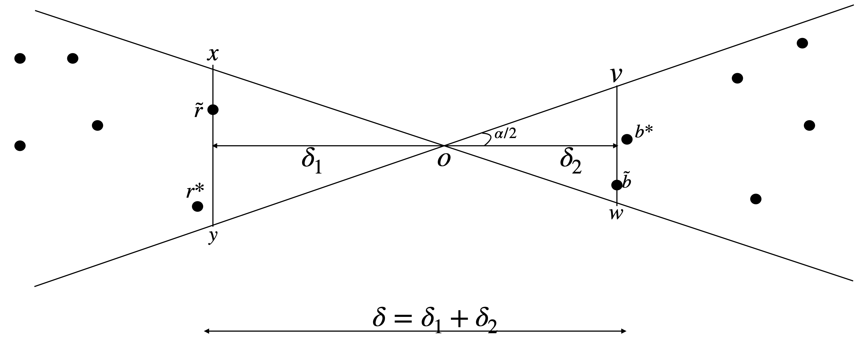
For this, we will first make the simplifying assumption that no two points in $P$ share a coordinate in any of the bases $(e_j,e_{j+1})$, and that no two points have the same projection in any of the directions $d_j$, for any $0\le j\le 19$. It is not hard to remove this assumption by randomly perturbing the basis vectors above, as the argument does not hinge on them being uniformly distributed; it just relies on all angles being at most ${\alpha }_0$ and on the union of the double wedges covering ${ℝ}^2$.

Refer to Figure 2. Since $\tilde{r}$ is the red point with maximum projection on the direction $d$ (without loss of generality considered here to be horizontal), $r^{\ast }$ must lie to the left of the line segment $xy$. Similarly $b^{\ast }$ must lie to the right of the line segment $vw$. Let the horizontal distance between the projections of $\tilde{r}$ and $\tilde{b}$ be $\delta$, and we break this up into ${\delta }_1+{\delta }_2$, with ${\delta }_1$ being the portion of it in the left wedge and ${\delta }_2$ being the portion of it in the right wedge. Also note that since the direction $d$ is the bisector of the wedge, the interior angles between the direction of the $x$-axis and either of the lines defining the wedge, are $\alpha /2$.

We first prove (c). Since $\tilde{r}$ is constrained to lie on the line $xy$ and $\tilde{b}$ on $vw$, the maximum distance between them is obtained when $\tilde{r}=x$ and $\tilde{b}=w$. This distance is ${\delta }_1\sec (\alpha /2)+{\delta }_2\sec (\alpha /2)=\delta \sec (\alpha /2)$. Thus $d(\tilde{r},\tilde{b})\le \delta \sec (\alpha /2)$. On the other hand, $d(r^{\ast },b^{\ast })$ is at least $\delta$, as otherwise either $r^{\ast }$ is to the right of $xy$ or $b^{\ast }$ is to the left of $vw$, contradicting that $\tilde{r}$ and $\tilde{b}$ were the points with the extremal projections. Therefore, $\frac{d(\tilde{r},\tilde{b})}{d(r^{\ast },b^{\ast })}\le \frac{\delta \sec (\alpha /2)}{\delta }=\sec (\alpha /2)$. Recall that $\alpha =\pi /10$, plus some minor perturbation to make the above assumption hold, if necessary, which proves (c).

Next we prove (a). Assume the wedge is centered at the origin, so that $r^{\ast }$ has x-coordinate equal to $-({\delta }_1+{ϵ}_1)$ and $b^{\ast }$ has $x$-coordinate ${\delta }_2+{ϵ}_2$, for some ${ϵ}_1>0$, ${ϵ}_2>0$. We claim that ${ϵ}_1\le \delta (\sec (\alpha /2)-1)$. To see this, assume the contrary. Then the distance $d(r^{\ast },b^{\ast })$ is at least ${\delta }_1+{\delta }_2+{ϵ}_1+{ϵ}_2$, which is larger than $\delta +{ϵ}_1$, and therefore by the assumption is larger than $\delta \sec (\alpha /2)$. However, we just showed that $d(\tilde{r},\tilde{b})\le \delta \sec (\alpha /2)$, and this contradicts that $(r^{\ast },b^{\ast })$ is the exact solution to the BCP instance.

Next, let us assume that the $y$-coordinate of $r^{\ast }$ is $t^{\ast }$ and that of $\tilde{r}$ is $\tilde{t}$. Thus $r^{\ast }=(-{\delta }_1-{ϵ}_1,t^{\ast })$ and $\tilde{r}=(-{\delta }_1,\tilde{t})$. Note that $|\tilde{t}|\le {\delta }_1\tan (\alpha /2)$, since that is the $y$-coordinate of $x$ and $\tilde{r}$ must lie on $xy$. Similarly, we get that $|t^{\ast }|\le ({\delta }_1+{ϵ}_1)\tan (\alpha /2)$, since $r^{\ast }$ is constrained to lie in the left wedge.

We obtain that the distance $d(\tilde{r},r^{\ast })\le {ϵ}_1+|\tilde{t}|+|t^{\ast }|$. Using the bounds on ${ϵ}_1$, $|\tilde{t}|$ and $|t^{\ast }|$, this is at least

In the above we have used that ${\delta }_1\le \delta$, , and that for $\alpha =\pi /10$, . Finally, we use that $d(r^{\ast },b^{\ast })>\delta$. A similar argument can be used to prove that and this finishes the proof of (a).

Finally, we prove (b). Our proof is inspired by an argument by Callahan [7]. Consider any pair of points $p,q\in P$. We want to show that there is a path between them in $G$. Let $T$ denote the Euclidean MST. We will show that $G$ contains such a path by using induction on the length of the longest edge in the path connecting $p$ to $q$ in $T$. Let $e$ be the longest edge in the path in $T$ connecting $p$ to $q$, and because $e$ is an MST edge, it must be of the type $e=(r^{\ast },b^{\ast })$ for some bichromatic closest pair in one of the instances. Assume that $r^{\ast }$ is encountered first on this path when walking from $p$ to $q$. This edge $e=(r^{\ast },b^{\ast })$ is replaced by the approximate edge $(\tilde{r},\tilde{b})$ in $G$. We claim that there is a path connecting $p$ to $\tilde{r}$ in $T$ that only uses edges cheaper than $e$ – one goes from $p$ to $r^{\ast }$ in $T$ using edges cheaper than $e$, and by (a), . Applying the induction hypothesis we get that there is such a path from $p$ to $\tilde{r}$ in $G$ too. Similarly there is path in $G$ from $q$ to $\tilde{b}$ such that all edges have length at most $|e|$. Since the edge $(\tilde{r},\tilde{b})$ is in $G$, this implies that there is path from $p$ to $q$ in $G$, and hence $G$ is connected. This finishes the proof of correctness and the approximation guarantee of our algorithm, summarized as follows. $◀$

Several open problems emerged as a result of this research and at the suggestion of the anonymous referees. Is it possible to solve Convex Hull in $O(\log n\log h)$ fragility, where $h$ is the number of hull vertices? Does there exist an algorithm to compute a Voronoi Diagram or Delaunay Triangulation in sublinear fragility? Is it possible to obtain a $\mathrm{\Omega }({\log }^{2}n)$ lower bound on any problem addressed in this paper?

References

- [1] Peyman Afshani, Rolf Fagerberg, David Hammer, Riko Jacob, Irina Kostitsyna, Ulrich Meyer, Manuel Penschuck, and Nodari Sitchinava. Fragile Complexity of Comparison-Based Algorithms. In 27th Annual European Symposium on Algorithms (ESA 2019), volume 144 of Leibniz International Proceedings in Informatics (LIPIcs), pages 2:1–2:19, Dagstuhl, Germany, 2019. Schloss Dagstuhl – Leibniz-Zentrum für Informatik. doi:10.4230/LIPIcs.ESA.2019.2.
- [2] Pankaj K Agarwal, Herbert Edelsbrunner, Otfried Schwarzkopf, and Emo Welzl. Euclidean minimum spanning trees and bichromatic closest pairs. In Proceedings of the Sixth Annual Symposium on Computational Geometry, pages 203–210, 1990. doi:10.1145/98524.98567.
- [3] Miklós Ajtai, János Komlós, and Endre Szemerédi. An O(n log n) sorting network. In Proceedings of the 15th Annual ACM Symposium on Theory of Computing, 25-27 April, 1983, Boston, Massachusetts, USA, pages 1–9. ACM, 1983. doi:10.1145/800061.808726.
- [4] Michael Ben-Or. Lower bounds for algebraic computation trees. In Proceedings of the Fifteenth Annual ACM Symposium on Theory of Computing, pages 80–86, 1983.
- [5] Prosenjit Bose, Pilar Cano, Rolf Fagerberg, John Iacono, Riko Jacob, and Stefan Langerman. Fragile complexity of adaptive algorithms. In International Conference on Algorithms and Complexity, pages 144–157. Springer, 2021. doi:10.1007/978-3-030-75242-2_10.
- [6] Prosenjit Bose, Anil Maheshwari, Pat Morin, Jason Morrison, Michiel Smid, and Jan Vahrenhold. Space-efficient geometric divide-and-conquer algorithms. Computational Geometry, 37(3):209–227, 2007. doi:10.1016/J.COMGEO.2006.03.006.
- [7] Paul B Callahan. Dealing with higher dimensions: the well-separated pair decomposition and its applications. The Johns Hopkins University, 1995.
- [8] Thomas H Cormen, Charles E Leiserson, Ronald L Rivest, and Clifford Stein. Introduction to algorithms. MIT press, 2022.
- [9] Karthik C.S. and Pasin Manurangsi. On closest pair in Euclidean metric: Monochromatic is as hard as bichromatic. Combinatorica, 40(4):539–573, 2020. doi:10.1007/S00493-019-4113-1.
- [10] Mark De Berg, Otfried Cheong, Marc Van Kreveld, and Mark Overmars. Computational Geometry: Algorithms and Applications. Springer, 2008.
- [11] Jeff Erickson. Lecture notes for cs 497: Concrete models of computation, spring 2003.
- [12] Ronald L. Graham. An efficient algorithm for determining the convex hull of a finite planar set. Info. Proc. Lett., 1:132–133, 1972. doi:10.1016/0020-0190(72)90045-2.
- [13] Ray A Jarvis. On the identification of the convex hull of a finite set of points in the plane. Information Processing Letters, 2(1):18–21, 1973. doi:10.1016/0020-0190(73)90020-3.
- [14] Rajesh Jayaram, Vahab Mirrokni, Shyam Narayanan, and Peilin Zhong. Massively parallel algorithms for high-dimensional euclidean minimum spanning tree. In Proceedings of the 2024 Annual ACM-SIAM Symposium on Discrete Algorithms (SODA), pages 3960–3996. SIAM, 2024. doi:10.1137/1.9781611977912.139.
- [15] David G Kirkpatrick and Raimund Seidel. Output-size sensitive algorithms for finding maximal vectors. In Proceedings of the First Annual Symposium on Computational Geometry, pages 89–96, 1985. doi:10.1145/323233.323246.
- [16] David G Kirkpatrick and Raimund Seidel. The ultimate planar convex hull algorithm? SIAM Journal on Computing, 15(1):287–299, 1986. doi:10.1137/0215021.
- [17] H. T. Kung, Fabrizio Luccio, and Franco P. Preparata. On finding the maxima of a set of vectors. J. ACM, 22(4):469–476, 1975. doi:10.1145/321906.321910.
- [18] Mark H Overmars and Jan Van Leeuwen. Maintenance of configurations in the plane. Journal of computer and System Sciences, 23(2):166–204, 1981. doi:10.1016/0022-0000(81)90012-X.
- [19] Franco P. Preparata and Se June Hong. Convex hulls of finite sets of points in two and three dimensions. Communications of the ACM, 20(2):87–93, 1977. doi:10.1145/359423.359430.
- [20] Franco P Preparata and Michael I Shamos. Computational Geometry: An Introduction. Springer Science & Business Media, 2012.
- [21] Michael Ian Shamos and Dan Hoey. Closest-point problems. In 16th Annual Symposium on Foundations of Computer Science (sfcs 1975), pages 151–162. IEEE, 1975. doi:10.1109/SFCS.1975.8.
- [22] Andrew Chi-Chih Yao. On constructing minimum spanning trees in k-dimensional spaces and related problems. SIAM Journal on Computing, 11(4):721–736, 1982. doi:10.1137/0211059.