Global Polyline Simplification Under the Fréchet Distance: Theory and Practice

Abstract
Given an input polyline with vertices, the global polyline simplification problem seeks a simplified polyline with the minimum number of vertices whose distance to the original polyline does not exceed a given bound. For the vertex-restricted variant, where the simplified polyline is required to be a subsequence of the input vertices, an algorithm with a running time of was presented in previous work, using the Fréchet distance as the polyline similarity measure. A closely related variant is the local polyline simplification problem, in which the distance bound is required to hold for every individual shortcut segment replacing a sub-polyline. This condition implies that any locally valid simplification is also globally valid, whereas the converse does not hold. As a consequence, globally optimal simplifications may use substantially fewer vertices than locally optimal ones. Indeed, in previous work, instances were constructed in which the optimal global simplification is smaller by a constant factor. On the algorithmic side, optimal local simplifications can be computed significantly faster, namely in under the Fréchet distance, and efficient heuristics are also available. This raises the question of which problem variant is more suitable for practical application.
In this paper, we first show that there exist instances for which the optimal solution sizes of global and local polyline simplification differ by a factor in , substantially strengthening the previously known constant-factor separation. We then present the first practical implementations of existing algorithms for global polyline simplification and experimentally evaluate their performance. To this end, we introduce several engineering techniques that considerably accelerate these algorithms. Moreover, we develop an implicit Fréchet framework that allows many Fréchet-related problems to be addressed in a weaker computational model. Within this framework, explicit geometric computations can be reduced to simple comparisons, resulting in significantly more robust implementations. Somewhat surprisingly, our experimental results reveal that, despite the large worst-case gap established by our theoretical result, the difference in solution size between optimal global and local simplifications is negligible in practice. Motivated by this observation, we propose a heuristic for global polyline simplification that is guaranteed to produce solutions of size equal to or smaller than the optimal local simplification. On a benchmark consisting of one million polylines, the heuristic yields suboptimal results on only eight while being significantly faster than the optimal algorithms.
Keywords and phrases:
Polyline Simplification, Shortcut Graph, Fréchet DistanceCopyright and License:
![[Uncaptioned image]](x1.png) © Christian Abdullahad and Sabine Storandt; licensed under Creative Commons License CC-BY 4.0
© Christian Abdullahad and Sabine Storandt; licensed under Creative Commons License CC-BY 4.0
2012 ACM Subject Classification:
Theory of computation Computational geometry ; Theory of computation Design and analysis of algorithmsEditors:
Martin Aumüller and Irene FinocchiSeries and Publisher:
 Leibniz International Proceedings in Informatics, Schloss Dagstuhl – Leibniz-Zentrum für Informatik
1 Introduction
Polyline simplification is the process of algorithmically reducing the number of vertices of a polyline while preserving its general shape. Applications include the simplification of map contours in geographic information systems [7], noise reduction in movement trajectories [13, 14], and compressing linear data [15, 12].
There are different flavours of polyline simplification, which differ by the constraints the simplified polyline must obey and how the shape similarity to the input polyline is measured. In this paper, we focus on vertex-restricted simplifications, where the simplified polyline must be a subsequence of the original polyline vertices. The simplification problem then asks for the simplified polyline of smallest size for which the distance to the original polyline does not exceed a given error bound . Different distance measures are used in the literature, with the most common ones being the Hausdorff and the Fréchet distance. These distance measures can be applied both locally and globally. In the local version, the error bound must be obeyed for each shortcut between consecutive points in the simplified polyline and the original sub-polyline it replaces. In the global version, the error bound simply needs to be obeyed for the original and the simplified polyline as a whole. The local version has been studied for a long time [11]. Optimal local simplifications in can be computed in time under the Hausdorff distance [5] and in under the Fréchet distance [17], and practical implementations are available as well. In contrast, the global variant has been studied only recently [19, 18]. Somewhat surprisingly, global simplification under the Hausdorff distance turned out to be NP-hard. For the Fréchet distance, -time algorithms are known [4, 18], but they have not been experimentally evaluated so far.
By definition, any local simplification respecting is also a feasible global simplification for the same error bound, but the converse is not true. Therefore, global simplifications might be smaller than local ones, but the price to pay is a substantially higher theoretical running time. The goal of this paper is to compare the practical applicability of local and global simplification. In particular, we are interested in the following two core questions:
-
Is it possible to implement known exact algorithms for global polyline simplification such that they scale to large inputs despite their (super)cubic theoretical running times?
-
How much do global and local simplification sizes differ in practice?
To answer these questions, we provide novel theoretical insights, present several engineering techniques for global simplification, and conduct a thorough experimental evaluation on synthetic and real data sets.
1.1 Related Work
Local simplification has been extensively studied. Under the Fréchet distance, the Imai-Iri algorithm computes an optimal solution in by constructing a so-called shortcut graph in which the shortest path coincides with the smallest feasible simplification. The efficiency of the graph construction step was improved in [17], resulting in a running time of and significantly faster computation in practice. Furthermore, heuristics are commonly applied, such as the Douglas-Peucker algorithm with a running time of (and no quality guarantee) [7] and the approximation algorithm by Agarwal et al. [1], which runs in and guarantees that the computed simplification size does not exceed the optimal one for a parameter .
The concept of global simplification was touched upon in [1] and [3], but only in the context of weak simplification or when using the discrete Fréchet distance as the error measure. The systematic study of vertex-restricted global polyline simplification was initiated by van Kreveld et al. [19]. They show that neither the Douglas-Peucker nor the Imai-Iri algorithm produce optimal solutions for this problem variant, and present an exact algorithm with a running time in , where denotes the output size. This running time was later reduced to by Bringmann and Chaudhury [4] as well as van de Kerkhof, Kostitsyna, Löffler, Mirzanezhad, and Wenk [18]. In [4], a conditional lower bound is presented, making the existence of subcubic algorithms for global simplification in high dimensions unlikely.
The one dimensional case is the only case where subcubic algorithms are known for the Fréchet setting, in fact local and global Fréchet simplifications have the same size and can be computed in linear time. Although this result was established by Driemel et al. [9], its significance appears to have been overlooked in subsequent literature111For example, [18] rediscovered the linear time algorithm but only for the curve-restricted setting; they do not mention it for the other settings., likely because the original authors framed it within a non-optimality claim. In the setting where the start and end vertex are required to be in the simplification, their finding is, in fact, optimal.
Their algorithm can be stated simply: Include the first polyline vertex in the simplification and traverse all vertices until the first outside of is found and go towards the direction where leaves this range; for simplicity, assume that we go right. Maintain the right-most vertex found. If for the current vertex , append to the simplification and reverse the direction. A similar algorithm also works for the local Hausdorff setting with the small modification that we change direction when a vertex left of is found (or right of when going left), where is the previously found vertex in the simplification. The global Hausdorff setting is trivial since we only need to include the start and end vertices as well as potentially the left-most and right-most vertices. If the left-most or right-most vertex is within of the start or end, or between the two, we do not need to include them; otherwise, we do.
1.2 Contribution
First, we investigate the maximum possible difference in size between optimal global and local simplification. Previous work established that there can be a constant-factor gap between them [18]. We significantly strengthen this separation by constructing a class of polylines for which optimal global and local simplification differ by a factor in . Thus, our bound is asymptotically tight, rules out local simplification algorithms as approximation algorithms for global simplification, and illustrates the significant potential of simplification size reduction when using global simplification.
To compare the simplification sizes and running times of global and local simplification algorithms in practice, we provide the first implementations222The implementation as well as data is publicly available at https://github.com/Ingemisco/Global-Polyline-Simplification-under-the-Frechet-Distance-Theory-and-Practice of the exact algorithms for global simplification by Bringmann and Chaudhury [4] and by van Kreveld et al. [19]. We describe several engineering techniques to significantly reduce their running times and space consumption. Furthermore, we address the fact that these algorithms rely on geometric computations prone to numerical issues. We present an implicit Fréchet framework that abstracts explicit equation solving into a small set of decision problems. We show that all algorithms discussed here, as well as many related algorithms, can be rewritten using these decision problems. This allows us to assume a weaker model of computation. In the Euclidean case, this allows us to avoid square root computations, thus operating within the regular RAM model of computation. Using this framework in our implementation yields a slower but more robust implementation. Despite the theoretical cubic running time, our experimental evaluation demonstrates that optimal solutions for polylines with hundreds of vertices can be computed in seconds. This allows us to evaluate the difference between global and local simplification sizes on practical instances for the first time. Interestingly, instances on which they do not produce the same solution size are rare and the maximum observed gap is tiny (especially compared to our theoretical worst-case gap example). Finally, using the classic Imai-Iri algorithm as a basis, we derive a global simplification algorithm that is equivalent to the one by the authors of [18] but presented in a more intuitive way. We then show how to modify this algorithm into a simple heuristic that is guaranteed to find a solution at least as good as the local optimal one. In practice, the heuristic outperforms the exact algorithms while yielding optimal solutions on almost all tested instances.
2 Preliminaries
A -dimensional polyline of length is a sequence of points (called vertices) in -dimensional space. We interpret a polyline as a continuous functions with for and . We denote by the sub-polyline . For two points , the polyline of length 1 is also written as and is called line segment or shortcut.
Definition 1 (Minkowski Distance).
Let . The -Minkowski distance between two points is defined as . The special case of is called the Manhattan distance, is the Euclidean distance. We also set which is the Chebyshev distance.
Definition 2 (Fréchet Distance).
Given a distance between points, the Fréchet distance between polylines and of lengths and , respectively, is
where and are continuous non-decreasing functions with , , and .
Definition 3 (Polyline Simplification).
Fix a distance measure between polylines. Given a polyline of length and . A subsequence of of length , with , is called
-
a global simplification of if .
-
a local simplification of if for all .
If is minimal, we call the simplifications minimal global simplification and minimal local simplification, respectively.
These are also called vertex-restricted simplifications because the simplification can only select among the polyline vertices. In the remainder of the paper, unless stated otherwise, we are concerned with vertex-restricted polyline simplification in dimensions under the Fréchet distance with the Euclidean norm.
3 Global vs. Local Simplification Size
Van Kreveld et al. [19] provided an example polyline with ten vertices for which, under a carefully chosen Fréchet distance bound , the optimal local simplification contains all input vertices, while the optimal global simplification contains only eight. This polyline gadget can be concatenated to produce a polyline of arbitrary length for which the local simplification size is times larger than the global one. This left open the question333Similar results are already known but to our knowledge unpublished. of whether the local simplification always provides a constant-factor approximation for the global one.
We now answer this question negatively.
Theorem 4.
For any , there exists a polyline with vertices for which the optimal local simplification is larger than the optimal global simplification by a factor in .
Proof.
We construct a polyline for which the optimal local simplification contains all original vertices, while the optimal global simplification contains only a constant number. The polyline is illustrated in Figure 1.
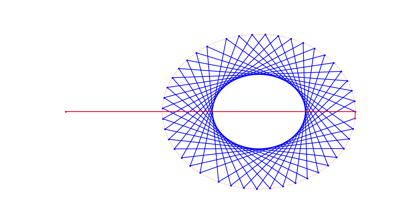
To construct such a polyline of length , we choose the first two vertices such that the shortcut between them passes through the centre and the second vertex lies on the circle of radius . We then choose444One way to obtain a valid is as follows: with vertices approximately rotations around the circle are needed for . Shrink minimally such that the condition on the endpoint is met. At most one full rotation from the will be removed. Distributed over all edges might be subtracted from which yields a valid for large enough. Similar constructions can be found manually for small . an irrational number and place all remaining vertices on the circle such that each subsequent vertex forms an angle of with the previous vertex and the centre. The exact value of must be chosen so that . The irrationality of guarantees that no other shortcut passes through the centre. In the figure, the red dotted circle represents the -neighbourhood, and the global simplification is shown in red. The optimal global simplification requires only the vertices , because the shortcut passes through the centre of the circle, from which all points are within distance . However, no local shortcut that skips at least one vertex exists because, by construction, for any such shortcut there is at least one skipped vertex whose distance to the shortcut exceeds . Thus, the local simplification requires all vertices.
4 Algorithms for Global Simplification
In this section, we first briefly recap the exact algorithms for global simplification presented in [19] and [4], which have running times in and , respectively, where is the number of vertices in the input polyline and denotes the output size. For more details, we refer to the original papers. Both algorithms use dynamic programming to store and compute all information necessary to construct the simplification. We also describe several engineering techniques to boost their practical performance. Subsequently, we propose a novel heuristic for global simplification. This heuristic is based on a reinterpretation of the algorithm by the authors of [18] and leverages the Imai-Iri algorithm, which was originally introduced for local simplification.
4.1 Exact Algorithms
To describe the exact algorithms concisely, we introduce the following notation.
Definition 5.
Fix and a distance function . Given a line segment and a point , we define and . If the set is empty, we define both functions to be .
The algorithm by van Kreveld et al. [19] uses dynamic programming with a three-dimensional table . The value stored in is the smallest for which there exists a partial simplification of with exactly shortcuts such that . If no such exists, we set . If for some , a simplification can be extracted from because and lies on the last line segment. The smallest such is denoted by . For , the entries are computed trivially. For , each layer is computed from the previous one. To compute , we iterate over all with and , and determine the minimum for which (if such a exists), where . To test whether this Fréchet distance is within and obtain the respective , a modified555We do not need to explicitly compute the Fréchet distance allowing a simpler algorithm. version of the algorithm from Alt and Godau [2] can be used which runs in . Thus, the minimization can be performed in cubic time per cell entry, leading to a total runtime of . For better practical runtimes, we introduce the following trivial optimizations:
-
Reachability: If no point on lies within of , then for all , and no minimization is needed.
-
Local Minimality: When computing , the minimization can be stopped early if the computed minimum equals .
-
Global Minimality: If , this value can be copied to .
The correctness of the first optimization is straight-forward. For the local and global minimality optimizations, correctness follows from comparing with the lower bound for . Finally, we note that the computations for each layer can be parallelized because they depend only on the previous layer.
To reduce the running time to , Bringmann and Chaudhury split the minimization for computing into two cases: and . The value of is then the minimum of the values computed for these two cases. The case can be solved in constant time per cell entry by maintaining a minimum. The case is more complicated; they introduce the cell reachability problem to compute minimal cell entries in linear time, yielding constant amortized time per cell entry. Their modifications restructure the algorithm because of the more complex data flow. The outermost loop is over instead of , resulting in total runtime of rather than the expected 666Revisiting their conditional lower bound proof rules out algorithms for any and , as the simplification in their reduction has constant size..
The more complicated data flow prevents the application of the optimizations discussed above for the van Kreveld et al. algorithm. Furthermore, parallelization is difficult to apply in this restructured algorithm. Thus, especially for small polylines, the van Kreveld et al. algorithm may be faster in practice.
4.2 A Heuristic for Global Simplification
Next, we discuss how to adapt the classic Imai-Iri algorithm, originally proposed for local simplification, to the global case. This yields an algorithm equivalent to the one from the authors of [18] but provides a fresh perspective. We argue that this algorithm achieves cubic (and possibly subcubic) runtime for certain classes of polylines and use this observation to formulate a new heuristic that has the potential for improved running time in practice.
4.2.1 Local and Global Imai-Iri
The Imai-Iri algorithm [11] for local simplification relies on the construction of a shortcut graph whose vertices correspond to the polyline vertices, with directed edges for if is a local shortcut, i.e., . The simplification is the shortest path from to in the shortcut graph.
We first derive the notion of a global shortcut graph (GSG) for global simplification. Unlike in the local setting, storing only whether a valid shortcut exists is insufficient because each shortcut may correspond to multiple sub-polylines with . For a shortcut , a sub-polyline is called -admissible if . For brevity, we denote sub-polylines by the pair . We need to compute and store all -admissible sub-polylines for each shortcut . Admissibility depends on the points near the endpoints of . For the rest of this section are real-valued points of the polyline and are vertices.
Definition 6.
For a vertex , the non-empty set is the disjoint union of at most closed intervals (at most one per line segment). We denote the ordered list of these intervals by . Intervals may contain multiple line segments, and for each there is a unique interval in containing . Moreover, if is -admissible, then and .
Lemma 7.
Let be a shortcut and be -admissible.
-
1.
If with , then is -admissible.
-
2.
If with , then is -admissible.
-
3.
If , and , then is -admissible.
-
4.
If , and , then is -admissible.
Proof.
For all of these properties note that each cell in the free space diagram is convex. By the preconditions there is a path through the cell which can be adapted to the desired path. Refer to Figure 2.
By Lemma 7, -admissibility is a property between intervals and . We say that is -admissible if is -admissible for some and . Note that we still cannot go backward so any such is -admissible only if . Further, for a fixed , the admissible intervals are all consecutive in , meaning that no inadmissible interval in is between two admissible ones, allowing to store all of them as one meta-interval.
Definition 8 (Global Shortcut Graph).
The global shortcut graph of a polyline of length is the directed graph where and . Additionally, for each , we store the ordered list . For each shortcut , we store the admissible sub-polylines as an ordered list of pairs of intervals . Each is an interval from , and the corresponding is the smallest closed interval containing all intervals for which is admissible.
We denote this ordered list of pairs of intervals for the shortcut by and call its elements mappings.
For an example, refer to Figure 3. This shows all the data for the shortcut . Paths that witness admissibility in the free space diagram are shown in black.
With this data structure, testing whether a sub-polyline is -admissible is simple: we check that , , , and for some777The pair is unique since is contained in at most one such interval . mapping . The interval data per vertex can be computed in linear time per vertex, yielding total quadratic runtime. Computing the mappings can be done in worst-case linear time per edge using a procedure similar to the cell reachability algorithm from [4] (the free space diagram in Figure 3 has almost identical structure to cell reachability).
For each shortcut maintain an initially empty queue888Bringmann and Chaudhury maintain an ordered list; a queue suffices. of active intervals while traversing the polyline and intervals in . If the queue is empty, skip in the polyline to the next interval in . Otherwise, process the vertices like in cell reachability. If a new interval in starts, push it to the front of the queue with a value of . Between two consecutive cells there are passage (in Figure 3 shown in green) that restrict how paths are allowed to pass to the next cell. When transitioning to the next cell, remove all intervals whose assigned value is above the passage from the back of the queue and merge all intervals whose value is below the passage at the front of the queue and assign as new value the start of the passage.
Thus, the graph can be computed in cubic time, dominated by the computation of the mappings. In practice, computing the mappings can be accelerated as follows:
-
1.
If the queue is empty, skip to the cell corresponding to the start of the next interval in .
-
2.
When inserting an interval into an empty queue, skip all cells until the end of the interval (accounting for intervals in that intersect it).
-
3.
If no further interval exists in , stop.
With these optimizations, the construction time can be quadratic for favourable polylines and values of . Having computed all data, we traverse the graph to construct the simplification. This traversal is more complicated than in the original Imai-Iri algorithm. For each vertex , we compute all sub-polylines for which there exists a partial simplification using the vertices (starting at and ending at ) such that . These sub-polylines are represented as intervals. For , we store the interval in and associate it with an empty simplification. For a vertex , we iterate over all previous vertices and attempt to append the shortcut . This involves traversing the reachable data for and the mappings in a merge-like procedure. Finally, we consider intervals of the form and select the smallest simplification found.
The runtime depends on the amount of data that must be considered per vertex. For each vertex and interval , at most different simplifications (one per possible length) may be needed. Specifically, if any point in is reachable with a partial simplification, then all points to the right in are reachable with the same simplification. Since we need only minimal partial simplifications, this data can be sorted in decreasing order of simplification size. Propagation per vertex can be done in quadratic time per shortcut, leading to cubic time per vertex and a total quartic time. Intervals can be split in advance to allocate space, or lazily as needed. Lazy splitting occurs only for mappings of the form with , because only the subinterval is reachable (we cannot traverse backward). If such negative mappings (for an example, the mapping in Figure 2 is a negative mapping) are rare, the algorithm runs in cubic time, or even in quadratic time if the number of intervals is small. This is an advantage over the Bringmann and Chaudhury algorithm, whose running time is . Without negative mappings, only one entry per interval is needed, resulting in quadratic space usage999This requires computing edge data in the GSG only when needed, an optimization also applicable to the local Imai-Iri algorithm..
4.2.2 Heuristic
The algorithm described above produces the optimal simplification in time. However, for GSGs without negative mappings, the running time is cubic or better. Not all polylines produce such GSGs. Therefore, we propose the following transformations which turn the exact algorithm into a heuristic:
-
For each , split the unique interval containing into and .
-
For each negative mapping , shrink the interval to in .
The second step modifies negative mappings but may also remove some mappings because the shrunken interval may no longer correspond to a valid mapping. To ensure that a simplification is always found, we use the first step. This guarantees that all local shortcuts remain in the graph because interval always contains (we only shrink from the left). Thus, the computed simplification is at least as good as the optimal local simplification and is suboptimal only if the interval structure is very intricate. For example, for the polyline constructed in Figure 1, the heuristic yields the optimal global simplification, demonstrating that it can produce significantly smaller simplifications than any local simplification algorithm.
5 Implicit Fréchet Framework
Typically, the Fréchet distance is studied in the real RAM model, where equations for and (see Definition 5) can be solved with arbitrary precision in constant time. This simplifies runtime analysis, but algorithms require sufficiently accurate approximations. For the Manhattan and Chebyshev distance, these equations use only addition, subtraction, and multiplication, so the regular RAM suffices. The Euclidean case, however, requires square roots for quadratic equations. Higher Minkowski distances lack closed-form solutions due to the Abel-Ruffini theorem. In the implicit Fréchet framework, we replace these explicit solution computations with new primitives. The key insight is that only comparisons are needed. Instead of explicit solutions, we provide solvers for the comparisons.
These techniques to avoid square roots in the Euclidean case are already known in the field of computational geometry. Our primitives reduce to inequalities of the form which can be decided without the use of square roots (e.g., refer to [6]). Here, we present a structured approach to apply such techniques to Fréchet-based problems, especially polyline simplification. We chose to include this discussion since we studied and implemented all relevant primitives for polyline simplification and no previous global simplification algorithms were implemented.
For any fixed , we define three decision problems:
Definition 9.
Let be a line segment and be points.
-
reaches (denoted ) if ; equivalently, a point on is within of .
-
If , then proceeds to on (denoted ) if and .
-
If , then waits for on (denoted ) if and .
These relations and can also be viewed in the dog-walking intuition that is often used when it comes to the Fréchet distance. The dog acts as the restriction while the path that you travel on is the line segment . If the dog runs away, it forces you to move () to a new position. The dog may also walk somewhere in your surrounding, in which case you can just wait ().
Note that can be implemented using because if and only if . We include it for intuition, for ease of solution, and because it is sometimes necessary. Examples are shown in Figure 4.
| Explicit operation | Implicit operation | Comment |
|---|---|---|
| replaces solution | ||
| are solutions on , | ||
| and are restrictions | ||
| if then else | are solutions on | |
| and are restrictions | ||
| if then else | are solutions on | |
| and are restrictions | ||
| is the restriction for | ||
| exists |
Many Fréchet algorithms only track earliest reachable points, which can only proceed or wait but never go backward. This behaviour is modeled by and . Instead of an explicit earliest point, we store the vertex whose solution causes it, called a restriction.
Table 1 summarizes how to translate various explicit computations with implicit ones. This includes all operations necessary for the described exact algorithms for global simplification. We use for variable assignment and for the wait relation.
To solve these relations in Euclidean space, we write the explicit solutions for and compare them directly. This results in inequalities of the form since are solutions to quadratic equations. How to decide such inequalities is already well-established.
5.1 Applying the decision problems
We demonstrate the conversion using the Alt and Godau algorithm [2], which decides whether . For simplicity, we assume is a line segment (as in the minimization step of van Kreveld et al.’s algorithm). The general case and other algorithms convert similarly. Let be the length of . In the explicit variant, the value is computed and stored dynamically. In our implicit variant, we instead store restrictions (vertex indices). First, test whether and . For general Minkowski distances, this test may involve higher-order roots, but it can be performed without them by raising both sides to the appropriate power. The algorithm tracks the earliest reachable point on while traversing . We replace these points with restrictions. The initial restriction is ; note that because . Let be the current restriction. When processing vertex , test whether . If so, update . If keep . Otherwise, report .
In Listing 1, we show both the explicit and implicit version of the algorithm from Alt and Godau as used in the algorithm from van Kreveld et al. This version takes as additional input a parameter and outputs a or as mentioned in Section 4.1.
5.2 Semiexplicit Algorithms
The semiexplicit approach provides another method for implementing Euclidean Fréchet algorithms without square roots. It combines characteristics of both explicit and implicit algorithms. In the Euclidean case, the decision problems require only comparisons of the form , which can be decided without evaluating square roots. The idea of semiexplicit Euclidean variants is to define data types that store such and and define appropriate comparison operators between them. In programming languages that support parametric polymorphism, the code for semiexplicit and explicit variants can be identical. For example, in C++, we can use templates and operator overloading to implement algorithms. By instantiating the templates with different data types, we obtain both explicit and semiexplicit variants. This makes it straightforward to implement both variants while retaining the benefit of avoiding square root computations.
6 Experimental Results
The goal of this section is to compare the running times and output sizes of local and global simplification algorithms. We implemented the Imai-Iri algorithm to obtain optimal local simplifications, the two discussed exact algorithms for global simplification, and our novel heuristic. We refer to the algorithm by van Kreveld et al. as KLW and the algorithm by Bringmann and Chaudhury as the BC algorithm. All algorithms were implemented to work with the Manhattan, Chebyshev, and Euclidean norms. For the Euclidean norm, we implemented explicit, semiexplicit, and implicit variants. All algorithms were implemented in C++ and compiled with GCC using optimization flags -O3 and -flto. The variants of the KLW algorithm were parallelized using OpenMP with dynamic scheduling and a chunk size 32. All experiments were run on a machine with an AMD Ryzen 5 7520U CPU (4.38 GHz, 8 cores) running Arch Linux.
6.1 Benchmark Data Sets
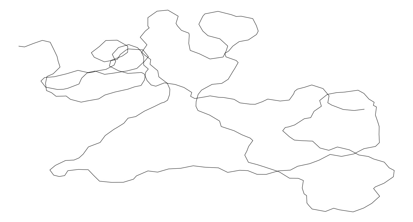
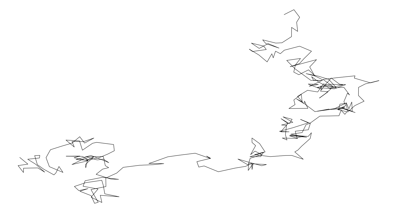
We use synthetic and real-world data in our experiments. Synthetic polylines were generated using a custom method that takes as input the vertex count, minimum and maximum segment lengths and , and maximum deviation angle between consecutive line segments (e.g., means no restriction, yields a straight line). Smaller values of produce smoother polylines. Deviation angles are drawn uniformly from . Segment lengths are generated via inverse transform sampling using the formula , where and is the dimension. This ensures that the vertices are distributed uniformly in the annulus section defined by , and . We set and , respectively. We created two benchmarks sets; example instances from each are shown in Figure 5:
-
well-behaved (w) polylines with a maximum angle of , and
-
non-well-behaved (n) polylines with a maximum angle of .
Unless stated otherwise, we use in all experiments. We use this because for our choices of parameters for data generation it often yielded interesting simplifications. Smaller tend to use almost all vertices and large often use a constant number of vertices. The choices for for the data generation were arbitrary.
Our real-world data consists of 100 openly available GPS traces101010Data from https://www.openstreetmap.org/traces/ uploaded December 29–30 and January 9, converted from GPX. with vertex counts between 100 and 800. We used the longitude and latitude coordinates, translated each trace to start at the origin, and scaled them so that the median segment length is 10. Translation does not affect the simplifications, and scaling only changes the effective value of .
6.2 Runtimes
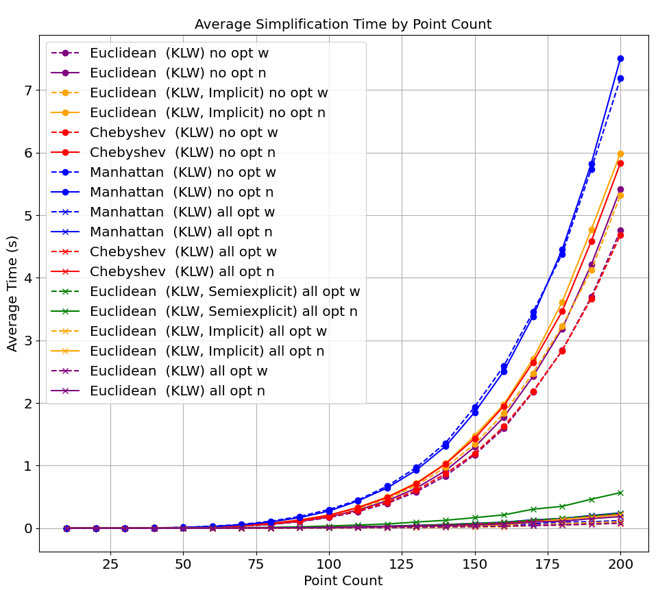
First, we compare the effect of our three proposed optimizations on the runtime of the KLW algorithm (Figure 7). We observe that they significantly reduce the running time for all norms and algorithm configurations. For example, in the implicit Euclidean setting, the runtime decreases from about 6.0 seconds (non-well-behaved) and 5.4 seconds (well-behaved) to less than 300 milliseconds for both.
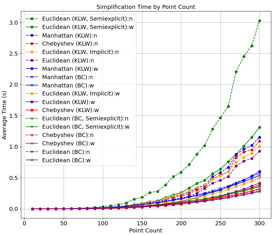
Next, we compare the KLW algorithm (with all optimizations) and the BC algorithm (Figure 7). The KLW algorithm is competitive for polylines of length up to 200, after which the BC algorithm dominates. The BC algorithm’s runtime is smooth due to its rigid structure which yields a cubic running time on all instances.
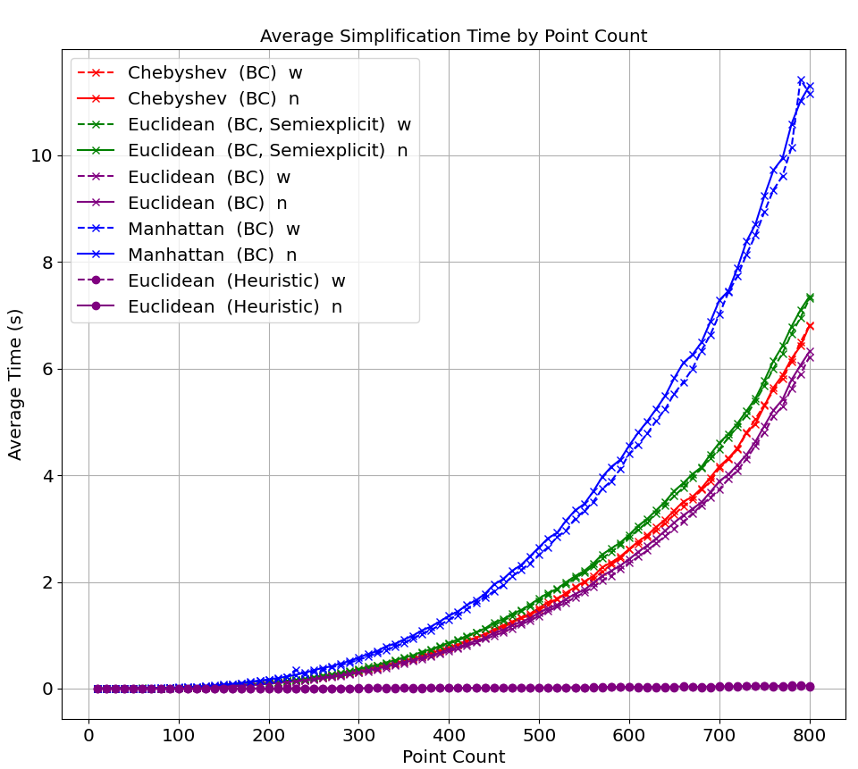
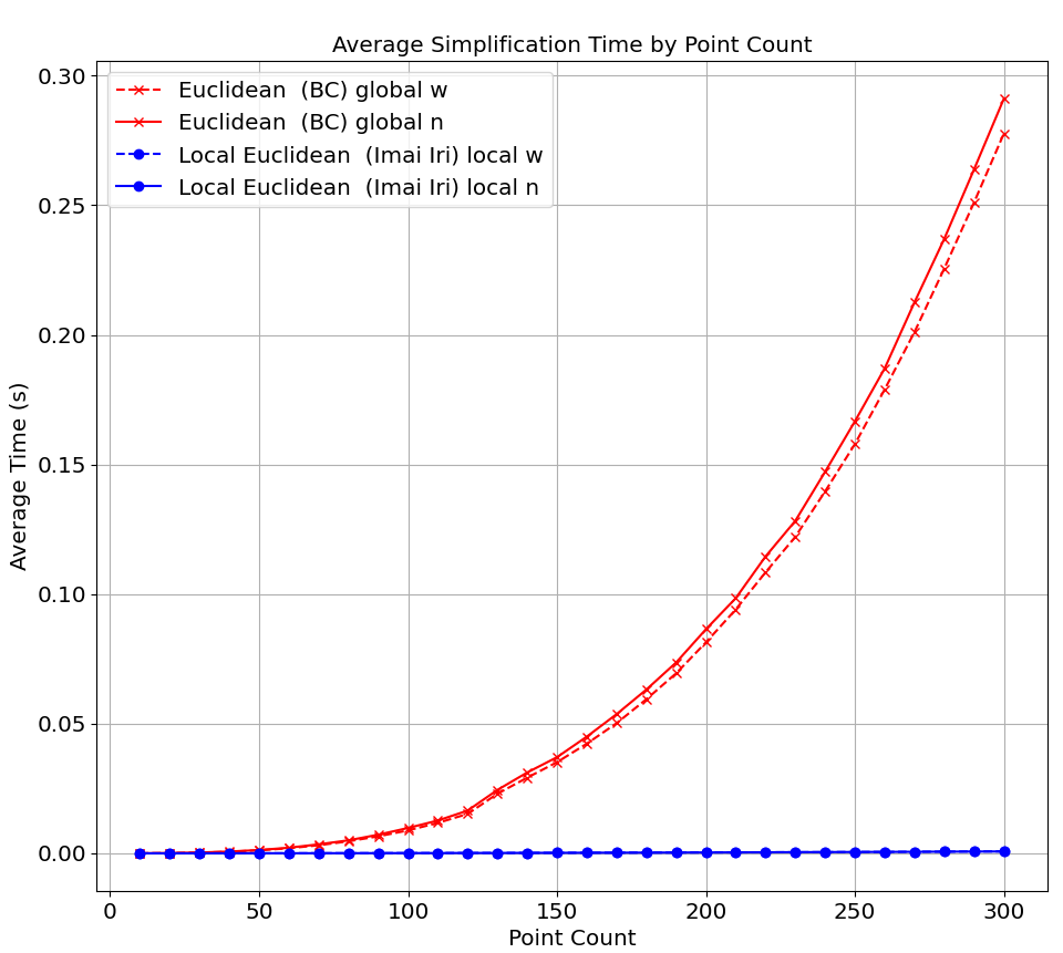
Nevertheless, our implementation allows us to compute exact global simplifications for polylines with up to 800 vertices within a few seconds (see Figure 8). For larger polylines, space consumption becomes the bottleneck on our hardware. On the feasible instances, we also compare the scalability of the BC algorithm and our heuristic in the same figure. The heuristic is approximately 200 times faster, and this speedup grows significantly for larger polylines. Moreover, since the heuristic requires only quadratic space, it can be applied to substantially longer polylines. The heuristic achieved optimal results on all instances, which makes the comparison to the optimal algorithm more fair.
6.3 Simplification Sizes
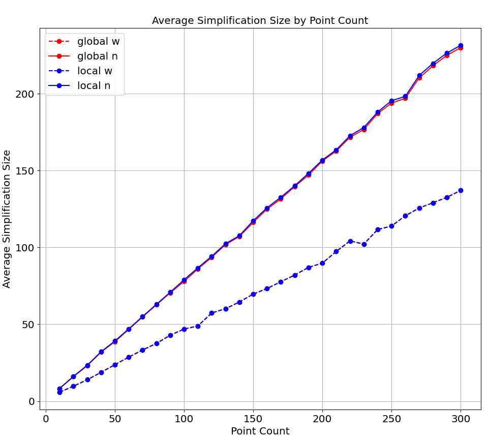
One of the main practical questions is how much global and local simplifications differ on different types of polylines. To answer this, we compare the sizes of optimal global and local simplification of well-behaved and non-well-behaved polylines (Figure 10). The plot contains four data sets, but they are visually difficult to distinguish because the output sizes are, somewhat surprisingly, almost identical for local and global simplification. Indeed, for well-behaved polylines, the sizes were always identical, while for non-well-behaved polylines we observed only marginal differences. The plot also shows that well-behavedness dramatically affects simplification sizes because much longer shortcuts are feasible on well-behaved data. To compute the local simplifications we used a naïve implementation of the Imai-Iri algorithm. This already outperforms the BC algorithm as can be seen in Figure 10.
Given the small difference between global and local simplification sizes, our heuristic (which by construction produces an output size between those two) is nearly always optimal. Testing one million random polylines of length 100, we found only eight instances where the heuristic was non-optimal, with the worst case requiring two extra vertices. By comparison, approximately 10% of these polylines had differing local and global sizes.
To ensure that the similarity between global and local simplification sizes is not an artifact of our parameter choices, we performed an additional experiment with 500000 polylines of 150 vertices each. These were generated with random maximum segment lengths and deviation angles, as well as random . In this experiment, the average difference in size was 0.3 vertices, with a maximum difference of 8 vertices.
6.4 Results on Real Data
Finally, we compare the runtime and the result size of the BC algorithm, the local algorithm and the heuristic on the real-world data using . Here, the heuristic was always optimal. The local simplification was suboptimal on only 5 out of the 400 test cases. We also compute for each the total runtime of the BC algorithm and of the heuristic and show the ratio in Table 2. For small , the heuristic is almost 90 times faster, while for larger it is still 12 times faster than the BC algorithm. We also compare the heuristic against our implementation of the local Imai-Iri algorithm. Surprisingly, it is only 2-4 times slower, which illustrates that the overhead introduced by the interval handling in the heuristic is rather small.
| BC heuristic | heuristic local | |
|---|---|---|
| 2 | 88.24 | 3.86 |
| 8 | 59.26 | 2.96 |
| 32 | 28.04 | 2.65 |
| 128 | 12.40 | 3.13 |
In conclusion, simply using local simplification is the most efficient way to obtain a simplification of good quality in practice (especially as it can be computed even faster than with Imai-Iri [17]). However, our heuristic also scales well and occasionally produces better solutions. On our example instance that illustrates the gap between global and local simplification, the heuristic indeed produces the optimal results.
7 Conclusion and Future Work
Local Fréchet simplifications are known to be globally optimal in 1D. We show that in practice this still holds almost true in 2D on our tested benchmarks. We could only identify meaningful differences to optimal global simplifications in crafted examples. This questions the practical utility of global Fréchet simplification.
Our implicit algorithms are slower than explicit variants but are theoretically more appealing. A practical advantage of them is that, anecdotally, they cause fewer numerical problems that lead to crashes than explicit variants, especially for small and collinear vertices in the polyline. Our semiexplicit variant provides a reasonable trade-off.
There are several open questions that result from this work:
-
Are there practically relevant polyline classes where local and global simplifications differ vastly? Conversely, under which conditions are they similar? For example, on polylines with certain attributes as -packedness [8] or low density [10], it might be possible to prove that local and global simplification sizes are always close.
-
Is our heuristic an approximation? If not, can other splitting/narrowing strategies yield an approximation algorithm outperforming optimal ones?
-
Can local techniques be used to improve the runtime of the exact algorithms or the heuristic? Optimal local simplifications can be computed in near quadratic time [17]. We also derived our algorithms from the Imai-Iri framework. Given this new perspective, local acceleration techniques might become applicable for the global setting.
References
- [1] Pankaj K Agarwal, Sariel Har-Peled, Nabil H Mustafa, and Yusu Wang. Near-linear time approximation algorithms for curve simplification. Algorithmica, 42(3):203–219, 2005. doi:10.1007/S00453-005-1165-Y.
- [2] Helmut Alt and Michael Godau. Computing the Fréchet distance between two polygonal curves. International Journal of Computational Geometry & Applications, 05(01n02):75–91, 1995. doi:10.1142/S0218195995000064.
- [3] Sergey Bereg, Minghui Jiang, Wencheng Wang, Boting Yang, and Binhai Zhu. Simplifying 3d polygonal chains under the discrete Fréchet distance. In Latin American Symposium on Theoretical Informatics, pages 630–641. Springer, 2008. doi:10.1007/978-3-540-78773-0_54.
- [4] Karl Bringmann and Bhaskar Ray Chaudhury. Polyline simplification has cubic complexity. Journal of Computational Geometry, 11(2):94–130, 2021. doi:10.20382/JOCG.V11I2A5.
- [5] Wing Shiu Chan and Francis Chin. Approximation of polygonal curves with minimum number of line segments or minimum error. International Journal of Computational Geometry & Applications, 1996.
- [6] Jacobus Conradi, Ivor van der Hoog, and Eva Rotenberg. On computing the (exact) Fréchet distance with a frog. arXiv preprint arXiv:2512.07728, 2025. doi:10.48550/arXiv.2512.07728.
- [7] David H Douglas and Thomas K Peucker. Algorithms for the reduction of the number of points required to represent a digitized line or its caricature. Cartographica: the international journal for geographic information and geovisualization, 10(2):112–122, 1973.
- [8] Anne Driemel, Sariel Har-Peled, and Carola Wenk. Approximating the Fréchet distance for realistic curves in near linear time. In Proceedings of the twenty-sixth annual symposium on Computational geometry, pages 365–374, 2010. doi:10.1145/1810959.1811019.
- [9] Anne Driemel, Amer Krivošija, and Christian Sohler. Clustering time series under the Fréchet distance. In Proceedings of the twenty-seventh annual ACM-SIAM symposium on Discrete algorithms, pages 766–785. SIAM, 2016. doi:10.1137/1.9781611974331.CH55.
- [10] Joachim Gudmundsson, Zijin Huang, and Sampson Wong. Approximating the -low-density value. In International Computing and Combinatorics Conference, pages 71–82. Springer, 2023. doi:10.1007/978-3-031-49190-0_5.
- [11] Hiroshi Imai and Masao Iri. Computational-geometric methods for polygonal approximations of a curve. Computer Vision, Graphics, and Image Processing, 36(1):31–41, 1986. doi:10.1016/S0734-189X(86)80027-5.
- [12] Georgios Kellaris, Nikos Pelekis, and Yannis Theodoridis. Map-matched trajectory compression. Journal of Systems and Software, 86(6):1566–1579, 2013. doi:10.1016/J.JSS.2013.01.071.
- [13] Hengfeng Li, Lars Kulik, and Kotagiri Ramamohanarao. Spatio-temporal trajectory simplification for inferring travel paths. In Proceedings of the 22nd ACM SIGSPATIAL International Conference on Advances in Geographic Information Systems, pages 63–72, 2014. doi:10.1145/2666310.2666409.
- [14] Kunhui Lin, Zhentuan Xu, Ming Qiu, Xiaoli Wang, and Tianxiong Han. Noise filtering, trajectory compression and trajectory segmentation on GPS data. In 2016 11th International Conference on Computer Science & Education (ICCSE), pages 490–495. IEEE, 2016. doi:10.1109/ICCSE.2016.7581629.
- [15] Xuelian Lin, Shuai Ma, Jiahao Jiang, Yanchen Hou, and Tianyu Wo. Error bounded line simplification algorithms for trajectory compression: An experimental evaluation. ACM Transactions on Database Systems (TODS), 46(3):1–44, 2021. doi:10.1145/3474373.
- [16] Anna Lubiw and András Rácz. A lower bound for the integer element distinctness problem. Information and Computation, 94(1):83–92, 1991. doi:10.1016/0890-5401(91)90034-Y.
- [17] Peter Schäfer, Sabine Storandt, and Johannes Zink. Optimal polyline simplification under the local Fréchet distance in (near-) quadratic time, 2023.
- [18] Mees van de Kerkhof, Irina Kostitsyna, Maarten Löffler, Majid Mirzanezhad, and Carola Wenk. Global curve simplification. In 27th Annual European Symposium on Algorithms (ESA 2019), volume 144, 2019. doi:10.4230/LIPIcs.ESA.2019.67.
- [19] Marc van Kreveld, Maarten Löffler, and Lionov Wiratma. On optimal polyline simplification using the Hausdorff and Fréchet distance. Journal of Computational Geometry, 11(1):1–25, 2020. doi:10.20382/JOCG.V11I1A1.
Appendix A Appendix
A.1 Simplification Data Structure
For a given polyline of length we can construct a data structure that allows to obtain optimal simplification in by precomputing all possible simplifications and performing a binary search111111To actually achieve logarithmic runtime we can only return a reference to a precomputed simplification as a simplification can have linear size.. For this, we note that there is a unique sequence of interval such that , and for any the simplification using needs exactly shortcuts.
We compute the interval boundaries and for each non-empty interval we compute a simplification with which is a valid simplification for all .
To construct the intervals, we construct a set of all possible candidates that can be a boundary for an interval and extract the correct ones in a second step. For the candidates, we consider the implicit relations since they are sufficient to implement a simplification algorithm. A simplification size can only change if the result of at least one decision changes. The wait and proceed relation depend on one line segment and two vertices. There are possibilities to choose such an edge and two vertices (in total four vertices); thus we only need to determine how many candidates there are for each combination of four vertices.
Fix a line segment and two vertices . The candidates for are values at which the result of the wait or proceed relation changes. This happens when the relative position of the solutions and changes. This happens for such that . Intuitively, consider the Voronoi diagram for the vertices and . The result of the relations only changes on the boundary between the two cells. Thus, we need the intersections of this boundary with the line segment. In the Euclidean case, this intersection is a unique point, empty or an interval (if the line segment lies exactly on the boundary). Only in the case where it is a unique point does the result of the decision change and thus there are many candidates in the Euclidean case.
For the Manhattan and Chebyshev case, there may be many intersections and thus candidates. Other Minkowski distances are even more complicated. We only consider and the Euclidean, Manhattan, and Chebyshev case which have candidates.
After we have found all candidates, we can sort them and perform for each simplification length a binary search to find the respective interval boundary. This takes in total to sort. To compare the simplification sizes per pair of candidates, we compute the simplifications in . As each binary search needs simplification calls, the total runtime is still .
The space consumption is due to the candidates. This can be reduced to a cubic space consumption using the following trick: Use a sweep line algorithm and compute the candidates in order. For each line segment, the candidate events correspond to a line intersection-like problem121212We actually compute intersections of more complicated curves and not just line segments but the main idea is the same. which can be solved similarly to the Bentley-Ottmann algorithm. With this, we can compute the events in order. Compute candidates, perform binary search, discard the current batch of candidates and proceed to ensure cubic space consumption.
Interestingly, the equation for the euclidean distance simplifies to a linear equation. Thus, no candidate requires square root computations and thus, using an implicit simplification algorithm, the construction of this data structure can be done without square roots. Moreover, the same approach applies to the local setting. Here, only quadratically many candidates are necessary ( for each shortcut ).
A.2 Equation Solving Lower Bounds
For the algorithm in Section A.1, we need to solve equations of the form for line segment , and points . With the Euclidean distance, they are trivial to solve and have at most one solution (or one closed interval). Using the Manhattan or Chebyshev distance, these equations are more complicated but it is possible to find algorithms for both. As an interesting theoretical question, we were able to establish matching lower bounds for both of them using a reduction to integer element distinctness as introduced by Lubiw and Rácz [16].
Definition 10 (Integer Element Distinctness).
Given integers . Decide if there exist indices such that .
This problem has a known lower bound of due to Lubiw and Rácz.
For the Chebyshev case, we are given . Let be a large constant that we specify later. Define the linear function , which is the tangent of at . Note that for all . We construct the equation .
This means the functions and consist of exactly distinct line segments, where is the number of distinct elements in , as each distinct value contributes one segment. From to , the segments are encountered in descending order of . The last segment is encountered at least after , since the smallest is 2, so .
If all linear functions are positive on , then the absolute values can be removed, and and equal the left and right sides of this equation, respectively. For , it can be verified that all terms are positive on .
Now, consider the equation on . At , we have , and at , we have for all . Let be the number of distinct . There are at least solutions because the sign of alternates between these points. However, there cannot be more than solutions because each of the segments in can intersect the piecewise linear function at most twice (since both are convex, and the first and last segments cannot both intersect twice). Thus, the number of solutions in is exactly . For an example refer to Figure 12.
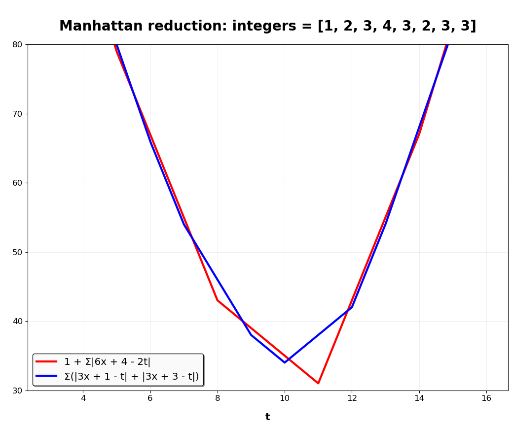
For the Manhattan case, given an instance of the integer element distinctness problem , we construct an instance of the Manhattan equation problem in dimensions as
Observe that for , we have . For , we have . Furthermore, for any , the equation has exactly two solutions in .
Let and . For for any , we have . For , the difference , where is the multiplicity of , has exactly two solutions in the interval. Thus, the total number of solutions is , where is the number of distinct values in . Therefore, solving the Manhattan equation problem allows us to determine , and hence the lower bound applies. For an example refer to Figure 12.