ZOR Filters: Fast and Smaller Than Fuse Filters

We briefly recap Fuse filter construction to fix notation and to separate prior work [19] from our contributions.

We consider a static set $S$ of $n$ distinct keys and an array of $m$ cells. Each key $x\in S$ is mapped, via hashing, to $N$ cells

The filter stores in each cell an $F$-bit value (a “cell fingerprint”) and answers a membership query for $y$ by combining the $N$ cell values at $H(y)$ by bitwise XOR and comparing against a fingerprint of $y$ [18, 19]. Fuse filters differ from XOR filters primarily in how $H(x)$ is chosen to improve locality and construction speed. The array is partitioned into many disjoint segments, and $H(x)$ consists of one location in each of $N$ consecutive segments. In practice segments are sized as powers of two to accelerate range reduction. This “consecutive-segment” constraint improves cache behaviour during both query and construction and also reduces the required overhead ($m/n$) for successful peeling.

Construction proceeds in two stages. First, each cell records which keys map to it: for every $x\in S$, we insert $x$ into the incidence lists of all cells in $H(x)$. Equivalently, this defines a hypergraph whose vertices are the $m$ cells and whose hyperedges are the keys, each hyperedge connecting the $N$ vertices $H(x)$. Second, the algorithm performs a peeling process. We iteratively search for any cell $v$ that currently contains a unique key (i.e., whose current degree is $1$). If such a cell exists, let $x$ be its unique incident key. We link $x$ to $v$ (recording that $x$ will later be resolved at $v$), and remove all occurrences of $x$ from the other cells in $H(x)\setminus \{v\}$, updating their degrees. This removal can create new cells of degree $1$, which are then processed in the same way. The procedure continues until either every key has been linked, or no cell of degree $1$ exists while unprocessed keys remain; in that case the construction fails and is typically restarted with different hash seeds.

Once a full linking order exists (i.e., all keys have been peeled), the cell payloads are assigned in reverse order. Let $f(\cdot )$ be an $F$-bit fingerprint function. When processing a key $x$ linked to cell $v\in H(x)$, all other incident cell values have already been fixed; we set

so that ${⨁}_{u\in H(x)}T[u]=f(x)$. This completes the construction.

The core issue of XOR/Fuse peeling is that the process can get stuck on a remaining subgraph in which every still-active cell has degree at least $2$ (i.e., no degree-$1$ cell exists), which forces a complete restart in the standard algorithm. Our solution avoids restarts by using an always-terminating variant that abandons keys whenever the process blocks. Allowing a controlled false-negative rate has precedent in other filtering settings, e.g., stable Bloom filters for streaming where older items are intentionally forgotten [8] and retouched Bloom filters that trade false negatives for fewer false positives [14]. Our main goal here is different: we use such filters as an intermediate object and then recover standard false-positive-only semantics via an auxiliary structure.

Formally, we follow the Fuse construction algorithm, but we modify the step taken when the queue of degree-$1$ cells becomes empty while keys remain. Instead of restarting, we select a cell $v$ with minimal current degree

and consider the $d_{\min }$ keys currently incident to $v$. We keep one key $x^{\star }$ (to be resolved at $v$) and abandon the other $d_{\min }-1$ keys by removing them from all their incident cells. After this forced removal, cell $v$ becomes degree $1$ and the usual peeling step can proceed without restarting. This forced removal decreases degrees and guarantees progress. Repeating this rule ensures termination because each step removes at least one still-active key from the incidence structure.

Let $A\subseteq S$ denote the abandoned set and $\alpha =|A|/n$ the abandoned fraction. The main structure is then constructed exactly as a Fuse filter, but only for $S\setminus A$. This main structure alone is an approximate filter with both false positives (as in a Fuse filter) and false negatives (on keys in $A$). We refer to this single-stage object (without an auxiliary) as a pure ZOR filter. Pure ZOR filters are interesting in their own right when a very small false-negative rate is acceptable (in our measurements often below the $1\%$ scale), but the main goal of this work is to recover the standard false-positive-only semantics. We propose to achieve this by explicitly handling $A$ with an auxiliary structure.

A practical consequence of always-terminating construction is that it removes restart-driven uncertainty: for a fixed array size $m$, construction never fails, and the “difficulty” of the instance manifests as $\alpha$ rather than as a rebuild probability. In particular, if one chooses $m=n$ (one cell per key), then the main structure uses exactly $F$ bits per original key; choosing $m>n$ reduces the abandoned fraction at the cost of a multiplicative space factor $m/n$, whereas choosing yields a cheaper main structure but necessarily increases false negatives. In the following, we choose $m=n$ because it minimises the main-structure footprint for our intended use; we leave the study of other $m/n$ trade-offs to future work.

When the peel queue is empty, the algorithm must force progress on a remaining core in which all active cells have degree at least $2$. It does so by selecting an intervention cell $v$ and processing all currently active keys incident to $v$: exactly one key is kept and will be resolved at $v$, while the remaining $d(v)-1$ incident keys are abandoned and removed from the incidence structure. A consequence is that, once $v$ is chosen, all keys incident to $v$ disappear from the active structure (either as kept or abandoned). Therefore, the subsequent evolution of degrees is governed mainly by the choice of the intervention cell $v$; the choice of which single key to keep affects only which key remains in $S\setminus A$ (and hence which key does not require auxiliary handling).

Accordingly, we choose $v$ among currently minimal-degree cells so as to minimise the number of abandoned keys created by each intervention. This is a local choice based only on the current degrees and incidences, and it does not guarantee a globally minimal abandoned set. Let $ℐ(v)$ be the set of currently active keys incident to $v$, and let $d(u)$ be the current degree of a cell $u$. Intervening at $v$ removes every key in $ℐ(v)$ from each of its other incident cells, i.e., from cells in

A simple proxy for how much this intervention will “unlock” the peel process is how many degree-$2$ neighbours are hit, since decreasing a degree-$2$ cell by one creates a new degree-$1$ cell. We capture this with

When multiple candidates have similar $\mathrm{deg2}(v)$, we use secondary scores to prefer interventions whose impact is concentrated in lighter neighbourhoods. With multiplicity over incidences, define

and let $\mathrm{vec}(v)$ be the multiset of degrees $\{d(u):u\in H(x)\setminus \{v\},x\in ℐ(v)\}$ sorted in non-decreasing order.

In our implementation, when a blocking event occurs we scan up to $T$ distinct minimal-degree cells. For each scanned candidate $v$ we compute the scores above, then pick the best-scoring candidate under a chosen policy. This parameter $T$ controls the extra work spent per blocking event. We implemented the following intervention policies (all restricted to cells of minimal current degree, or to the best among the $T$ scanned minimal-degree candidates):

• $\mathrm{■}$

  Lightest-neighbourhood: minimise $\mathrm{sum}(v)$; break ties by larger $\mathrm{deg2}(v)$, then smaller $\max (v)$.

• $\mathrm{■}$

  Heaviest-neighbourhood: maximise $\mathrm{sum}(v)$; break ties by smaller $\mathrm{deg2}(v)$, then larger $\max (v)$.

• $\mathrm{■}$

  MostDeg2: compare $\mathrm{vec}(v)$ lexicographically (preferring smaller degrees earlier); break ties by larger $\mathrm{deg2}(v)$, then smaller $\mathrm{sum}(v)$ and smaller $\max (v)$.

• $\mathrm{■}$

  MinMaxDegree: minimise $\max (v)$; break ties by smaller $\mathrm{sum}(v)$, then larger $\mathrm{deg2}(v)$.

Once $v$ is selected, the choice of the single kept key among $ℐ(v)$ is made deterministically (e.g., by a fixed hash order) for reproducibility.

Pure ZOR filters may return false negatives precisely on the abandoned set $A$. To recover the standard false-positive-only semantics, we store the abandoned keys that would otherwise be missed by the main structure in an auxiliary static structure, such as a Fuse filter or an MPHF-plus-fingerprint table. Concretely, we define $A^{\prime }\subseteq A$ as the subset of abandoned keys for which the main structure returns “absent” at build time (see Section 2.6 for more details); storing $A^{\prime }$ suffices to eliminate false negatives.

Let the main filter have false-positive probability ${\epsilon }_1$ and the auxiliary have false-positive probability ${\epsilon }_2$. We answer membership queries by checking the main structure first and consulting the auxiliary only if needed. A query returns “present” if either structure matches, hence the overall false-positive probability is

and the difference is ${\epsilon }_1{\epsilon }_2$, which is negligible when ${\epsilon }_1,{\epsilon }_2\ll 1$. The next subsections detail auxiliary sizing and practical handling choices before discussing query-path layout.

A natural question is how large the auxiliary fingerprint should be to minimise space at a target overall error. For this analysis, we ignore implementation-specific constants and measure only fingerprint bits. The main filter stores $F$ bits per original key when $m=n$, the auxiliary stores $G$ bits per auxiliary-stored key, and the abandoned fraction is $\alpha$, so the total bits per original key are

Under the standard fingerprint model, ${\epsilon }_1\simeq 2^{-F}$ and ${\epsilon }_2\simeq 2^{-G}$, and therefore

Define the multiplicative overhead relative to the information-theoretic bound as

Optimising under the approximation ${\epsilon }_{\mathrm{tot}}\approx 2^{-F}+2^{-G}$ yields the balance condition

with a detailed derivation provided in Appendix A.

Thus, the auxiliary false-positive rate should be on the order of $\alpha$ times the main false-positive rate. In practice we take the ceiling, for example

For $\alpha =1\%$, ${\log }_2(1/\alpha )={\log }_2(100)\approx 6.64$, suggesting $G^{\star }\approx F+7$. In our experiments, $\alpha$ is often below $1\%$ for moderate arity (e.g., $N\ge 5$), so we use $G=F+8$ as a simple default that keeps ${\epsilon }_2$ negligible, remaining close to optimal while being efficient in practice.

Before inserting an abandoned key $x\in A$ into the auxiliary filter, we may query the main filter on $x$. If the main filter already returns “present” for $x$, then $x$ will not be a false negative at query time and does not require auxiliary handling. Under a uniform fingerprint model, this happens with probability approximately ${\epsilon }_1$. This optimisation is negligible for low ${\epsilon }_1$ (large fingerprints) but can be noticeable for small $F$ (especially below 8 bits). Overall, this optimisation can reduce the auxiliary size, especially when $F$ is small, at the modest build-time cost of one extra main-filter query per abandoned key.

Instead of using a single auxiliary filter, a natural idea would be to cascade stages: build a primary ZOR structure on $S$, then build a second-stage structure on the abandoned keys, and repeat until the remainder is small enough to be handled by a different representation (e.g., a tiny exact set or a final conventional filter). If the first stage abandons a fraction ${\alpha }_1$ of the original keys and the second stage abandons a fraction ${\alpha }_2$ of its input, then the size of the remaining set after two stages is ${\alpha }_1{\alpha }_{2}n$. Consequently, the space contribution of later stages shrinks multiplicatively: a third stage contributes a term proportional to ${\alpha }_1{\alpha }_2$, and so on.

Cascading can therefore reduce the auxiliary footprint, but the gain is typically limited when ${\alpha }_1$ is already small, while query time increases because negative queries may need to check multiple stages. This trade-off is particularly clear in our current design, where the auxiliary is implemented as a 4-wise Fuse filter with multiplicative overhead $1.075$ over the information-theoretic bound [19]. With a main ZOR fingerprint of $F$ bits and auxiliary fingerprints of $F+8$ bits, the auxiliary contributes an overhead (relative to $F$) of approximately

For instance, with ${\alpha }_1=0.5\%$ and $F=16$, this evaluates to

If one adds a second ZOR stage before the final Fuse auxiliary (i.e., ZOR+ZOR+FUSE), and if the second stage can itself be implemented at about $1\%$ overhead over its own information-theoretic target, then the effective overhead factor for handling the abandoned keys becomes roughly $1.01$ instead of $1.075$ for that portion. This yields the approximation

which for the same ${\alpha }_1=0.5\%$ and $F=16$ gives

Thus, cascading replaces an overhead around $0.81\%$ by about $0.76\%$ in this representative regime: the absolute gain is small because the auxiliary is already weighted by ${\alpha }_1$. This is the main practical limitation of cascading in our setting: once ${\alpha }_1$ is below the percent level, additional stages offer diminishing space returns but impose a direct cost in query time, since negatives may need to evaluate more stages before rejecting. Accordingly, we use a single auxiliary stage in the experiments and treat cascading mainly as an optional refinement for cases where query-time budgets are less stringent or when most queries are positive. Moreover, even if the abandoned keys were handled at the information-theoretic limit (i.e., with exactly $G$ bits per abandoned key to match a $2^{-G}$ target), the auxiliary would still cost at least $\alpha G$ additional bits per original key, so the multiplicative space overhead has a hard lower bound of $\alpha$. In other words, once $\alpha$ is already small, the dominant lever for further space improvements is not adding stages but reducing $\alpha$ itself (e.g., by increasing arity, tuning segment parameters, or improving the abandonment policy), because every auxiliary term is multiplied by $\alpha$ and therefore exhibits diminishing returns from additional cascading.

If the auxiliary were stored as a fully separate structure, negative queries would typically perform one random access in the main filter and then a second unrelated random access in the auxiliary. Since negatives trigger the auxiliary with probability close to $1-{\epsilon }_1$, this organization would make two random cache misses common on negative lookups.

To mitigate this effect, we use an interleaved layout for the main and auxiliary structures. Construction proceeds in three stages: (i) build the main ZOR structure on $S\setminus A$, (ii) build the auxiliary Fuse structure on $A^{\prime }$, and (iii) interleave both probe layouts using a shared hash seed and aligned index families. This design makes both stages use related probe indices and nearby memory locations.

At query time, the shared probe indices are computed once. The main stage is evaluated first; only if it returns “absent” is the auxiliary stage evaluated at the corresponding interleaved locations. Because auxiliary cells are colocated with main cells for the same indices, the second-stage accesses are often served from nearby cache lines. Thus, the interleaved layout is designed to minimize additional cache misses, replacing a second unrelated random access in many negative queries with mostly in-cache work.

A key to the extremely fast Fuse-filter construction is that the builder can avoid explicit adjacency lists during peeling because the algorithm only ever removes degree-$1$ cells. Each cell can maintain just two aggregates: a degree counter and the XOR of the hashes of incident keys. When a cell reaches degree $1$, the XOR aggregate reveals the unique remaining key, enabling the builder to continue without knowing the full incidence list. If peeling gets stuck in a core, Fuse construction simply restarts with a new seed, so it never needs to identify and delete a specific key from a multi-degree cell.

During ZOR construction when the peel queue is empty, it must choose a key to abandon from a cell with degree at least $2$. At that moment, the count+XOR trick is insufficient because it does not identify which active key should be removed, nor does it support enumerating the incident keys. The builder therefore needs per-cell membership information (an adjacency list or an equivalent structure) to locate an active key and update all its incident cells. This additional structure increases memory traffic and random access during peeling, which explains why the current ZOR implementation is slower to build even though query evaluation remains similar to Fuse filters.

Unless stated otherwise, experiments use the same generated key universe and fixed seeds across methods; keys are generated once and reused. Construction-scaling benchmarks use prefixes of the same key set from $2^{18}$ to $2^{28}$ keys.

We start by measuring the abandoned fraction $\alpha$ as a function of the arity $N$ (number of hash functions) and the set size $n$ (Figure 1, left). Increasing $N$ reduces $\alpha$ up to diminishing returns above $5$, and larger sets tend to improve behaviour, consistent with prior observations for XOR- and Fuse-style peeling constructions. For the largest sets we tested, the measured abandonment rates were $6.1\%$ (3-wise), $2.1\%$ (4-wise), $0.9\%$ (5-wise), $0.6\%$ (6-wise), $0.5\%$ (7-wise), and $0.4\%$ (8-wise). Thus, abandonment below $1\%$ is achievable in practice with $N\ge 5$, so the auxiliary handles at most $\alpha n$ keys, about two orders of magnitude fewer keys than the main structure. In the pure ZOR setting (without an auxiliary), these values also correspond directly to very low false-negative rates.

We also study the segment (block) size used for Fuse-style hashing (Figure 1, right). As in Fuse filters, we observe an intermediate segment size that minimises abandonment, reflecting a trade-off between locality (small segments) and effective randomness in the induced hypergraph (large segments).

We then compare memory cost and relative overhead in a frontier-style view (Figure 2): both panels use $x=-{\log }_2(\epsilon )$. Figure 2 (left) reports bits per key, and Figure 2 (right) reports overhead relative to the information-theoretic target $x$. The plot includes ZOR points (Z2/Z4/Z8), Fuse references (F3/F4), an MPHF reference curve, and only the BuRR-0.1% baseline from our benchmark runs (explicitly at each fingerprint size $b\in \{4,8,16,24,32\}$) [19, 12]. BuRR-0.1% is an aggressive BuRR overhead setting and is included as a representative low-overhead BuRR baseline.

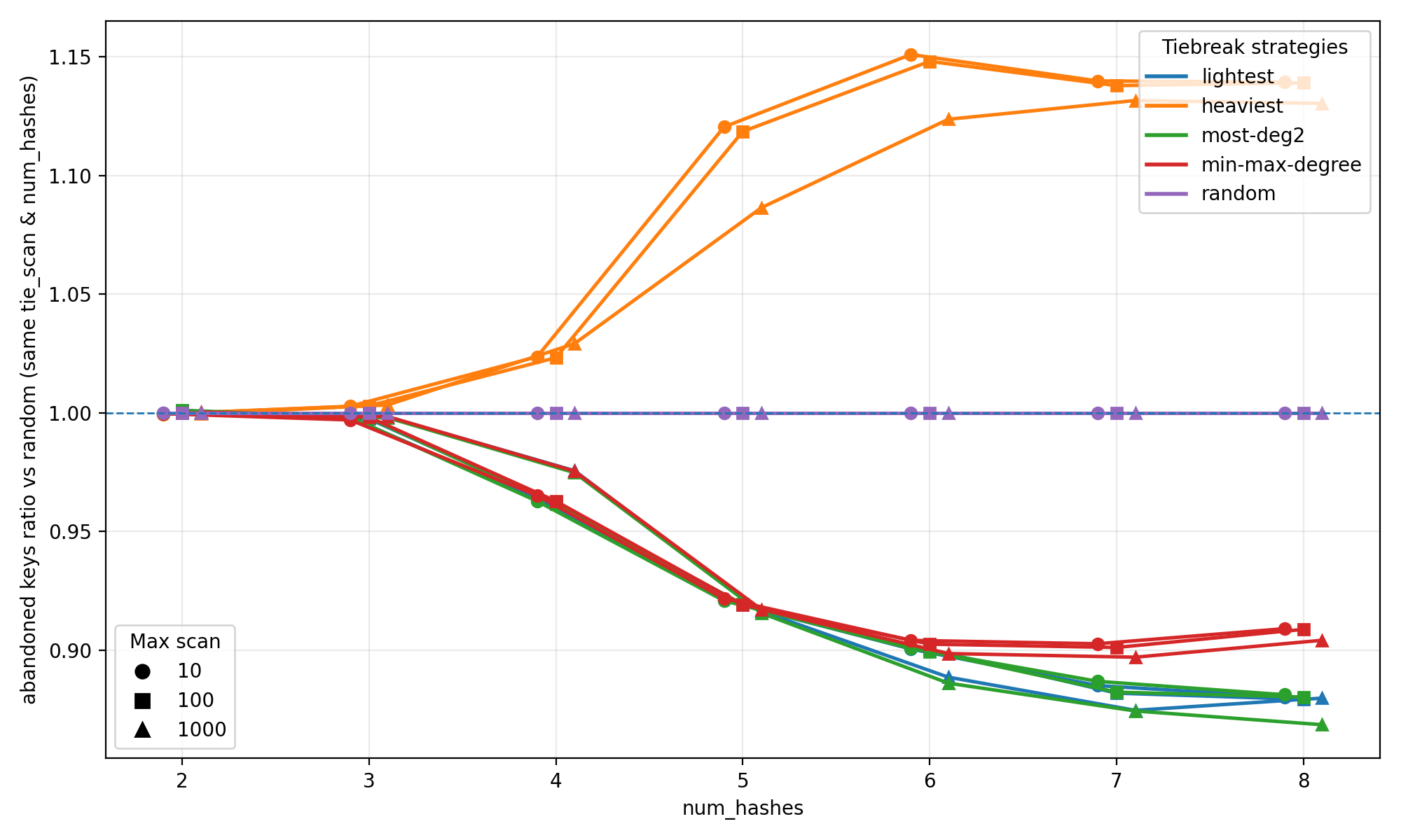
Next, we evaluate tie-breaking strategies for choosing an intervention cell at blocking events (Figure 3). Compared to a random choice, the degree-based heuristics reduce the abandoned fraction in our experiments, while some strategies can also increase $\alpha$ depending on arity and scan budget. Increasing T yields modest additional gains but can noticeably increase build time, especially at low arity.

We then evaluate query performance in nanoseconds per query at two false-positive targets, $\epsilon \approx 2^{-8}$ and $\epsilon \approx 2^{-16}$ (Figure 4). For each target, the left panel reports single-threaded query execution (1 core), and the right panel reports multithreaded execution (32 cores). Across both targets, ZOR-pure remains closest to Fuse-4 on positive-query latency. The complete ZOR variant shown as ZOR trades additional negative-query latency for deterministic continuation and low overhead. Compared with BuRR-10%, BuRR-1%, and BuRR-0.1%, both ZOR variants (ZOR and ZOR-pure) are clearly faster on positive queries in both single-threaded and multithreaded settings at both targets. For negative queries, ZOR-pure is also faster than the BuRR baselines across both targets. By contrast, ZOR is slower than BuRR at $\epsilon \approx 2^{-8}$, while at $\epsilon \approx 2^{-16}$ it is faster than BuRR in the single-threaded panel but slower in the 32-threaded panel. All complete-ZOR bars use the interleaved main/aux query path defined in Section 2.8. Because positive queries are usually resolved in the main stage, their latency stays closer to Fuse-4 and ZOR-pure, while negatives more often trigger the auxiliary path.

Finally, we evaluate construction scaling over growing set sizes from $2^{18}$ to $2^{28}$ keys (Figure 6) using the construction baseline set above. To focus the comparison, we report wall-clock construction time only (log-log scale). The results confirm that ZOR-4 and ZOR-8 construction remain slower than Fuse-4 and the BuRR baselines at equal false-positive target [19, 12], while preserving deterministic termination and low space overhead. This gap is now concentrated in the construction kernel and motivates further implementation work on memory traffic and parallel peeling efficiency.

To characterise partitioned-build parallelism directly, we also benchmark partitioned ZOR construction across every partition/core setting from $1$ to $32$ (Figure 5). Using fixed $200$M keys and arity $N=8$, build time decreases from $244.404$s at $1$ partition to $24.038$s at $32$ partitions, i.e., about $10.17\times$ speedup. The measured curve is close to linear at low partition counts and then progressively flattens as partition count grows, consistent with memory-bandwidth and synchronisation limits near full-core utilisation.

The main limitation of the current implementation is construction speed. In our benchmarks, ZOR construction is still slower than highly optimised Fuse/BuRR builders [19, 12], mainly because deterministic progress in blocked peeling phases requires explicit incidence maintenance and updates. Future work is therefore primarily engineering-focused: reducing memory traffic during peeling, improving adjacency representations, and adopting segment-local buffering and vectorised hashing in the style of optimised Fuse/BuRR builders. Algorithmic directions include improved abandonment policies, exploration of sizing choices ($m/n$) as a space/time/abandonment trade-off, query-side optimisations that reduce auxiliary checks for negative queries, and a more systematic study of pure ZOR filters for applications where a tiny false-negative rate is acceptable.

References

- [1] Michael A Bender, Martin Farach-Colton, Rob Johnson, Bradley C Kuszmaul, Dzejla Medjedovic, Pablo Montes, Pradeep Shetty, Richard P Spillane, and Erez Zadok. Don’t thrash: How to cache your hash on flash. In 3rd Workshop on Hot Topics in Storage and File Systems (HotStorage 11), 2011. doi:10.48550/arXiv.1208.0290.
- [2] Burton H Bloom. Space/time trade-offs in hash coding with allowable errors. Communications of the ACM, 13(7):422–426, 1970. doi:10.1145/362686.362692.
- [3] Alex D Breslow and Nuwan S Jayasena. Morton filters: faster, space-efficient cuckoo filters via biasing, compression, and decoupled logical sparsity. Proceedings of the VLDB Endowment, 11(9):1041–1055, 2018. doi:10.14778/3213880.3213884.
- [4] Andrei Broder and Michael Mitzenmacher. Network applications of bloom filters: A survey. Internet mathematics, 1(4):485–509, 2004. doi:10.1080/15427951.2004.10129096.
- [5] Fay Chang, Jeffrey Dean, Sanjay Ghemawat, Wilson C Hsieh, Deborah A Wallach, Mike Burrows, Tushar Chandra, Andrew Fikes, and Robert E Gruber. Bigtable: A distributed storage system for structured data. ACM Transactions on Computer Systems (TOCS), 26(2):1–26, 2008. doi:10.1145/1365815.1365816.
- [6] Rayan Chikhi, Téo Lemane, Raphaël Loll-Krippleber, Mercè Montoliu-Nerin, Brice Raffestin, Antonio Pedro Camargo, Carson J Miller, Mateus Bernabe Fiamenghi, Daniel Paiva Agustinho, Sina Majidian, et al. Logan: planetary-scale genome assembly surveys life’s diversity. bioRxiv, pages 2024–07, 2025. doi:10.1101/2024.07.30.605881.
- [7] Niv Dayan, Manos Athanassoulis, and Stratos Idreos. Optimal bloom filters and adaptive merging for lsm-trees. ACM Transactions on Database Systems, 43(4):1–48, 2018. doi:10.1145/3276980.
- [8] Fan Deng and Davood Rafiei. Approximately detecting duplicates for streaming data using stable bloom filters. In Proceedings of the 2006 ACM SIGMOD international conference on Management of data, pages 25–36, 2006. doi:10.1145/1142473.1142477.
- [9] Sarang Dharmapurikar, Praveen Krishnamurthy, and David E Taylor. Longest prefix matching using bloom filters. In Proceedings of the 2003 conference on Applications, technologies, architectures, and protocols for computer communications, pages 201–212, 2003. doi:10.1145/863955.863979.
- [10] Sarang Dharmapurikar, Haoyu Song, Jonathan Turner, and John Lockwood. Fast packet classification using bloom filters. In Proceedings of the 2006 ACM/IEEE symposium on Architecture for networking and communications systems, pages 61–70, 2006. doi:10.1145/1185347.1185356.
- [11] Martin Dietzfelbinger and Rasmus Pagh. Succinct data structures for retrieval and approximate membership. In International Colloquium on Automata, Languages, and Programming, pages 385–396. Springer, 2008. doi:10.1007/978-3-540-70575-8_32.
- [12] Peter C. Dillinger, Lorenz Hübschle-Schneider, Peter Sanders, and Stefan Walzer. Fast succinct retrieval and approximate membership using ribbon. In 20th International Symposium on Experimental Algorithms (SEA 2022), volume 233 of LIPIcs, pages 4:1–4:20. Schloss Dagstuhl – Leibniz-Zentrum für Informatik, 2022. Software repository: https://github.com/lorenzhs/BuRR. doi:10.4230/LIPIcs.SEA.2022.4.
- [13] Peter C Dillinger and Stefan Walzer. Ribbon filter: practically smaller than bloom and xor. arXiv preprint arXiv:2103.02515, 2021. doi:10.48550/arXiv.2103.02515.
- [14] Benoit Donnet, Bruno Baynat, and Timur Friedman. Retouched bloom filters: allowing networked applications to trade off selected false positives against false negatives. In Proceedings of the 2006 ACM CoNEXT conference, pages 1–12, 2006. doi:10.1145/1368436.1368454.
- [15] David Eppstein. Cuckoo filter: Simplification and analysis. arXiv preprint arXiv:1604.06067, 2016. doi:10.48550/arXiv.1604.06067.
- [16] Bin Fan, Dave G Andersen, Michael Kaminsky, and Michael D Mitzenmacher. Cuckoo filter: Practically better than bloom. In Proceedings of the 10th ACM International on Conference on emerging Networking Experiments and Technologies, pages 75–88, 2014. doi:10.1145/2674005.2674994.
- [17] Li Fan, Pei Cao, Jussara Almeida, and Andrei Z Broder. Summary cache: a scalable wide-area web cache sharing protocol. IEEE/ACM transactions on networking, 8(3):281–293, 2000. doi:10.1109/90.851975.
- [18] Thomas Mueller Graf and Daniel Lemire. Xor filters: Faster and smaller than bloom and cuckoo filters. Journal of Experimental Algorithmics (JEA), 25:1–16, 2020. doi:10.1145/3376122.
- [19] Thomas Mueller Graf and Daniel Lemire. Binary fuse filters: Fast and smaller than xor filters. Journal of Experimental Algorithmics (JEA), 27(1):1–15, 2022. doi:10.1145/3510449.
- [20] Sven Groppe, Thomas Kiencke, Stefan Werner, Dennis Heinrich, Marc Stelzner, and Le Gruenwald. P-luposdate: using precomputed bloom filters to speed up sparql processing in the cloud. Open Journal of Semantic Web (OJSW), 1(2):25–55, 2014. No DOI registered (checked on April 10, 2026). URL: https://nbn-resolving.org/urn:nbn:de:101:1-201705194858.
- [21] Robert S Harris and Paul Medvedev. Improved representation of sequence bloom trees. Bioinformatics, 36(3):721–727, 2020. doi:10.1093/bioinformatics/btz662.
- [22] Stefan Hermann, Hans-Peter Lehmann, Giulio Ermanno Pibiri, Peter Sanders, and Stefan Walzer. Phobic: Perfect hashing with optimized bucket sizes and interleaved coding. In 32nd Annual European Symposium on Algorithms (ESA 2024), Leibniz International Proceedings in Informatics (LIPIcs), 2024. doi:10.4230/LIPIcs.ESA.2024.69.
- [23] Yohan Hernandez-Courbevoie, Mikaël Salson, Chloé Bessière, Haoliang Xue, Daniel Gautheret, Camille Marchet, and Antoine Limasset. Reindeer2: Practical abundance index at scale. In International Symposium on String Processing and Information Retrieval (SPIRE 2025), Lecture Notes in Computer Science, pages 156–171. Springer, 2025. doi:10.1007/978-3-032-05228-5_14.
- [24] Avinash Lakshman and Prashant Malik. Cassandra: a decentralized structured storage system. ACM SIGOPS operating systems review, 44(2):35–40, 2010. doi:10.1145/1773912.1773922.
- [25] Harald Lang, Thomas Neumann, Alfons Kemper, and Peter Boncz. Performance-optimal filtering: Bloom overtakes cuckoo at high throughput. Proceedings of the VLDB Endowment, 12(5):502–515, 2019. doi:10.14778/3303753.3303757.
- [26] Taewhi Lee, Kisung Kim, and Hyoung-Joo Kim. Join processing using bloom filter in mapreduce. In Proceedings of the 2012 ACM Research in Applied Computation Symposium, pages 100–105, 2012. doi:10.1145/2401603.2401626.
- [27] Hans-Peter Lehmann, Thomas Mueller, Rasmus Pagh, Giulio Ermanno Pibiri, Peter Sanders, Sebastiano Vigna, and Stefan Walzer. Modern minimal perfect hashing: A survey. ACM Computing Surveys, 58(10):1–36, 2026. doi:10.1145/3797036.
- [28] Antoine Limasset, Guillaume Rizk, Rayan Chikhi, and Pierre Peterlongo. Fast and scalable minimal perfect hashing for massive key sets. In 24th International Symposium on Experimental Algorithms (SEA 2017), volume 75 of LIPIcs, pages 25:1–25:16. Schloss Dagstuhl – Leibniz-Zentrum für Informatik, 2017. doi:10.4230/LIPIcs.SEA.2017.25.
- [29] Lothar F Mackert and Guy M Lohman. R* optimizer validation and performance evaluation for local queries. ACM SIGMOD Record, 15(2):84–95, 1986. doi:10.1145/16856.16863.
- [30] Camille Marchet, Mael Kerbiriou, and Antoine Limasset. Blight: efficient exact associative structure for k-mers. Bioinformatics, 37(18):2858–2865, 2021. doi:10.1093/bioinformatics/btab217.
- [31] Camille Marchet, Lolita Lecompte, Antoine Limasset, Lucie Bittner, and Pierre Peterlongo. A resource-frugal probabilistic dictionary and applications in bioinformatics. Discrete Applied Mathematics, 274:92–102, 2020. doi:10.1016/j.dam.2018.03.035.
- [32] Camille Marchet and Antoine Limasset. Scalable sequence database search using partitioned aggregated bloom comb trees. Bioinformatics, 39(Supplement_1):i252–i259, 2023. doi:10.1093/bioinformatics/btad225.
- [33] Patrick O’Neil, Edward Cheng, Dieter Gawlick, and Elizabeth O’Neil. The log-structured merge-tree (lsm-tree). Acta informatica, 33(4):351–385, 1996. doi:10.1007/s002360050048.
- [34] Prashant Pandey, Alex Conway, Joe Durie, Michael A Bender, Martin Farach-Colton, and Rob Johnson. Vector quotient filters: Overcoming the time/space trade-off in filter design. In Proceedings of the 2021 International Conference on Management of Data, pages 1386–1399, 2021. doi:10.1145/3448016.3452841.
- [35] Giulio Ermanno Pibiri. On weighted k-mer dictionaries. Algorithms for Molecular Biology, 18(1):3, 2023. doi:10.1186/s13015-023-00226-2.
- [36] Giulio Ermanno Pibiri, Yoshihiro Shibuya, and Antoine Limasset. Locality-preserving minimal perfect hashing of k-mers. Bioinformatics, 39(Supplement_1):i534–i543, 2023. doi:10.1093/bioinformatics/btad219.
- [37] Giulio Ermanno Pibiri and Roberto Trani. Pthash: Revisiting fch minimal perfect hashing. In Proceedings of the 44th International ACM SIGIR Conference on Research and Development in Information Retrieval (SIGIR 2021), pages 1339–1348. ACM, 2021. doi:10.1145/3404835.3462849.
- [38] Felix Putze, Peter Sanders, and Johannes Singler. Cache-, hash-and space-efficient bloom filters. In International Workshop on Experimental and Efficient Algorithms, pages 108–121. Springer, 2007. doi:10.1007/978-3-540-72845-0_9.
- [39] Kaihua Qin, Henryk Hadass, Arthur Gervais, and Joel Reardon. Applying private information retrieval to lightweight bitcoin clients. In 2019 Crypto Valley Conference on Blockchain Technology (CVCBT), pages 60–72. IEEE, 2019. doi:10.1109/CVCBT.2019.00012.
- [40] Sukriti Ramesh, Odysseas Papapetrou, and Wolf Siberski. Optimizing distributed joins with bloom filters. In International Conference on Distributed Computing and Internet Technology, pages 145–156. Springer, 2008. doi:10.1007/978-3-540-89737-8_15.
- [41] Alex C Snoeren, Craig Partridge, Luis A Sanchez, Christine E Jones, Fabrice Tchakountio, Stephen T Kent, and W Timothy Strayer. Hash-based ip traceback. ACM SIGCOMM Computer Communication Review, 31(4):3–14, 2001. doi:10.1145/383059.383060.
- [42] Sasu Tarkoma, Christian Esteve Rothenberg, and Eemil Lagerspetz. Theory and practice of bloom filters for distributed systems. IEEE Communications Surveys & Tutorials, 14(1):131–155, 2011. doi:10.1109/SURV.2011.031611.00024.
- [43] Jens-Uwe Ulrich and Bernhard Y Renard. Taxor: Fast and space-efficient taxonomic classification of long reads with hierarchical interleaved xor filters. bioRxiv, pages 2023–07, 2023. doi:10.1101/2023.07.20.549822.
Appendix A Derivation of the memory-optimal auxiliary fingerprint size
We consider the model from Section 2. The main structure stores bits per original key, and the auxiliary stores bits per auxiliary-stored key. If the abandoned fraction is , the total bits per original key are
Under the uniform fingerprint model, the false-positive probabilities satisfy
When a query returns “present” if either structure matches, the overall false-positive probability is
When , we use the approximation
Fix a target overall false-positive rate . We want to minimise subject to the constraint
Let and , so the constraint is with . Also, and , hence the objective becomes
Minimising is equivalent to minimising
because differs only by a positive constant factor.
Using the constraint , define
Differentiate:
At an interior optimum, , hence
Then
Therefore the optimal split satisfies
i.e.,
Taking of both sides yields
which is the stated balance condition. ∎