Engineering Algorithms for Dynamic Greedy Set Cover

Abstract
In the dynamic set cover problem, the input is a dynamic universe of elements and a fixed collection of sets. As elements are inserted or deleted, the goal is to efficiently maintain an approximate minimum set cover. While the past decade has seen significant theoretical breakthroughs for this problem, a notable gap remains between theoretical design and practical performance, as no comprehensive experimental study currently exists to validate these results.
In this paper, we bridge this gap by implementing and evaluating four greedy-based dynamic algorithms across a diverse range of real-world instances. We derive our implementations from state-of-the-art frameworks – such as [GKKP(STOC’17); SU(STOC’23); SUZ(FOCS’24)] – which we simplify by identifying and modifying intricate subroutines that optimize asymptotic bounds but hinder practical performance. We evaluate these algorithms based on solution quality (set cover size) and efficiency, which comprises update time – the time required to update the solution following each insertion/deletion – and recourse – the number of changes made to the solution per update. Each algorithm uses a parameter to balance quality against efficiency; we investigate the influence of this tradeoff parameter on each algorithm and then perform a comparative analysis to evaluate the algorithms against each other. Our results provide the first practical insights into which algorithmic strategies provide the most value in realistic scenarios.
Keywords and phrases:
Dynamic graphs, set cover, recourseCopyright and License:
![[Uncaptioned image]](x1.png) © Amitai Uzrad; licensed under Creative Commons License CC-BY 4.0
© Amitai Uzrad; licensed under Creative Commons License CC-BY 4.0
2012 ACM Subject Classification:
Theory of computation Dynamic graph algorithmsSupplementary Material:
Software (Source Code): https://github.com/AmitaiUzrad/DynamicSetCoverarchived at
 swh:1:dir:cdd07082643da3d6c72b5a349f5c70d1ca1c736f
Acknowledgements:
The author is sincerely grateful to Prof. Shay Solomon for providing a supportive research environment that made this work possible.Funding:
Funded by the European Union (ERC, DynOpt, 101043159). Views and opinions expressed are however those of the author(s) only and do not necessarily reflect those of the European Union or the European Research Council. Neither the European Union nor the granting authority can be held responsible for them. This research was also supported by the Israel Science Foundation (ISF) grant No.1991/1.Editors:
Martin Aumüller and Irene FinocchiSeries and Publisher:
 Leibniz International Proceedings in Informatics, Schloss Dagstuhl – Leibniz-Zentrum für Informatik
1 Introduction
Static Set Cover.
The minimum set cover problem is a fundamental cornerstone of combinatorial optimization. As the canonical covering problem, it encapsulates several well-known variants, including minimum vertex cover, dominating set, and edge cover. Formally, given a universe of elements and a family of subsets of , the goal is to find a minimum-sized collection such that every element in is covered by . The frequency of the system is the maximum number of sets that each element in can be contained in. Two classic approaches define the approximation landscape for this problem: a greedy strategy yields roughly a ()-approximation, while a primal-dual approach achieves an -approximation. These bounds are widely believed to be tight; unless , no algorithm can achieve a -approximation [24, 53], and assuming the Unique Games Conjecture, the -approximation is likewise optimal [42].
Dynamic Set Cover.
Over the past decade, research on the dynamic set cover problem has expanded rapidly [1, 5, 10, 11, 12, 13, 14, 18, 32, 49, 50, 51]. In this setting, the universe is modified through a sequence of update steps; in each update step, an element is either inserted into or deleted from . Throughout this sequence, the family of sets remains static, and the universe size is bounded by . Algorithms in this field are generally categorized into the low-frequency regime () and the high-frequency regime (). The objective is to maintain a near-optimal approximation – near or near , respectively – while maximizing efficiency. The most common efficiency metric is the update time, the time required to update the solution following each insertion/deletion. Additionally, there is growing research interest in the recourse [2, 4, 6, 8, 9, 17, 19, 20, 30, 31, 32, 33, 34, 45, 48, 49], which measures the number of changes made to the maintained solution per update step, a metric of increasing importance in dynamic environments where stability is required. Both metrics can be analyzed in terms of their amortized (average) or worst-case (maximum) performance.
Previous Results in Theory.
While several works have dynamized the primal-dual approach for the low-frequency regime [1, 5, 10, 11, 12, 13, 14, 18, 32, 50, 51], this paper focuses on the high-frequency regime, where algorithms dynamize the greedy approach. Table 1 summarizes the key theoretical results for this regime, focusing only on those with low update time.
| Reference | Approx. Factor | Update Time | Recourse | Comments |
|---|---|---|---|---|
| [32] STOC’17 | – | |||
| [49] STOC’23 | for any | |||
| [51] FOCS’24 | – | for any | ||
| [10] STOC’26 | – | |||
| [50] ICALP’26 | for any |
Previous Results in Practice.
The field of dynamic algorithm engineering has seen substantial practical progress in recent years, with breakthrough results for several problems such as maximum independent set, edge orientation, and many more (see [3, 15, 16, 27, 28, 29, 35, 36, 37, 38, 39, 40] and references therein). However, while experimental results exist for other settings of the set cover problem – such as static and streaming (see [22, 26, 44, 47, 52, 54] and references therein) – the dynamic setting remains entirely unexplored empirically. This absence of practical study is a significant oversight, as the complex structures used to achieve optimal theoretical bounds often perform differently under real-world workloads. This gap persists for two primary reasons: first, the major theoretical breakthroughs only occurred within the last decade; second, and more importantly, these algorithms are inherently difficult to implement, often relying on intricate subroutines designed solely to preserve asymptotic guarantees rather than practical performance.
Our Contribution.
This work provides the first empirical study of dynamic set cover, bridging the gap between theoretical design and practical performance. We implement and evaluate four greedy-based algorithms across several real-world instances of varying scales. Our focus is on algorithms with amortized efficiency guarantees rather than worst-case bounds. This choice is motivated by practical simplicity; algorithms with worst-case guarantees often require complex “background” processes that run multiple systems simultaneously (as in [10, 50, 51]), introducing significant overhead. The algorithms presented in Table 1 consist of several intricate procedures and constraints designed solely to optimize asymptotic bounds, which can hinder practical performance. We investigate which ones provide value and which constitute bottlenecks in practice, leading us to implement the following simplified versions:
-
1.
The “robust” algorithm: A novel and simple algorithm based on a key property established in [50].
-
2.
The “local” algorithm: A simplified implementation of the algorithm from [32]. To achieve a practical approximation – avoiding the large ratio of – we sacrifice the theoretical update time in favor of better performance in practice.
-
3.
The “partial” algorithm: A simplification of the algorithm from [49]. We modify complex procedures intended to reduce the theoretical update time as they often increase practical update time.
-
4.
The “global” algorithm: A further simplified version of the amortized variant in [51]. Notably we allow , which technically weakens theoretical guarantees but is essential for significantly reducing practical update time.
Our evaluations rely on three metrics, all amortized: set cover size, update time, and recourse. Each algorithm uses a tradeoff parameter to balance solution quality (size) against efficiency (update time and recourse). We first evaluate the influence of on each algorithm individually, and then perform a comparative analysis between the four algorithms.
Paper Organization.
In Section 2, we discuss and analyze the static greedy algorithm, its implementation, and its properties, as it serves as the foundational building block for all our dynamic algorithms. Section 3 introduces the “robust” algorithm and analyzes its theoretical performance in comparison to the naive baseline which recomputes the set cover from scratch at every update step. In Section 4, we present and analyze the remaining three algorithms, highlighting how they differ from their original theoretical versions. Section 5 is dedicated to the experimental evaluation; we describe the instances used, detail our methodology, and present a discussion of our results. Finally, we conclude the paper in Section 6.
2 The Static Greedy Algorithm
In this section, we present and analyze the static greedy algorithm that serves as the foundation for all dynamic algorithms discussed in this paper. In the classic static greedy algorithm, sets are selected iteratively: in each step, we choose a set that covers the maximum number of uncovered elements, add it to the solution , and update the collection of uncovered elements. This process repeats until all elements are covered, yielding a -approximation [21, 41, 43]. However, as observed in [22], identifying the absolute maximum set is computationally expensive in practice, requiring either a priority queue with an inverted index or multiple passes over the instance. In [22] it was further observed that relaxing this greedy requirement by choosing sets that are merely close to the maximum can drastically reduce practical running time with negligible impact on the approximation factor.
Formally, the sets are partitioned into levels for a constant . Each set is initially placed at level . The algorithm then iterates through levels from highest to lowest. For each set at the current level , we check if it still contains at least uncovered elements. If it does, is added to and its elements are marked as covered. Otherwise, is demoted to the highest level such that the number of uncovered elements it contains is ; if no uncovered elements remain, the set is removed. The pseudo-code for this procedure is provided in Algorithm 1, called with and .
The asymptotic complexity of Algorithm 1 is , accounting for the worst-case scenario where every set descends through all levels – a behavior rarely observed in practice. Before analyzing the approximation factor, we present the following key definitions that are central to both the static and dynamic algorithms:
Definition 1.
Denote by the elements that were removed from the collection of uncovered elements due to the addition of to by Algorithm 1. If then .
Definition 2.
Denote by the level from which was added to , where we define if . Similarly, for each , let .
Definition 3.
For any and , , let .
Intuitively, each contains the elements for which is “responsible for covering”. Since every element is removed from the uncovered collection by exactly one set, the collection of all forms a partition of . The following observations hold after running Algorithm 1:
Observation 4.
For any , .
Proof.
This follows immediately from Line 8 in Algorithm 1 by definition of .
Observation 5.
For any and , we have .
Proof.
Assume by contradiction that exist and such that . If , then when was added to , every uncovered element was assigned to and thus obeys ; so , a contradiction. If , then right after level was processed, was not in and was at some level . At that time, all elements in were uncovered by definition, so . However, whenever is placed at a new level (lines 4 and 13), we assign it to the highest level such that the number of uncovered elements it contains is . Since the number of uncovered elements never increases, we cannot have while remains at a level less than , a contradiction. Informally, Observation 4 shows that every set is positioned at its “correct” level, while Observation 5 implies that no set can ascend to a higher level by claiming low-level elements and increasing their levels. Essentially, all elements are positioned “as high as possible”, which captures the greedy principle in action: elements are effectively chosen at the earliest possible opportunity. As it turns out, Observations 4 and 5 suffice for the approximation analysis, and this point will be emphasized after the following approximation factor lemma.
Lemma 6.
Algorithm 1 produces a solution with approximation factor .
Proof.
For each element define . For each set , we know by Observation 4 that , and thus . Summing up on all sets in we obtain:
| (1) |
Denote by the sets in an optimal set cover, and consider one of these sets . Let , where . Notice that each element is not necessarily in . Without loss of generality assume that .
Claim 7.
For any we have that .
Proof.
Assume by contradiction that and denote . Rearranging, we get that . Since for any , we know that all the elements are at a level . Since all these elements are in , we know that , contradicting Observation 5. Equipped with Claim 7, summing up on all we get that , where is the ’th harmonic number. By summing up on all sets in an optimal solution, we obtain:
| (2) |
Since an optimal solution covers all elements, we know that:
| (3) |
Combining Equations 1, 2 and 3, we get that , concluding the proof. Thus, the approximation factor incurs only a slight overhead of compared to the classic greedy algorithm. The key insight is that this result relies solely on Observations 4 and 5. Consequently, any partition of into sets and corresponding levels that satisfies these two observations will yield a approximation by including all sets with non-empty sets, regardless of how it was obtained. This is crucial because the dynamic algorithms presented in Section 4 maintain an element partition that satisfies a “relaxed” version of these observations. We conclude this section with the following theorem:
Theorem 8.
Consider an assignment of each element to a set containing it, and for each denote by the elements assigned to . Place each set such that at an integer level (for constant ), and place each at level . is a -approximate set cover if the following two properties hold:
-
1.
For any such that we have .
-
2.
For any and , we have .
3 Basic Dynamic Algorithms
In the dynamic setting, the collection of sets is fixed, but elements are inserted into or deleted from at each update step. The naive baseline re-runs Algorithm 1 after every update; while this maintains a approximation, this is extremely inefficient. Instead, our first dynamic algorithm leverages a “robustness” property established by [50]. Informally, we execute the static greedy algorithm only intermittently and simply maintain a valid solution between runs, significantly reducing the update time.
3.1 The “Robust” Algorithm
We begin with a key claim that forms the basis of our first dynamic algorithm.
Claim 9.
Let be a solution produced by Algorithm 1. For any and any collection of deleted elements such that , the optimum set cover size for the remaining elements obeys .
Proof.
Denote by the sets in an optimal set cover for the new system with universe . Since Observation 5 remains valid, the logic from Lemma 6 still yields:
| (4) |
While Observation 4 may no longer hold following the deletions, we have by Equation 1:
| (5) |
Rearranging and substituting Equation 4 gives the desired ratio, concluding the claim. The “robust” algorithm operates in discrete intervals. At the start of the -th interval, we compute a set cover and set the interval length to update steps. Throughout this period, the algorithm naively maintains feasibility: if an inserted element is not covered by the current solution, an arbitrary set is added to the cover. Once the interval ends, we re-run the static greedy algorithm to obtain and initiate the next interval. Algorithm 2 provides the pseudo-code for a single update step, where is the updated element, is the collection of sets containing it and is a parameter used to track the remaining steps in the current interval. The algorithm uses Algorithm 1 as a subroutine.
Claim 10.
Algorithm 2 maintains a -approximate set cover .
Proof.
Each insertion can increase the solution size by at most one and never decreases the optimum size. During the -th interval, which lasts steps, the solution size remains . Applying the bound from Claim 9 yields the claimed approximation. The amortized update time and recourse of the “robust” algorithm depend primarily on the average solution size. Large solutions result in fewer re-runs of the static greedy algorithm, minimizing both amortized update time and recourse. Conversely, small solutions shorten the intervals, diminishing the efficiency gains over the naive baseline.
4 Level-Based Dynamic Algorithms
In this section we present three dynamic algorithms that are simplifications of known theoretical algorithms. Although they are far more complex than the “robust” algorithm, they are based on maintaining an assignment of elements to sets, as well as elements and sets to levels, that satisfies a relaxation of the two properties defined in Theorem 8. The distinction between them lies in how they implement these relaxations. The first algorithm (Section 4.1) maintains a local relaxation of both properties in Theorem 8. The second algorithm (Section 4.2) maintains a global relaxation of the first and a local relaxation of the second. The third algorithm (Section 4.3) maintains a global relaxation of both. Intuitively, a local relaxation signifies that each individual set satisfies the property within some added slack. In contrast, a global relaxation implies that the property is maintained “on average” across the entire collection of sets. In all three algorithms, the maintained set cover consists of all sets such that . This construction ensures that a valid solution is always maintained, even in cases where our simplifications modify the procedures required to preserve certain theoretical asymptotic guarantees.
4.1 The “Local” Algorithm
In this section we introduce the “local” algorithm, a simplification of [32], which maintains a per-set relaxation of the two properties in Theorem 8. We begin with the following definitions:
Definition 11.
A set is denoted “negative dirty” (ND) if , and denoted “positive dirty with respect to ” (-PD) if . In addition, for each element let be the set such that .
Upon insertion of element , it is assigned to the set containing it with the highest level . The local algorithm maintains the following invariant:
Invariant 12.
No set is ND, and no set is -PD for any level .
If Invariant 12 holds, then the properties of Theorem 8 are satisfied within a factor of . Specifically, every satisfies , and every satisfies for all levels . Applying the logic from Lemma 6 with the extra slack yields the following:
Lemma 13.
Any solution satisfying Invariant 12 has approximation factor .
The local algorithm maintains Invariant 12 through two mutually recursive procedures, the rising phase and the falling phase. In the rising phase, we iterate through the sets in , an input collection of sets, and identify any that are -PD, processing from the highest level down to the lowest. When a -PD set is found, we “clean” it by raising its level to and reassigning its elements such that . After processing all levels, there are no more -PD sets (for any ), and we identify every element whose level changed. Because these elements may have left their original sets, those sets may now be ND. We collect these potentially ND sets into a collection and initiate a falling phase. In the falling phase, we examine the sets in . Any ND set is dropped to level , thus there are no ND sets at the end of this process. This level shift causes elements to drop to a lower level, which in turn might make any set containing become -PD. Consequently, we collect all sets containing these elements into a collection and trigger a new rising phase. This process continues until termination, where eventually our system obeys Invariant 12.
An insertion of triggers an initial rising phase with (the sets containing ), while a deletion of triggers an initial falling phase with . The logic for these procedures is detailed in Algorithms 3, 4, and 5. While [32] demonstrates that these “clean-up” procedures terminate with efficient amortized update times for very large values of , such values are impractical for most real-world instances. Since we employ significantly lower values – typically – we provide a proof that this process is guaranteed to terminate.
Claim 14.
Algorithm 3 terminates after every update step.
Proof.
Consider a rising phase where is the maximum level such that some set is -PD. Since the highest possible rise is to level , only elements at levels can be reassigned. Consequently, any set entering for the subsequent falling phase must be at a level strictly less than . During that falling phase, the count for any can only increase for levels . It follows that in the next rising phase, the maximum level for which any set can be -PD is at most . Thus, the highest rising level decreases with each mutual recursion, eventually terminating.
4.2 The “Partial” Algorithm
In this section we introduce the “partial” algorithm, a simplification of [49] that maintains a global relaxation of the first property alongside a local relaxation of the second property in Theorem 8. In addition to the terms in Definition 11, we define the following:
Definition 15.
For each level , let be a “dirt counter”. Let be the total dirt across all levels. Whenever an element leaves some , we increment by .
Upon insertion of element where is the collection of sets containing it, it is assigned to the set with the highest level . The partial algorithm maintains the following invariant:
Invariant 16.
No set is -PD for any level , and .
The dirt counters serve as a global relaxation of the “no ND sets” invariant. A low total dirt implies that sets are not ND “on average” in a sense. However, the system accumulates dirt in two ways: when an element is deleted, and when a set becomes -PD and rises, forcing elements to leave their previous sets. Once the total dirt exceeds the threshold , the algorithm triggers a partial rebuild. Instead of a full reset, we identify a critical level and run the static greedy algorithm only on the subsystem comprising elements and sets at or below level . This process “cleans” the subsystem, allowing us to reset all dirt counters up to to zero. We will not define here what the critical level exactly is or how to find it, but intuitively it is chosen to maximize the “dirt-to-cost” ratio. It essentially is the highest level where the accumulated dirt is disproportionately large relative to the subsystem’s size, thus maximizing the progress made toward a “clean” system while minimizing the computational overhead of the static greedy re-run. See [49] for the formal definition of the critical level, along with the proof for the following lemma:
Lemma 17 (Lemma 39 in [49]).
Any solution satisfying Invariant 16 has approximation factor .
While [49] achieves an amortized update time of , this bound requires several complex procedures – specifically for locating the critical level and maintaining for all and . Although these procedures are vital for the theoretical factor, they significantly overcomplicate the algorithm’s practical implementation. Consequently, we employ a simplified version that achieves a slightly higher amortized update time of . Notably, our implementation retains the amortized recourse of established in [49]. Algorithm 6 provides the pseudo-code for a single update step of this algorithm.
4.3 The “Global” Algorithm
In this section we introduce the “global” algorithm, a simplification of [51] that maintains a global relaxation of both properties in Theorem 8. We define the following:
Definition 18.
Each element is assigned a “passive level”, , such that at all times. Over the lifespan of , is monotonically non-decreasing. For each level , let , and let be a dirt counter that counts the number of deleted elements such that when deleted.
Upon insertion of element where is the collection of sets containing it, it is assigned to the set with the highest level , and we set , which raises for all . When is deleted, we update all , and according to their respective definitions. Intuitively, for any level , and track “dirt” from insertions and deletions, respectively, while serves as a “clean” counter. The algorithm maintains the following global invariant:
Invariant 19.
For any level , .
Once Invariant 19 is violated, the algorithm triggers a partial rebuild, exactly like in the partial algorithm, up to a critical level , which here is the highest violating level. This process “cleans” the subsystem, setting the passive level of each element participating in the rebuild to be , causing elements to leave and join , and sets for all . Since we implement this algorithm with , the approximation guarantees from [51] are no longer valid. In addition, as with the partial algorithm, we prioritize a practical implementation over the more complex version in [51] that targets optimal asymptotic bounds. Consequently, our algorithm achieves an amortized update time of . Algorithm 7 details the pseudo-code for a single update step. See Section 2.2.1 in [51] for more details regarding the theoretical amortized version.
5 Experimental Evaluation
Instances.
We evaluated our four algorithms on 120 real-world hypergraph instances. We treat the dynamic set cover problem as a dynamic vertex cover problem on hypergraphs, where dynamic hyperedges represent elements and static vertices represent sets. We started out with hundreds of static hypergraph instances [7, 23, 46]. To “dynamize” a static instance with elements, we generated a dynamic sequence of length , ensuring each element is inserted and deleted exactly once (staring and ending with an empty system). Insertions follow the original static ordering. We enforce a “capacity constraint” of active elements. While the system is below capacity, we perform an insertion with 80% probability and a deletion of one of the five most recently inserted elements with 20% probability. Once capacity is reached, we trigger a “cleanup” phase, deleting the oldest active elements, where . This model specifically evaluates the performance against a mix of “fresh” deletions, “stale” deletions, and varying batch sizes. Finally, we filtered the collection to include only high-frequency instances (), resulting in the 120 instances used for benchmarking. See Tables 3, 4 and 5 for basic statistics of these instances.
Methodology.
We implemented the algorithms using C++ and compiled them using gcc 11 with full optimization (-O3 flag). The experimental evaluation was conducted on an AMD EPYC 7763 processor (64 cores, 2.45GHz) with 512MB of L3 cache and 256GB of main memory. We executed up to 32 experiments in parallel.
To reflect the “amortized nature” of the algorithms, we used three quality metrics, all amortized: set cover size, update time (processing and execution), and recourse. We measured these values for every update step of each individual experiment. The final quality metrics per experiment were calculated by averaging these values over the entire update sequence. For each of the four algorithms we chose 17 different values for , to test the tradeoff between our quality metrics. For the smallest 115 instances (of the 120) we ran each algorithm and combination five times (taking an average), totaling to individual experiments. Due to the longer running time of the last 5 instances, we reduced the number of runs per combination and the number of different values per algorithm, and set a time limit of 48 hours for each individual run. Overall there were roughly experiments run.
We compare our algorithms using performance profiles [25]. Given a quality metric and a collection of algorithms, this plot relates for each algorithm the % of instances where it is within a factor of the best algorithm; the y-axis represents the % of instances and the x-axis represents . For example, if the “partial” algorithm reaches 70% at in the amortized update time profile, this means that in 70% of the instances, the update time of the “partial” algorithm is within a factor of the best (in this case fastest) algorithm.
Results.
Since we tested 17 different values of for each of the four algorithms, a single visualization of all 68 variants would be cluttered. We therefore adopted a two-step analysis. In the first step, we selected six values per algorithm to conduct an intra-algorithm comparison of the impact of . The performance profiles for each of these algorithms are displayed in Figure 3 (in Appendix A), and they confirm the expected correlations: is strongly positively correlated with the amortized set cover size and strongly negatively correlated with amortized update time and recourse across all algorithms. Furthermore, the results highlight the relative sensitivity of each metric to ; the impact is most pronounced for update time (high values), followed by recourse, and finally set cover size (low values).
Before proceeding to the second step, and to further investigate the trade-off between solution quality and computational efficiency, we provide a complementary analysis in Figure 1. Since the raw metrics vary significantly across our 120 instances, we normalize the results per instance to ensure an unbiased comparison. Specifically, for each instance and each metric separately, we identify the best-performing algorithm and combination. We then calculate the performance of all other combinations relative to these best-found values for each instance. Finally, we aggregate these normalized ratios across all instances using the geometric mean. Figure 1 displays the resulting quality vs. efficiency curves for the four algorithms across the full range of values. These curves explicitly visualize the negative correlation between solution quality and computational efficiency. Furthermore, consistent with Figure 3, they highlight the relative sensitivity of each metric to the parameter .
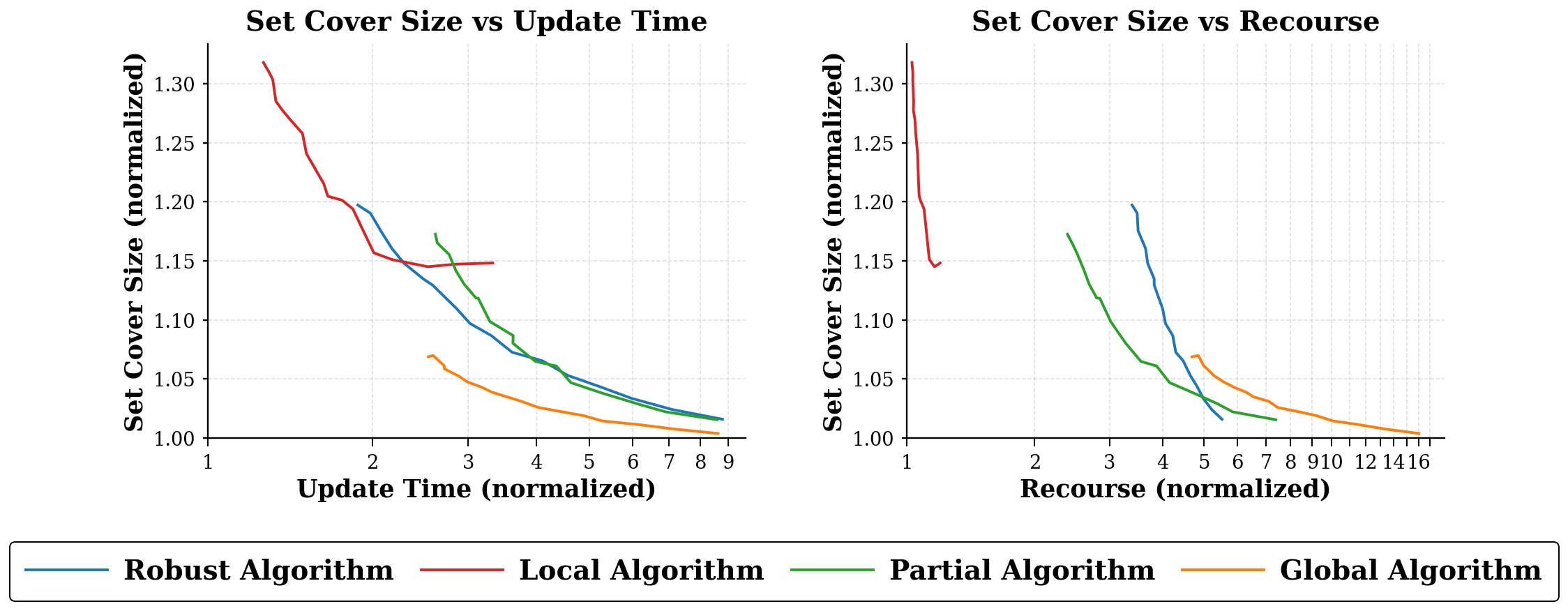
In the second step, to compare the four algorithms, we selected a representative for each by balancing the three quality metrics. While the optimal is application-dependent, we defined it as the value minimizing the objective function , where , and represent amortized set cover size, update time, and recourse, respectively. We chose this function to balance solution size against the other two metrics, which are strongly positively correlated. For each algorithm, we identified the minimizing per instance and used the median value across all instances as the “best” . The chosen ’s were 1.99, 1.9, 1.99 and 1.495 for the robust, local, partial and global algorithms respectively. Figure 2 presents the performance profiles comparing the four algorithms using these selected values.

The global algorithm achieves the smallest average set cover in 95% of instances (). The partial and robust algorithms follow, while the local algorithm generally yields the lowest-quality results. For amortized recourse, the hierarchy is roughly reversed: the local algorithm always performs best (100% at ), followed by the partial, robust, and global algorithms. Low recourse for the local algorithm is expected, as it maintains the solution by consistently “patching” it rather than triggering broader recomputations. Amortized update time reveals a more nuanced tradeoff. The local algorithm is generally the fastest, achieving the top result in 60% of instances. While the partial algorithm never achieves the fastest time (0% at ), it exhibits the steepest growth, indicating that it consistently remains near the best performance. Conversely, the robust algorithm is the fastest in one-third of instances but shows the least steep growth, failing to reach 100% even at very high values, suggesting significant overhead in several instances. The global algorithm’s performance lies between these two. For both efficiency metrics (update time and recourse), the values are significantly higher than those for the quality metric (size). This indicates that solution quality is much more stable across algorithms than efficiency, mirroring the observed influence of on each algorithm’s performance. To summarize, generally the local algorithm offers the highest efficiency, the global algorithm the highest quality, and the robust and partial algorithms offer a balanced middle ground. All numeric results are in Tables 3, 4, and 5.
6 Conclusion
This paper provides the first empirical study of the dynamic set cover problem, bridging the gap between theory and practice. We implemented and evaluated four greedy-based algorithms: a novel and simple one, alongside three simplifications of state-of-the-art theoretical designs modified to prioritize practical efficiency over asymptotic bounds. Our evaluations focused on three amortized metrics: set cover size as a measure of quality, and update time and recourse as measures of efficiency. We assessed the tradeoff between these metrics for each algorithm, followed by a comparative analysis of the four algorithms.
Future Work.
A natural extension would be a comprehensive comparison of the four algorithms against a naive baseline that recomputes the set cover from scratch at every update. While we attempted this over several weeks by waiving the 48-hour time limit, the extreme computational overhead restricted successful runs to only the smaller instances. Preliminary results suggest that our dynamic algorithms provide drastic efficiency gains while maintaining competitive solution quality; however, full-scale benchmarking on the larger instances is required to fully verify these results.
While this study focuses on the unweighted dynamic set cover problem for its accessible and intuitive presentation, a natural next step is the weighted version. In this variant, each set has a weight and the goal is to maintain a minimum-weight cover. In practice, the weighted implementation would not differ significantly, as it would use the same core algorithmic procedures as a black box to maintain the solution.
A further compelling direction is the implementation of theoretical primal-dual-based dynamic set cover algorithms designed for the low-frequency regime (). Evaluating their performance against the greedy-based algorithms presented here across all instance types (low-frequency and high-frequency) would clarify whether primal-dual approaches are indeed superior for low-frequency instances. Furthermore, such a comparison would help identify the practical transition point where greedy algorithms become the more effective choice.
References
- [1] Amir Abboud, Raghavendra Addanki, Fabrizio Grandoni, Debmalya Panigrahi, and Barna Saha. Dynamic set cover: improved algorithms and lower bounds. In Proceedings of the 51st Annual ACM SIGACT Symposium on Theory of Computing, pages 114–125, 2019. doi:10.1145/3313276.3316376.
- [2] Spyros Angelopoulos, Christoph Dürr, and Shendan Jin. Online maximum matching with recourse. J. Comb. Optim., 40(4):974–1007, 2020. doi:10.1007/s10878-020-00641-w.
- [3] Eugenio Angriman, Henning Meyerhenke, Christian Schulz, and Bora Uçar. Fully-dynamic weighted matching approximation in practice. In Michael Bender, John Gilbert, Bruce Hendrickson, and Blair D. Sullivan, editors, Proceedings of the 2021 SIAM Conference on Applied and Computational Discrete Algorithms, ACDA 2021, Virtual Conference, July 19-21, 2021, pages 32–44. SIAM, 2021. doi:10.1137/1.9781611976830.4.
- [4] Sepehr Assadi, Krzysztof Onak, Baruch Schieber, and Shay Solomon. Fully dynamic maximal independent set with sublinear update time. In Proceedings of the 50th Annual ACM SIGACT Symposium on Theory of Computing, STOC 2018, pages 815–826, New York, NY, USA, 2018. Association for Computing Machinery. doi:10.1145/3188745.3188922.
- [5] Sepehr Assadi and Shay Solomon. Fully Dynamic Set Cover via Hypergraph Maximal Matching: An Optimal Approximation Through a Local Approach. In 29th Annual European Symposium on Algorithms (ESA 2021), volume 204 of Leibniz International Proceedings in Informatics (LIPIcs), pages 8:1–8:18. Schloss Dagstuhl – Leibniz-Zentrum für Informatik, 2021. doi:10.4230/LIPIcs.ESA.2021.8.
- [6] Nikhil Bansal, Anupam Gupta, Ravishankar Krishnaswamy, Kirk Pruhs, Kevin Schewior, and Cliff Stein. A 2-Competitive Algorithm For Online Convex Optimization With Switching Costs. In Naveen Garg, Klaus Jansen, Anup Rao, and José D. P. Rolim, editors, Approximation, Randomization, and Combinatorial Optimization. Algorithms and Techniques (APPROX/RANDOM 2015), volume 40 of Leibniz International Proceedings in Informatics (LIPIcs), pages 96–109, Dagstuhl, Germany, 2015. Schloss Dagstuhl – Leibniz-Zentrum für Informatik. doi:10.4230/LIPIcs.APPROX-RANDOM.2015.96.
- [7] Austin R. Benson, Ravi Kumar, and Andrew Tomkins. A discrete choice model for subset selection. In Proceedings of the eleventh ACM International Conference on Web Search and Data Mining (WSDM). ACM, 2018.
- [8] Aaron Bernstein, Jacob Holm, and Eva Rotenberg. Online bipartite matching with amortized O replacements. J. ACM, 66(5), 2019. doi:10.1145/3344999.
- [9] Aaron Bernstein, Tsvi Kopelowitz, Seth Pettie, Ely Porat, and Clifford Stein. Simultaneously Load Balancing for Every p-norm, With Reassignments. In Christos H. Papadimitriou, editor, 8th Innovations in Theoretical Computer Science Conference (ITCS 2017), volume 67 of Leibniz International Proceedings in Informatics (LIPIcs), pages 51:1–51:14, Dagstuhl, Germany, 2017. Schloss Dagstuhl – Leibniz-Zentrum für Informatik. doi:10.4230/LIPIcs.ITCS.2017.51.
- [10] Sayan Bhattacharya, Ruoxu Cen, and Debmalya Panigrahi. Fully dynamic set cover: Worst-case recourse and update time, 2025. arXiv:2511.08485.
- [11] Sayan Bhattacharya, Deeparnab Chakrabarty, and Monika Henzinger. Deterministic fully dynamic approximate vertex cover and fractional matching in O amortized update time. In International Conference on Integer Programming and Combinatorial Optimization, pages 86–98. Springer, 2017. doi:10.1007/978-3-319-59250-3_8.
- [12] Sayan Bhattacharya, Monika Henzinger, and Giuseppe F Italiano. Design of dynamic algorithms via primal-dual method. In International Colloquium on Automata, Languages, and Programming, pages 206–218. Springer, 2015. doi:10.1007/978-3-662-47672-7_17.
- [13] Sayan Bhattacharya, Monika Henzinger, and Danupon Nanongkai. A new deterministic algorithm for dynamic set cover. In 2019 IEEE 60th Annual Symposium on Foundations of Computer Science (FOCS), pages 406–423. IEEE, 2019. doi:10.1109/FOCS.2019.00033.
- [14] Sayan Bhattacharya, Monika Henzinger, Danupon Nanongkai, and Xiaowei Wu. Dynamic set cover: Improved amortized and worst-case update time. In Proceedings of the 2021 ACM-SIAM Symposium on Discrete Algorithms (SODA), pages 2537–2549. SIAM, 2021. doi:10.1137/1.9781611976465.150.
- [15] Jannick Borowitz, Ernestine Großmann, and Christian Schulz. Engineering fully dynamic -orientation algorithms. In Jonathan W. Berry, David B. Shmoys, Lenore Cowen, and Uwe Naumann, editors, SIAM Conference on Applied and Computational Discrete Algorithms, ACDA 2023, Seattle, WA, USA, May 31 - June 2, 2023, pages 25–37. SIAM, 2023. doi:10.1137/1.9781611977714.3.
- [16] Jannick Borowitz, Ernestine Großmann, and Christian Schulz. Optimal neighborhood exploration for dynamic independent sets. In Rezaul Chowdhury, Jonathan W. Berry, Kathrin Hanauer, and Bin Ren, editors, Proceedings of the 27th Symposium on Algorithm Engineering and Experiments, ALENEX 2025, New Orleans, LA, USA, January 12-13, 2025, pages 1–14. SIAM, 2025. doi:10.1137/1.9781611978339.1.
- [17] Bartłomiej Bosek, Dariusz Leniowski, Piotr Sankowski, and Anna Zych-Pawlewicz. A tight bound for shortest augmenting paths on trees. Theor. Comput. Sci., 901(C):45–61, January 2022. doi:10.1016/j.tcs.2021.11.025.
- [18] Anton Bukov, Shay Solomon, and Tianyi Zhang. Nearly optimal dynamic set cover: Breaking the quadratic-in-f time barrier. In Yossi Azar and Debmalya Panigrahi, editors, Proceedings of the 2025 Annual ACM-SIAM Symposium on Discrete Algorithms, SODA 2025, New Orleans, LA, USA, January 12-15, 2025, pages 824–863. SIAM, 2025. doi:10.1137/1.9781611978322.24.
- [19] Keren Censor-Hillel, Elad Haramaty, and Zohar Karnin. Optimal dynamic distributed mis. In Proceedings of the 2016 ACM Symposium on Principles of Distributed Computing, PODC ’16, pages 217–226, New York, NY, USA, 2016. Association for Computing Machinery. doi:10.1145/2933057.2933083.
- [20] K. Chaudhuri, C. Daskalakis, R. D. Kleinberg, and H. Lin. Online bipartite perfect matching with augmentations. In IEEE INFOCOM 2009, pages 1044–1052, 2009. doi:10.1109/INFCOM.2009.5062016.
- [21] V. Chvatal. A greedy heuristic for the set-covering problem. Mathematics of Operations Research, 4(3):233–235, 1979. doi:10.1287/MOOR.4.3.233.
- [22] Graham Cormode, Howard Karloff, and Anthony Wirth. Set cover algorithms for very large datasets. In Proceedings of the 19th ACM International Conference on Information and Knowledge Management, CIKM ’10, pages 479–488, New York, NY, USA, 2010. Association for Computing Machinery. doi:10.1145/1871437.1871501.
- [23] Timothy A. Davis and Yifan Hu. The university of florida sparse matrix collection. ACM Trans. Math. Softw., 38(1), 2011. doi:10.1145/2049662.2049663.
- [24] Irit Dinur and David Steurer. Analytical approach to parallel repetition. In Proceedings of the forty-sixth annual ACM symposium on Theory of computing, pages 624–633, 2014. doi:10.1145/2591796.2591884.
- [25] Elizabeth D. Dolan and Jorge J. Moré. Benchmarking optimization software with performance profiles, 2004. arXiv:cs/0102001.
- [26] Chao Gao, Xin Yao, Thomas Weise, and Jinlong Li. An efficient local search heuristic with row weighting for the unicost set covering problem. European Journal of Operational Research, 246(3):750–761, 2015. doi:10.1016/j.ejor.2015.05.038.
- [27] Gramoz Goranci, Monika Henzinger, Dariusz Leniowski, Christian Schulz, and Alexander Svozil. Fully dynamic k-center clustering in low dimensional metrics. In Martin Farach-Colton and Sabine Storandt, editors, Proceedings of the 23rd Symposium on Algorithm Engineering and Experiments, ALENEX 2021, Virtual Conference, January 10-11, 2021, pages 143–153. SIAM, 2021. doi:10.1137/1.9781611976472.11.
- [28] Ernestine Großmann, Henrik Reinstädtler, Eva Rotenberg, Christian Schulz, Ivor van der Hoog, and Juliette Vlieghe. From theory to practice: Engineering approximation algorithms for dynamic orientation. In Anne Benoit, Haim Kaplan, Sebastian Wild, and Grzegorz Herman, editors, 33rd Annual European Symposium on Algorithms, ESA 2025, Warsaw, Poland, September 15-17, 2025, volume 351 of LIPIcs, pages 65:1–65:18. Schloss Dagstuhl – Leibniz-Zentrum für Informatik, 2025. doi:10.4230/LIPIcs.ESA.2025.65.
- [29] Ernestine Großmann, Henrik Reinstädtler, Christian Schulz, and Fabian Walliser. Engineering fully dynamic exact -orientation algorithms. In Rezaul Chowdhury, Jonathan W. Berry, Kathrin Hanauer, and Bin Ren, editors, Proceedings of the 27th Symposium on Algorithm Engineering and Experiments, ALENEX 2025, New Orleans, LA, USA, January 12-13, 2025, pages 15–28. SIAM, 2025. doi:10.1137/1.9781611978339.2.
- [30] Edward F. Grove, Ming-Yang Kao, P. Krishnan, and Jeffrey Scott Vitter. Online perfect matching and mobile computing. In Proceedings of the 4th International Workshop on Algorithms and Data Structures, WADS ’95, pages 194–205, Berlin, Heidelberg, 1995. Springer-Verlag. doi:10.1007/3-540-60220-8_62.
- [31] Albert Gu, Anupam Gupta, and Amit Kumar. The power of deferral: maintaining a constant-competitive steiner tree online. In Proceedings of the Forty-Fifth Annual ACM Symposium on Theory of Computing, STOC ’13, pages 525–534, New York, NY, USA, 2013. Association for Computing Machinery. doi:10.1145/2488608.2488674.
- [32] Anupam Gupta, Ravishankar Krishnaswamy, Amit Kumar, and Debmalya Panigrahi. Online and dynamic algorithms for set cover. In Proceedings of the 49th Annual ACM SIGACT Symposium on Theory of Computing, pages 537–550, 2017. doi:10.1145/3055399.3055493.
- [33] Anupam Gupta and Amit Kumar. Online steiner tree with deletions. In Proceedings of the Twenty-Fifth Annual ACM-SIAM Symposium on Discrete Algorithms, SODA ’14, pages 455–467, USA, 2014. Society for Industrial and Applied Mathematics. doi:10.1137/1.9781611973402.34.
- [34] Anupam Gupta, Amit Kumar, and Cliff Stein. Maintaining assignments online: matching, scheduling, and flows. In Proceedings of the Twenty-Fifth Annual ACM-SIAM Symposium on Discrete Algorithms, SODA ’14, pages 468–479, USA, 2014. Society for Industrial and Applied Mathematics. doi:10.1137/1.9781611973402.35.
- [35] Kathrin Hanauer, Monika Henzinger, Lara Ost, and Stefan Schmid. Dynamic demand-aware link scheduling for reconfigurable datacenters. In IEEE INFOCOM 2023 - IEEE Conference on Computer Communications, New York City, NY, USA, May 17-20, 2023, pages 1–10. IEEE, 2023. doi:10.1109/INFOCOM53939.2023.10229050.
- [36] Kathrin Hanauer, Monika Henzinger, and Christian Schulz. Faster fully dynamic transitive closure in practice. In Simone Faro and Domenico Cantone, editors, 18th International Symposium on Experimental Algorithms, SEA 2020, Catania, Italy, June 16-18, 2020, volume 160 of LIPIcs, pages 14:1–14:14. Schloss Dagstuhl – Leibniz-Zentrum für Informatik, 2020. doi:10.4230/LIPIcs.SEA.2020.14.
- [37] Kathrin Hanauer, Monika Henzinger, and Christian Schulz. Fully dynamic single-source reachability in practice: An experimental study. In Guy E. Blelloch and Irene Finocchi, editors, Proceedings of the 22nd Symposium on Algorithm Engineering and Experiments, ALENEX 2020, Salt Lake City, UT, USA, January 5-6, 2020, pages 106–119. SIAM, 2020. doi:10.1137/1.9781611976007.9.
- [38] Kathrin Hanauer, Monika Henzinger, and Christian Schulz. Recent advances in fully dynamic graph algorithms - A quick reference guide. ACM J. Exp. Algorithmics, 27:1.11:1–1.11:45, 2022. doi:10.1145/3555806.
- [39] Monika Henzinger, Shahbaz Khan, Richard D. Paul, and Christian Schulz. Dynamic matching algorithms in practice. In Fabrizio Grandoni, Grzegorz Herman, and Peter Sanders, editors, 28th Annual European Symposium on Algorithms, ESA 2020, Pisa, Italy (Virtual Conference), September 7-9, 2020, volume 173 of LIPIcs, pages 58:1–58:20. Schloss Dagstuhl – Leibniz-Zentrum für Informatik, 2020. doi:10.4230/LIPIcs.ESA.2020.58.
- [40] Monika Henzinger, Alexander Noe, and Christian Schulz. Practical fully dynamic minimum cut algorithms. In Cynthia A. Phillips and Bettina Speckmann, editors, Proceedings of the 24th Symposium on Algorithm Engineering and Experiments, ALENEX 2022, Alexandria, VA, USA, January 9-10, 2022, pages 13–26. SIAM, 2022. doi:10.1137/1.9781611977042.2.
- [41] David S. Johnson. Approximation algorithms for combinatorial problems. Journal of Computer and System Sciences, 9(3):256–278, 1974. doi:10.1016/S0022-0000(74)80044-9.
- [42] Subhash Khot and Oded Regev. Vertex cover might be hard to approximate to within . Journal of Computer and System Sciences, 74(3):335–349, 2008.
- [43] L. Lovász. On the ratio of optimal integral and fractional covers. Discrete Mathematics, 13(4):383–390, 1975. doi:10.1016/0012-365X(75)90058-8.
- [44] Chuan Luo, Wenqian Xing, Shaowei Cai, and Chunming Hu. NuSC: An effective local search algorithm for solving the set covering problem. IEEE Transactions on Cybernetics, 54(3):1403–1416, 2024. doi:10.1109/TCYB.2022.3199147.
- [45] Nicole Megow, Martin Skutella, José Verschae, and Andreas Wiese. The power of recourse for online MST and TSP. SIAM Journal on Computing, 45(3):859–880, 2016. doi:10.1137/130917703.
- [46] Jianmo Ni, Jiacheng Li, and Julian McAuley. Justifying recommendations using distantly-labeled reviews and fine-grained aspects. In Proceedings of the 2019 Conference on Empirical Methods in Natural Language Processing and the 9th International Joint Conference on Natural Language Processing (EMNLP-IJCNLP), pages 188–197, 2019. doi:10.18653/V1/D19-1018.
- [47] Barna Saha and Lise Getoor. On maximum coverage in the streaming model & application to multi-topic blog-watch. In Proceedings of the SIAM International Conference on Data Mining, SDM 2009, April 30 - May 2, 2009, Sparks, Nevada, USA, pages 697–708. SIAM, 2009. doi:10.1137/1.9781611972795.60.
- [48] Noam Solomon and Shay Solomon. A Generalized Matching Reconfiguration Problem. In James R. Lee, editor, 12th Innovations in Theoretical Computer Science Conference (ITCS 2021), volume 185 of Leibniz International Proceedings in Informatics (LIPIcs), pages 57:1–57:20, Dagstuhl, Germany, 2021. Schloss Dagstuhl – Leibniz-Zentrum für Informatik. doi:10.4230/LIPIcs.ITCS.2021.57.
- [49] Shay Solomon and Amitai Uzrad. Dynamic -Approximation Algorithms for Minimum Set Cover and Dominating Set. In Proceedings of the 55th Annual ACM Symposium on Theory of Computing, pages 1187–1200, 2023. doi:10.1145/3564246.3585211.
- [50] Shay Solomon and Amitai Uzrad. Dynamic set cover with worst-case recourse, 2025. arXiv:2511.07354.
- [51] Shay Solomon, Amitai Uzrad, and Tianyi Zhang. A lossless deamortization for dynamic greedy set cover. In 2024 IEEE 65th Annual Symposium on Foundations of Computer Science (FOCS), pages 264–290, 2024. doi:10.1109/FOCS61266.2024.00025.
- [52] Yiyuan Wang, Shiwei Pan, Sameh Al-Shihabi, Junping Zhou, Nan Yang, and Minghao Yin. An improved configuration checking-based algorithm for the unicost set covering problem. European Journal of Operational Research, 294(2):476–491, 2021. doi:10.1016/j.ejor.2021.02.015.
- [53] David P Williamson and David B Shmoys. The design of approximation algorithms. Cambridge university press, 2011.
- [54] Belma Yelbay, Ş. İlker Birbil, and Kerem Bülbül. The set covering problem revisited: An empirical study of the value of dual information, 2015. doi:10.3934/jimo.2015.11.575.
Appendix A Appendix
![[Uncaptioned image]](figpp1.png)
![[Uncaptioned image]](figpp2.png)
![[Uncaptioned image]](figpp3.png)

| Ins. | (ns) | (ns) | (ns) | (ns) | ||||||||||||
|---|---|---|---|---|---|---|---|---|---|---|---|---|---|---|---|---|
| 1 | 5082 | 254 | 31022 | 969 | 287.753 | 5439.58 | 1.9264 | 229.997 | 5367.95 | 0.9976 | 229.973 | 23606.32 | 2.0256 | 229.989 | 17360.48 | 2.2735 |
| 2 | 6318 | 315 | 15905 | 1837 | 5.3107 | 4432988.0 | 0.7822 | 5.8957 | 295395.6 | 0.0332 | 5.1955 | 451731.4 | 0.082 | 4.4395 | 100355.76 | 0.132 |
| 3 | 9858 | 492 | 10595 | 4928 | 129.646 | 7225.73 | 1.0742 | 130.12 | 3672.21 | 0.3518 | 125.407 | 11980.24 | 1.016 | 117.572 | 14571.88 | 2.1319 |
| 4 | 12442 | 622 | 22687 | 64 | 388.074 | 4709.44 | 1.5224 | 423.81 | 3070.41 | 0.664 | 372.093 | 9170.11 | 1.3411 | 347.446 | 16667.04 | 2.3088 |
| 5 | 21162 | 1058 | 10581 | 1711 | 4.8038 | 597014.6 | 0.1294 | 5.5951 | 22575.16 | 0.0076 | 4.9958 | 27667.5 | 0.0248 | 4.5228 | 13734.0 | 0.0546 |
| 6 | 21210 | 1060 | 10605 | 147 | 493.559 | 58525.96 | 0.5902 | 402.969 | 13249.22 | 0.4395 | 402.346 | 22153.32 | 0.5204 | 400.905 | 13959.2 | 0.6058 |
| 7 | 21548 | 1077 | 10774 | 11 | 481.57 | 4013.7 | 1.4498 | 515.562 | 3626.16 | 0.5787 | 446.808 | 9093.77 | 1.4478 | 412.166 | 12453.46 | 2.5068 |
| 8 | 21696 | 1084 | 10848 | 723 | 53.3009 | 116051.8 | 0.4747 | 55.8195 | 33474.22 | 0.0745 | 54.2873 | 62388.62 | 0.2895 | 49.6107 | 38395.18 | 0.7263 |
| 9 | 22794 | 1139 | 11397 | 25 | 266.566 | 7844.93 | 1.5366 | 302.59 | 5229.61 | 0.4943 | 262.863 | 11901.06 | 0.9913 | 232.73 | 14964.96 | 1.9488 |
| 10 | 23476 | 1173 | 11738 | 10 | 492.033 | 3437.06 | 1.4334 | 527.189 | 2804.5 | 0.6025 | 462.834 | 8045.11 | 1.4809 | 422.81 | 11600.02 | 2.4291 |
| 11 | 23580 | 1179 | 11790 | 120 | 363.083 | 4192.15 | 0.9394 | 381.919 | 3616.16 | 0.4694 | 337.913 | 7705.03 | 0.9617 | 325.289 | 10764.32 | 1.5578 |
| 12 | 24010 | 1200 | 12005 | 50 | 141.853 | 9535.68 | 0.8262 | 146.363 | 7709.88 | 0.2482 | 140.207 | 13628.18 | 0.5286 | 134.122 | 11246.14 | 0.9512 |
| 13 | 24656 | 1232 | 12328 | 121 | 251.145 | 16694.0 | 1.4178 | 321.063 | 10478.06 | 0.4169 | 247.344 | 22044.62 | 1.0903 | 222.794 | 24964.76 | 1.978 |
| 14 | 24942 | 1247 | 872622 | 75355 | 81.1309 | 17736340 | 0.9063 | 92.955 | 3196086.0 | 0.1148 | 82.2677 | 4873080.0 | 0.309 | 75.4089 | 1843784.0 | 0.6323 |
| 15 | 25196 | 1259 | 12598 | 33 | 185.937 | 7710.13 | 1.2108 | 219.402 | 6284.92 | 0.4707 | 187.785 | 12027.92 | 0.9252 | 166.901 | 14449.38 | 1.9537 |
| 16 | 26628 | 1331 | 13332 | 2265 | 378.416 | 11178.3 | 0.6427 | 400.065 | 8507.19 | 0.2609 | 371.537 | 15223.34 | 0.5086 | 364.064 | 9659.76 | 0.812 |
| 17 | 26712 | 1335 | 13356 | 102 | 325.733 | 6319.12 | 1.053 | 342.499 | 3667.42 | 0.4701 | 301.547 | 9147.24 | 1.1082 | 287.222 | 10794.8 | 1.6548 |
| 18 | 27070 | 1353 | 13535 | 45 | 279.234 | 16505.0 | 1.5217 | 285.45 | 10686.1 | 0.5386 | 256.446 | 26253.96 | 1.1461 | 233.179 | 32938.62 | 2.3593 |
| 19 | 27382 | 1369 | 13682 | 16 | 38.785 | 60562.08 | 0.2975 | 42.0452 | 4346.54 | 0.0195 | 41.0081 | 10675.36 | 0.0638 | 39.4657 | 7348.85 | 0.1196 |
| 20 | 27930 | 1396 | 13965 | 81 | 53.7755 | 60389.92 | 0.9726 | 69.073 | 27803.2 | 0.227 | 56.5894 | 37932.16 | 0.352 | 49.4463 | 27013.06 | 0.7986 |
| 21 | 27984 | 1399 | 13992 | 71 | 110.164 | 23130.3 | 0.6693 | 110.897 | 15164.62 | 0.167 | 111.56 | 24851.78 | 0.6156 | 94.8106 | 19204.4 | 1.3084 |
| 22 | 28000 | 1400 | 14000 | 294 | 138.933 | 117946.0 | 1.7516 | 191.976 | 63926.84 | 0.1455 | 151.35 | 129075.0 | 0.4919 | 123.422 | 79639.46 | 1.0205 |
| 23 | 28428 | 1421 | 14214 | 23 | 218.824 | 8120.68 | 1.0419 | 240.805 | 7803.96 | 0.5428 | 209.888 | 16043.5 | 0.8477 | 197.064 | 13090.64 | 1.2028 |
| 24 | 28680 | 1434 | 14340 | 7229 | 121.762 | 661128.8 | 0.9397 | 133.866 | 720395.2 | 0.099 | 125.582 | 1190086.0 | 0.2348 | 118.329 | 96371.52 | 0.3708 |
| 25 | 29644 | 1482 | 14822 | 50 | 74.034 | 41130.12 | 0.705 | 76.7424 | 17677.26 | 0.1218 | 72.958 | 36337.02 | 0.413 | 68.5249 | 27149.96 | 1.0737 |
| 26 | 30480 | 1524 | 72600 | 20 | 143.352 | 68947.54 | 0.0974 | 141.252 | 8486.27 | 0.0736 | 141.086 | 26988.5 | 0.1085 | 141.072 | 44504.42 | 0.2437 |
| 27 | 30874 | 1543 | 19321 | 63 | 446.712 | 7778.8 | 1.5377 | 543.375 | 6081.94 | 0.5825 | 463.415 | 13707.8 | 1.1299 | 399.93 | 19673.24 | 2.2271 |
| 28 | 30898 | 1544 | 15449 | 243 | 30.6138 | 186241.6 | 0.446 | 36.5083 | 39865.64 | 0.0538 | 31.5938 | 56368.06 | 0.1527 | 28.1611 | 24032.02 | 0.3232 |
| 29 | 32092 | 1604 | 16706 | 360 | 600.745 | 7483.63 | 0.853 | 598.463 | 5605.71 | 0.3616 | 570.373 | 13116.2 | 0.8328 | 546.345 | 16094.64 | 1.4241 |
| 30 | 32292 | 1614 | 16146 | 89 | 62.9686 | 53537.52 | 0.6633 | 71.9663 | 20541.48 | 0.1279 | 64.2677 | 37139.38 | 0.3511 | 58.7613 | 30429.48 | 0.9428 |
| 31 | 33566 | 1678 | 16783 | 14672 | 4.5682 | 6224774.0 | 0.1951 | 3.3493 | 208021.8 | 0.0162 | 4.8707 | 421492.8 | 0.0243 | 3.9648 | 42573.1 | 0.0275 |
| 32 | 34444 | 1722 | 17222 | 19 | 305.2 | 7201.02 | 0.9005 | 401.459 | 5170.08 | 0.4385 | 316.504 | 9731.86 | 0.8177 | 283.107 | 11925.94 | 1.4998 |
| 33 | 34722 | 1736 | 17361 | 360 | 54.6294 | 72249.52 | 0.4594 | 54.4614 | 19281.2 | 0.0552 | 54.5105 | 32236.98 | 0.268 | 49.874 | 22617.64 | 0.7517 |
| 34 | 40000 | 2000 | 20000 | 29 | 232.307 | 28545.6 | 2.0232 | 300.394 | 17879.46 | 0.4068 | 232.741 | 27688.12 | 0.7719 | 200.726 | 37413.16 | 1.7052 |
| 35 | 41792 | 2089 | 20896 | 12 | 996.075 | 6902.75 | 1.8538 | 1148.0 | 7179.37 | 0.6057 | 999.954 | 15643.24 | 1.4432 | 893.392 | 21968.76 | 2.8161 |
| 36 | 42072 | 2103 | 21036 | 28 | 800.972 | 10293.52 | 1.6462 | 895.052 | 8660.18 | 0.5157 | 794.798 | 19269.38 | 1.2963 | 697.87 | 27277.34 | 2.3827 |
| 37 | 45120 | 2256 | 22560 | 112 | 123.345 | 32152.92 | 0.4948 | 128.751 | 23294.42 | 0.1341 | 120.369 | 32639.78 | 0.4695 | 113.73 | 22213.24 | 0.8515 |
| 38 | 45390 | 2269 | 22695 | 108 | 131.388 | 49422.1 | 1.5047 | 168.574 | 31148.32 | 0.3229 | 137.817 | 47887.34 | 0.6042 | 117.817 | 36055.26 | 1.2281 |
| 39 | 46824 | 2341 | 23412 | 15 | 499.27 | 6499.2 | 1.4433 | 502.693 | 6838.26 | 0.7461 | 461.733 | 12886.74 | 1.2276 | 415.601 | 17960.76 | 2.2906 |
| 40 | 47120 | 2356 | 23560 | 21 | 268.884 | 13449.04 | 1.4885 | 322.396 | 11399.88 | 0.534 | 251.649 | 20568.96 | 0.938 | 228.249 | 24901.46 | 1.8933 |
| Ins. | (ns) | (ns) | (ns) | (ns) | ||||||||||||
|---|---|---|---|---|---|---|---|---|---|---|---|---|---|---|---|---|
| 41 | 49082 | 2454 | 27240 | 562 | 625.902 | 9307.64 | 0.6807 | 660.548 | 6924.21 | 0.2466 | 617.088 | 11296.98 | 0.5046 | 595.109 | 11585.72 | 0.8174 |
| 42 | 49684 | 2484 | 24842 | 181 | 815.195 | 3815.55 | 1.0488 | 769.687 | 3039.94 | 0.4521 | 746.872 | 8502.3 | 1.2439 | 711.249 | 14896.42 | 2.4125 |
| 43 | 50374 | 2518 | 25187 | 22767 | 174.51 | 43786.98 | 0.2217 | 206.162 | 3400.64 | 0.0931 | 180.249 | 7298.35 | 0.1745 | 174.105 | 8408.98 | 0.2884 |
| 44 | 55386 | 2769 | 67593 | 15 | 1399.49 | 5260.27 | 1.9145 | 2337.1 | 3612.38 | 0.8711 | 1412.34 | 10485.92 | 1.5539 | 1200.35 | 21386.36 | 2.6747 |
| 45 | 58134 | 2906 | 29067 | 345 | 314.489 | 68813.42 | 1.1207 | 335.838 | 34598.06 | 0.0785 | 318.418 | 84512.86 | 0.4671 | 290.921 | 41045.6 | 0.8276 |
| 46 | 58564 | 2928 | 29282 | 18 | 686.571 | 7359.38 | 1.1924 | 640.005 | 6167.8 | 0.6086 | 635.622 | 15335.74 | 1.252 | 583.915 | 21675.04 | 2.3749 |
| 47 | 59840 | 2992 | 29920 | 181 | 319.474 | 156509.8 | 0.4433 | 294.381 | 26572.56 | 0.1382 | 290.356 | 58197.24 | 0.3901 | 288.642 | 40787.36 | 0.8214 |
| 48 | 59914 | 2995 | 29957 | 154 | 452.936 | 45564.02 | 1.3872 | 481.115 | 28505.94 | 0.3979 | 428.234 | 63750.36 | 0.9428 | 386.377 | 62983.1 | 1.9834 |
| 49 | 59990 | 2999 | 29995 | 8 | 719.544 | 3548.32 | 0.9202 | 744.789 | 3311.07 | 0.678 | 647.689 | 8380.51 | 1.306 | 573.906 | 14355.38 | 2.4728 |
| 50 | 60324 | 3016 | 27944 | 120 | 372.29 | 20323.88 | 1.4106 | 473.213 | 14440.36 | 0.2528 | 382.513 | 27533.26 | 0.5279 | 344.009 | 19768.64 | 1.1143 |
| 51 | 61596 | 3079 | 30798 | 15054 | 1085.05 | 2536456.0 | 0.9414 | 1465.63 | 20733.58 | 0.4965 | 1074.85 | 34748.68 | 0.8537 | 925.56 | 14836.0 | 1.497 |
| 52 | 65538 | 3276 | 32769 | 73 | 611.819 | 8467.07 | 0.983 | 649.748 | 5053.44 | 0.2886 | 623.542 | 12727.86 | 0.7041 | 553.48 | 19463.96 | 1.3422 |
| 53 | 69840 | 3492 | 34920 | 438 | 93.2377 | 177874.0 | 0.4484 | 98.4801 | 52920.5 | 0.0541 | 96.4026 | 105585.8 | 0.2169 | 87.2432 | 55472.94 | 0.6411 |
| 54 | 72000 | 3600 | 36000 | 519 | 83.1629 | 677449.4 | 0.7467 | 98.2479 | 190210.8 | 0.0805 | 83.2803 | 494395.6 | 0.2549 | 74.4111 | 167191.8 | 0.6039 |
| 55 | 72834 | 3641 | 36417 | 204 | 92.1224 | 143161.6 | 0.5019 | 94.7967 | 49827.3 | 0.098 | 93.3368 | 102867.6 | 0.3338 | 84.0223 | 52800.12 | 0.8015 |
| 56 | 72882 | 3644 | 36441 | 21 | 430.192 | 9133.73 | 1.3889 | 550.951 | 7180.16 | 0.3853 | 427.316 | 16499.78 | 0.9336 | 386.526 | 19152.56 | 1.5548 |
| 57 | 75524 | 3776 | 37762 | 42 | 230.075 | 21419.74 | 1.0404 | 228.548 | 11830.38 | 0.2012 | 228.978 | 27324.56 | 0.5877 | 210.938 | 24545.64 | 1.2327 |
| 58 | 76830 | 3841 | 38415 | 25 | 370.753 | 14288.6 | 1.353 | 384.167 | 12169.92 | 0.8967 | 372.303 | 24290.32 | 1.1529 | 331.347 | 26618.62 | 1.6782 |
| 59 | 77488 | 3874 | 38744 | 126 | 338.292 | 24759.72 | 1.2871 | 351.147 | 20005.28 | 0.3723 | 312.861 | 35750.32 | 0.7343 | 285.503 | 31002.66 | 1.6101 |
| 60 | 80432 | 4021 | 40216 | 20024 | 1416.94 | 2139940.0 | 0.7985 | 1936.55 | 14913.24 | 0.499 | 1401.5 | 24006.06 | 0.8433 | 1210.61 | 22775.22 | 1.5658 |
| 61 | 91816 | 4590 | 59498 | 155 | 2119.28 | 11169.46 | 1.2688 | 1997.2 | 14480.72 | 0.6008 | 1832.86 | 28294.0 | 1.3832 | 1790.24 | 38953.84 | 1.9314 |
| 62 | 93670 | 4683 | 46835 | 145 | 280.704 | 41693.28 | 0.6525 | 293.8 | 34259.32 | 0.1286 | 275.506 | 56622.5 | 0.6023 | 253.137 | 52783.56 | 1.6431 |
| 63 | 98304 | 4915 | 49152 | 39 | 322.384 | 36298.34 | 1.0097 | 382.34 | 30151.68 | 0.2108 | 335.429 | 48212.82 | 0.5105 | 292.848 | 52119.24 | 1.3681 |
| 64 | 99332 | 4966 | 49666 | 13 | 1411.68 | 11181.86 | 1.6046 | 1356.6 | 12454.44 | 0.9019 | 1205.61 | 24501.94 | 1.5696 | 1127.74 | 36975.72 | 2.6239 |
| 65 | 100000 | 5000 | 50000 | 56 | 1429.04 | 26476.1 | 1.8846 | 1765.89 | 31928.68 | 0.3916 | 1532.19 | 54616.56 | 1.0679 | 1254.71 | 64572.92 | 2.3124 |
| 66 | 103986 | 5199 | 51993 | 23 | 2244.17 | 5764.94 | 1.2888 | 2092.49 | 4778.71 | 0.7251 | 1936.21 | 13221.28 | 1.23 | 1857.95 | 24396.42 | 2.0975 |
| 67 | 108038 | 5401 | 54019 | 1426 | 608.248 | 10551.14 | 0.8116 | 702.365 | 8952.75 | 0.2926 | 612.864 | 17900.26 | 0.7101 | 551.865 | 28306.18 | 1.8233 |
| 68 | 109740 | 5487 | 54870 | 276 | 246.101 | 40571.08 | 0.7167 | 313.446 | 19827.44 | 0.2365 | 255.068 | 58393.98 | 0.5453 | 218.236 | 39506.86 | 1.2134 |
| 69 | 110642 | 5532 | 65536 | 17998 | 821.432 | 59605.04 | 0.2977 | 851.236 | 58062.8 | 0.1307 | 817.135 | 149445.6 | 0.2035 | 808.524 | 28235.44 | 0.278 |
| 70 | 120000 | 6000 | 60000 | 36 | 2507.76 | 10453.78 | 1.7553 | 2940.96 | 11179.58 | 0.5699 | 2549.41 | 24881.2 | 1.3139 | 2208.49 | 40767.56 | 2.5131 |
| 71 | 121480 | 6074 | 60740 | 63 | 476.257 | 21366.28 | 1.0353 | 583.219 | 20764.12 | 0.3997 | 502.888 | 37234.38 | 0.6978 | 441.649 | 48738.72 | 1.678 |
| 72 | 124848 | 6242 | 62424 | 44 | 462.051 | 17984.1 | 0.6377 | 440.016 | 12976.92 | 0.2227 | 459.695 | 35121.7 | 0.5946 | 424.831 | 34267.44 | 1.4813 |
| 73 | 130050 | 6502 | 65025 | 25 | 1680.17 | 11666.68 | 1.0524 | 1638.76 | 8729.21 | 0.4631 | 1576.03 | 30429.82 | 1.282 | 1459.01 | 40958.36 | 2.2551 |
| 74 | 131072 | 6553 | 147266 | 9 | 2403.97 | 6650.09 | 1.4349 | 2600.77 | 6507.06 | 0.5834 | 2436.47 | 18177.28 | 1.3217 | 1958.68 | 46429.1 | 2.8214 |
| 75 | 132254 | 6612 | 66127 | 27 | 649.921 | 16117.12 | 1.5108 | 734.344 | 14118.62 | 0.7324 | 645.14 | 29710.46 | 0.9834 | 571.841 | 37382.3 | 1.9701 |
| 76 | 134048 | 6702 | 67024 | 37 | 695.539 | 29899.42 | 1.8317 | 866.885 | 25726.96 | 0.3843 | 687.702 | 41471.36 | 0.7647 | 585.256 | 55100.22 | 1.7964 |
| 77 | 134346 | 6717 | 67173 | 89 | 1825.25 | 20281.18 | 0.7654 | 1763.83 | 39187.32 | 0.556 | 1669.66 | 64928.06 | 0.6576 | 1627.93 | 32812.94 | 0.8759 |
| 78 | 136242 | 6812 | 68121 | 68121 | 641.157 | 58528.46 | 1.428 | 712.806 | 53892.58 | 0.8876 | 644.97 | 80256.3 | 1.0534 | 569.416 | 52729.84 | 1.7393 |
| 79 | 138470 | 6923 | 132402 | 12 | 2210.99 | 10213.44 | 1.8489 | 2293.49 | 9309.22 | 0.9065 | 1922.55 | 24556.08 | 1.5748 | 1716.88 | 50530.36 | 2.9107 |
| 80 | 141312 | 7065 | 70656 | 33 | 690.723 | 17319.5 | 1.4105 | 793.481 | 15555.84 | 0.5777 | 689.886 | 35562.68 | 0.8948 | 607.741 | 40741.6 | 1.8693 |
| Ins. | (ns) | (ns) | (ns) | (ns) | ||||||||||||
|---|---|---|---|---|---|---|---|---|---|---|---|---|---|---|---|---|
| 81 | 143010 | 7150 | 71505 | 345 | 406.119 | 86216.38 | 0.5872 | 422.233 | 41982.32 | 0.085 | 413.092 | 101455.2 | 0.428 | 365.102 | 75259.84 | 1.2086 |
| 82 | 148124 | 7406 | 74062 | 565 | 1159.82 | 13134.08 | 1.0639 | 1449.92 | 15502.24 | 0.3562 | 1174.96 | 32477.86 | 0.8353 | 1047.17 | 33857.38 | 1.7232 |
| 83 | 148208 | 7410 | 74104 | 271 | 3087.19 | 4854.94 | 1.5042 | 3737.19 | 4993.87 | 0.8528 | 2760.14 | 13686.02 | 1.4677 | 2597.86 | 27076.82 | 2.3288 |
| 84 | 149504 | 7475 | 74752 | 55 | 1369.94 | 8009.24 | 0.7135 | 1507.18 | 5451.76 | 0.3946 | 1256.91 | 15235.08 | 0.8653 | 1224.47 | 28892.46 | 1.7676 |
| 85 | 165308 | 8265 | 82654 | 11 | 2232.74 | 12981.92 | 1.0016 | 2128.83 | 20326.32 | 0.4931 | 2082.32 | 33490.1 | 1.2002 | 1906.97 | 49537.1 | 2.11 |
| 86 | 171246 | 8562 | 85623 | 145 | 1297.64 | 40428.1 | 1.0856 | 1447.73 | 60738.0 | 0.1638 | 1317.96 | 114105.2 | 0.5942 | 1187.86 | 75020.18 | 1.1062 |
| 87 | 175608 | 8780 | 87804 | 132 | 392.276 | 58128.84 | 0.5105 | 405.038 | 73533.52 | 0.078 | 391.8 | 100322.66 | 0.3123 | 372.918 | 69685.8 | 1.0038 |
| 88 | 178800 | 8940 | 89400 | 13 | 1513.22 | 17057.12 | 1.429 | 1589.41 | 30912.8 | 0.6426 | 1402.72 | 47089.74 | 1.1074 | 1226.39 | 59792.66 | 1.9877 |
| 89 | 180898 | 9044 | 90449 | 42 | 422.812 | 40805.1 | 0.5694 | 453.53 | 49843.22 | 0.1519 | 429.618 | 90117.7 | 0.3927 | 399.007 | 70889.02 | 1.1179 |
| 90 | 202984 | 10149 | 101492 | 31 | 1421.63 | 24747.46 | 1.0418 | 1621.42 | 40231.24 | 0.3821 | 1372.5 | 66061.54 | 0.9159 | 1248.71 | 76300.0 | 1.9331 |
| 91 | 204316 | 10215 | 102158 | 10 | 4840.37 | 18862.28 | 1.5964 | 5327.28 | 32273.54 | 0.5937 | 4686.8 | 53719.0 | 1.4096 | 4230.74 | 71840.14 | 2.5552 |
| 92 | 226152 | 11307 | 113076 | 7031 | 2006.37 | 27508.56 | 1.2961 | 2040.4 | 35498.72 | 0.4657 | 1868.42 | 98471.7 | 1.1365 | 1689.57 | 79854.74 | 2.3881 |
| 93 | 233670 | 11683 | 116835 | 114190 | 224.66 | 59180.78 | 0.0748 | 223.176 | 7584.04 | 0.0228 | 223.176 | 16260.32 | 0.0492 | 223.176 | 32563.5 | 0.0578 |
| 94 | 306452 | 15322 | 153226 | 5776 | 2555.71 | 30755.04 | 1.2261 | 2643.92 | 45486.6 | 0.4635 | 2375.3 | 126643.2 | 1.1055 | 2157.53 | 109772.8 | 2.484 |
| 95 | 307492 | 15374 | 153746 | 99 | 533.182 | 60106.94 | 0.6453 | 608.962 | 51563.38 | 0.1476 | 535.917 | 136503.0 | 0.4574 | 478.42 | 75068.42 | 1.1144 |
| 96 | 314928 | 15746 | 157464 | 27 | 1383.81 | 27096.6 | 0.5701 | 1455.32 | 38598.02 | 0.1872 | 1333.02 | 74364.4 | 0.6482 | 1252.87 | 78422.9 | 1.6681 |
| 97 | 320000 | 16000 | 160000 | 11 | 3620.89 | 29345.86 | 1.4398 | 3595.41 | 45234.46 | 0.8537 | 3141.74 | 76200.16 | 1.4134 | 2850.87 | 101504.0 | 2.5087 |
| 98 | 338820 | 16941 | 169410 | 719 | 1702.34 | 64134.36 | 0.9939 | 1943.63 | 100789.38 | 0.196 | 1715.91 | 153298.0 | 0.6151 | 1526.45 | 136565.8 | 1.2634 |
| 99 | 365460 | 18273 | 182730 | 11 | 5950.63 | 43324.82 | 1.1927 | 7495.71 | 71717.64 | 0.6596 | 5777.74 | 97580.34 | 1.2726 | 5032.84 | 122781.8 | 2.5065 |
| 100 | 429530 | 21476 | 214765 | 40 | 4908.73 | 20879.36 | 1.348 | 5297.32 | 29628.34 | 0.4594 | 4771.41 | 55856.74 | 1.0863 | 4178.31 | 93535.2 | 2.1648 |
| 101 | 491748 | 24587 | 245874 | 54 | 846.656 | 53518.04 | 0.4417 | 1431.22 | 42838.78 | 0.1703 | 949.071 | 104951.8 | 0.3875 | 812.423 | 109425.8 | 1.0556 |
| 102 | 518312 | 25915 | 259156 | 22 | 3982.51 | 18030.02 | 1.4096 | 4228.33 | 25088.36 | 0.5715 | 3520.92 | 74235.9 | 1.0992 | 3216.36 | 98662.32 | 2.1621 |
| 103 | 524282 | 26214 | 262144 | 31 | 4703.25 | 12694.24 | 0.8807 | 4564.69 | 20417.16 | 0.5115 | 4324.13 | 57335.86 | 1.0904 | 3908.63 | 90050.3 | 2.1197 |
| 104 | 584016 | 29200 | 292008 | 60 | 2500.24 | 29418.26 | 1.1636 | 2655.77 | 38905.58 | 0.2292 | 2510.88 | 72323.46 | 0.5646 | 2194.32 | 101882.8 | 1.3423 |
| 105 | 607234 | 30361 | 896308 | 1334 | 10866.3 | 34005.82 | 0.9041 | 11630.8 | 32709.22 | 0.3754 | 10554.3 | 62779.84 | 0.7798 | 10200.4 | 177782.2 | 1.3666 |
| 106 | 654124 | 32706 | 37830 | 19 | 29.4237 | 923016.8 | 0.0079 | 28.0354 | 104180.6 | 0.0005 | 29.3257 | 138524.2 | 0.0045 | 29.27 | 101750.0 | 0.0065 |
| 107 | 698886 | 34944 | 822922 | 403 | 11837.0 | 138365.4 | 2.0057 | 14988.6 | 200589.2 | 0.7014 | 12752.4 | 363747.2 | 1.244 | 9928.8 | 500255.2 | 2.7267 |
| 108 | 763378 | 38168 | 381689 | 295 | 11514.6 | 160202.6 | 0.4742 | 10628.2 | 351920.6 | 0.3616 | 10577.1 | 394392.6 | 0.4078 | 10662.6 | 306052.4 | 0.5432 |
| 109 | 831726 | 41586 | 415863 | 77 | 2356.02 | 163562.0 | 0.4565 | 2519.89 | 343490.8 | 0.0811 | 2376.92 | 385546.4 | 0.3614 | 2205.85 | 349216.2 | 1.2871 |
| 110 | 1007250 | 50362 | 503625 | 35 | 2807.68 | 38505.8 | 0.365 | 2363.44 | 62161.28 | 0.1405 | 2686.76 | 126599.2 | 0.4395 | 2506.75 | 178872.6 | 1.4029 |
| 111 | 1214464 | 60723 | 607232 | 158 | 3883.13 | 68688.88 | 0.7889 | 4171.96 | 93602.56 | 0.1907 | 3829.85 | 213712.2 | 0.5508 | 3494.76 | 255071.2 | 1.4647 |
| 112 | 1318066 | 65903 | 659033 | 628 | 7089.42 | 78074.06 | 0.2974 | 7198.15 | 283577.6 | 0.1574 | 6820.6 | 276626.8 | 0.3874 | 6430.3 | 390284.8 | 1.0178 |
| 113 | 1846272 | 92313 | 923136 | 57 | 4814.83 | 91937.32 | 0.8403 | 5055.76 | 117038.4 | 0.1857 | 4927.83 | 337349.6 | 0.4967 | 4478.67 | 381443.8 | 1.3391 |
| 114 | 1980004 | 99000 | 41270 | 2497 | 3136.39 | 46928.92 | 0.0374 | 3184.53 | 81720.74 | 0.028 | 3141.58 | 129513.2 | 0.0335 | 3133.94 | 123934.0 | 0.0402 |
| 115 | 2279810 | 113990 | 1139905 | 11468 | 11760.4 | 204946.0 | 0.572 | 12206.8 | 246626.6 | 0.156 | 11467.0 | 372222.6 | 0.4568 | 10944.6 | 447341.4 | 1.0527 |
| 116 | 2930274 | 146513 | 1465137 | 189 | 23801.2 | 872151.0 | 1.251 | 27701.6 | 2266110.0 | 0.5412 | 23256.5 | 3230640.0 | 1.0101 | 20491.3 | 3751330.0 | 2.3112 |
| 117 | 6692166 | 334608 | 49677 | 145 | 6802.45 | 2500250.0 | 0.1065 | 7221.99 | 7543340.0 | 0.0135 | 6932.33 | 6742320.0 | 0.0245 | 6833.71 | 3588050.0 | 0.0351 |
| 118 | 7084800 | 354240 | 3542400 | 28 | 32240.8 | 199516.0 | 1.479 | 31485.8 | 955331.0 | 0.808 | 29769.9 | 1562670.0 | 1.1292 | 27116.9 | 2427550.0 | 1.9949 |
| 119 | 8570726 | 428536 | 2268264 | 9350 | 59481.3 | 221688.0 | 0.8209 | 70195.9 | 1346220.0 | 0.1435 | 62150.6 | 1610040.0 | 0.3757 | 58963.1 | 1563890.0 | 0.5907 |
| 120 | 13840612 | 692030 | 9845725 | 3841 | 109517.0 | 5769920.0 | 0.2968 | OOT | OOT | OOT | OOT | OOT | OOT | OOT | OOT | OOT |