Hardness, Tractability and Density Thresholds of Finite Pinwheel Scheduling Variants

Kanellopoulos, Sotiris; Mitropoulos, Giorgos; Pergaminelis, Christos; Tolias, Thanos

doi:10.4230/LIPIcs.ICALP.2026.122

Hardness, Tractability and Density Thresholds of Finite Pinwheel Scheduling Variants

Sotiris Kanellopoulos

National Technical University of Athens, Greece
Archimedes, Athena Research Center, Greece Giorgos Mitropoulos

Sorbonne Université, CNRS, LIP6, F-75005 Paris, France Christos Pergaminelis

National Technical University of Athens, Greece
Archimedes, Athena Research Center, Greece Thanos Tolias

National Technical University of Athens, Greece
Archimedes, Athena Research Center, Greece

Abstract

The $k$ -Visits problem is a recently introduced finite version of Pinwheel Scheduling [Kanellopoulos et al., SODA 2026 [29]]. Given the deadlines of $n$ tasks, the problem asks whether there exists a schedule of length $k n$ executing each task exactly $k$ times, with no deadline expiring between consecutive visits (executions) of each task. In this work we prove that $2$ -Visits is strongly NP-complete even when the maximum multiplicity of the input is equal to $2$ , settling an open question from [29] and contrasting the tractability of $2$ -Visits for simple sets. On the other hand, we prove that $2$ -Visits is in $\mathrm{RP}$ when the number of distinct deadlines is constant, thus making progress on another open question regarding the parameterization of $2$ -Visits by the number of numbers. We then generalize all existing positive results for $2$ -Visits to a version of the problem where some tasks must be visited once and some other tasks twice, while providing evidence that some of these results are unlikely to transfer to $3$ -Visits. Lastly, we establish bounds for the density thresholds of $k$ -Visits, analogous to the $(5/6)$ -threshold of Pinwheel Scheduling [Kawamura, STOC 2024 [30]]; in particular, we show a $\sqrt{2}-1/2\approx 0.9142$ lower bound for the density threshold of $2$ -Visits and prove that the density threshold of $k$ -Visits approaches $5/6\approx 0.8333$ for $k\to\infty$ .

Keywords and phrases:

Pinwheel Scheduling, Perpetual Scheduling, NP-Completeness, Parameterized Complexity

Category:

Track A: Algorithms, Complexity and Games

Copyright and License:

2012 ACM Subject Classification:

Theory of computation

\rightarrow

Problems, reductions and completeness

Related Version:

Full Version: https://arxiv.org/abs/2604.16030 [27]

Acknowledgements:

We are grateful to our professors Aris Pagourtzis and Dimitris Fotakis, as well as our colleague Panos Paskalis, for valuable discussions and insights regarding Pinwheel Scheduling,

k

-Visits and Exact Matching. We are also grateful to professor Euripides Markou, who suggested the

k

-Visits problem as a research topic.

Funding:

This work has been partially supported by project MIS 5154714 of the National Recovery and Resilience Plan Greece 2.0 funded by the European Union under the NextGenerationEU Program.

DOI:

10.4230/LIPIcs.ICALP.2026.122

Event:

53rd International Colloquium on Automata, Languages, and Programming (ICALP 2026)

Editors:

Sayan Bhattacharya, Danupon Nanongkai, Michael Benedikt, and Gabriele Puppis

Series and Publisher:

Leibniz International Proceedings in Informatics, Schloss Dagstuhl – Leibniz-Zentrum für Informatik

1 Introduction

Pinwheel Scheduling is a fundamental problem in scheduling theory, introduced by Holte, Mok, Rosier, Tulchinsky and Varvel [23] in 1989. Given the deadlines of $n$ tasks, the problem asks whether it is possible to perpetually execute one task at a time, in a way such that no deadline expires between consecutive executions of the same task. Since its introduction, this problem has been extensively studied; for instance, [24] and [34] study the problem for constant amounts of distinct deadlines, [26] studies its complexity and [17] introduces an optimization version known as Bamboo Garden Trimming. Pinwheel Scheduling has received significant attention in recent years, in particular after Kawamura’s breakthrough paper [30] in STOC 2024, in which a computer-assisted proof of the density threshold conjecture (i.e., that every Pinwheel Scheduling instance with sum of inverse deadlines at most $5/6$ is a yes-instance) was given. This resolved a question that had remained open for over three decades [7] despite a substantial line of work in that direction [2, 6, 15, 18].

Arguably the most important open question regarding Pinwheel Scheduling is its complexity: it is known that the problem is in PSPACE ever since its introduction [23], but it remains open whether it is PSPACE-complete [5]. In fact, even (strong) NP-hardness and membership in NP are both open questions for this problem. Despite some progress for variants and special cases (e.g., membership in NP for dense instances [23], NP-hardness for a compact input [2], PSPACE-completeness of a weighted generalization [21]), all the aforementioned questions still remain open. Regardless, Pinwheel Scheduling has been used to classify the complexity of other problems, in particular inventory routing problems [1], adding further intrigue to these open questions.

In a SODA 2026 paper, Kanellopoulos, Pergaminelis, Kokkou, Markou and Pagourtzis [29] introduced the $k$ -Visits problem as a finite version of Pinwheel Scheduling and proved that it is strongly NP-complete for $k=2$ , contrasting the current state of the infinite version, which is not even known to be weakly NP-hard. As a corollary, Pinwheel Scheduling becomes strongly NP-hard if each task’s deadline is allowed to change once after a given amount of executions. This seems like substantial progress towards settling the complexity of Pinwheel Scheduling, especially when one considers that PSPACE-completeness proofs for periodic problems often rely on the NP-hardness of finite versions (see e.g., [35, 38]). Moreover, since the existence of an infinite schedule is equivalent to the existence of an infinite schedule with a finite period [23], it might be possible to transfer some NP-hardness result from $k$ -Visits to Pinwheel Scheduling, which would by itself resolve an open question. Even disregarding the potential of answering open questions of the infinite version, $k$ -Visits seems like an interesting problem in its own merit: it may be more practical than Pinwheel Scheduling in applications that require finite repetitions, and it may be tractable in cases in which Pinwheel Scheduling is not.

With the aforementioned motivations in mind, we build upon the work of [29], establishing stronger hardness results and algorithms for 2-Visits, as well as bounds for the density thresholds of $k$ -Visits. See Section 1.2 for a comprehensive overview of our results and their merits.

1.1 Related Work

The $k$ -Visits problem was introduced by Kanellopoulos et al. [29] in SODA 2026 as a finite version of Pinwheel Scheduling. Interest in Pinwheel Scheduling and its variants has been reignited in recent years after Gasieniec, Smith and Wild [18] made progress towards the density threshold conjecture, and even more so after Kawamura [30] definitively proved the conjecture. This conjecture was stated by Chan and Chin [7] and had remained open for over three decades.

Kanellopoulos et al. [29] prove that 2-Visits is strongly NP-complete through a chain of reductions starting from Restricted Numerical 3-Dimensional Matching (RN3DM) [41]. On the other hand, it can be solved in linear time when the input is a simple set or when the input consists of at most two distinct numbers. This leads to two natural open questions stated in [29]: whether 2-Visits can be parameterized by the maximum multiplicity or by the number of numbers. A natural way to tackle the latter would be to try a reduction to Integer Linear Programming, which is a standard method for parameterizing numerical matching variants by the number of numbers (see the paper by Fellows, Gaspers and Rosamond [14] for more details). However, this method is insufficient for 2-Visits, because its corresponding numerical matching variant (Position Matching - Def. 9) contains two simple sets by definition, and the parameterization proposed by [14] for numerical matching variants uses the combined number of numbers of all input sets as parameter (which is $\mathcal{O}(n)$ for Position Matching).

Regarding density thresholds for $k$ -Visits, the $(5/6)$ -threshold of Pinwheel Scheduling [30] implies that all instances with density bounded by $5/6$ admit a $k$ -Visits schedule for all $k\in\mathbb{N}$ (cf. [29]). However, as we prove, this threshold is not tight for all $k$ .

Recent advances in Pinwheel Scheduling and related problems include the following: Kawamura, Kobayashi and Kusano [31] study Pinwheel Covering, where each task has to be executed at most once in a specified number of time units; Kobayashi and Lin [33] prove that Pinwheel Scheduling cannot be solved in polynomial time under a standard complexity assumption¹¹1Note that this result does not imply NP-hardness for Pinwheel Scheduling.; Biktairov et al. [3] study a generalization of Bamboo Garden Trimming; Mishra [36] gives an optimal density bound for Pinwheel Covering and the current state-of-the-art approximation for Bamboo Garden Trimming. Other recent progress for Bamboo Garden Trimming includes [11, 40, 16, 22, 30]. Interestingly, Kleinberg and Mishra very recently published a preprint [32] claiming NP-hardness for Pinwheel Scheduling and a PTAS for Bamboo Garden Trimming.²²2This preprint was published after our work was completed. Regardless, the motivations presented here for $k$ -Visits persist, since strong NP-hardness and PSPACE-completeness for Pinwheel Scheduling remain open.

Other relevant problems include Perpetual Exploration [4] and Patrolling [9], in particular Patrolling with Unbalanced Frequencies [8]. However, these problems usually consider special graph topologies, such as lines [8], and multiple agents [10], while the problems we study correspond to complete graphs with a single agent.

1.2 Our Contributions

The main objectives of this work are the two open questions from [29] about the existence of FPT algorithms for 2-Visits parameterized by the maximum multiplicity and by the number of numbers; we answer the former in the negative and make progress for the latter towards the positive. Another focus is the study of density thresholds for $k$ -Visits, inspired by the $(5/6)$ -threshold of Pinwheel Scheduling [30]. Our main technical contributions include:

1.

A reduction chain from Numerical Matching with Target Sums to 2-Visits using at most two copies of each number, proving strong NP-completeness for the latter even for maximum multiplicity $2$ (Section 3). This rules out FPT or even XP algorithms parameterized by the maximum multiplicity (unless $\mathrm{P}=\mathrm{NP}$ ), resolving an open question from [29]. This result is quite surprising, as 2-Visits admits a linear-time algorithm for simple sets [29], i.e., when the maximum multiplicity is $1$ .
2.

A reduction chain from 2-Visits to Exact Matching, proving that 2-Visits is in the complexity class RP when the number of distinct deadlines is constant (Section 4). Since it is rare for a problem to be in $\mathrm{RP}$ but not in $\mathrm{P}$ , we provide strong evidence towards the positive of the open question in [29] regarding the parameterization by the number of numbers.
3.

A lower bound of $\sqrt{2}-1/2\approx 0.9142$ for the density threshold of 2-Visits (Section 5.2), significantly larger than the $(5/6)$ -threshold of Pinwheel Scheduling [30]. We complement this with a proof that the density threshold of $k$ -Visits approaches $5/6$ when $k\to\infty$ , as well as other minor results regarding the density thresholds of $k$ -Visits (see Table 1).

A detailed discussion of all of our results follows, organized per section. Section 2 includes definitions and an overview of all past results necessary for the reader to understand this paper.

Figure 1: A map of the chain of reductions to 2-Visits in [29] compared to our multiplicity-preserving chain of reductions in Section 3 (bold arrows). The reduction marked with a (*) preserves the maximum multiplicity and is thus used as the final step for our result.

In Section 3 we prove that 2-Visits remains strongly NP-hard even when the maximum multiplicity of the input is $2$ . Our result mostly relies on an alternative reduction from Inequality Numerical 3-Dimensional Matching (Def. 7) to Position Matching (Def. 9) that only pads the input with up to $2$ copies of each number, in contrast to the reduction of [29], which pads the input with $\mathcal{O}(n)$ copies of some large number. However, this alone is insufficient to prove that 2-Visits is hard for multiplicities bounded by $2$ , because the problem from which the reduction chain in [29] starts (RN3DM) is not known to be NP-hard for simple sets. On the contrary, the NP-hardness proof of RN3DM by Yu, Hoogeveen and Lenstra [41] heavily relies on padding the input with a large amount of duplicate numbers, and modifying it to forgo this seems particularly challenging. Our second contribution in Section 3 is thus to start another reduction chain from Numerical Matching with Target Sums (NMTS), which is known to be strongly NP-hard even for distinct inputs by Hulett, Will and Woeginger [25]. As an intermediate step, we prove that NMTS remains hard even when the input consists of distinct numbers and one of three sets is fixed; the latter is crucial for the reduction to 2-Visits. See Figure 1 for a comparison between our reduction chain and that of [29].

Figure 2: A map of our reductions in Section 4, transforming 2-Visits into Exact Matching when there is a constant amount of distinct numbers. The reduction marked with a (*) results in polynomial weights if the number of numbers is constant.

In Section 4 we make progress on the parameterization of 2-Visits by the number of numbers, proving that it admits a randomized polynomial-time algorithm when the number of numbers is constant.³³3In fact, only the maximum number of numbers corresponding to the same cluster (Def. 15) has to be bounded by a constant. We achieve this through a reduction to Exact Weighted Perfect Matching (EWPM), which in turn reduces to Exact Matching [12, 19, 39]. The latter is known to admit a randomized polynomial-time algorithm [37], although its derandomization is a notorious open question [12, 13, 20]. See Figure 2 for an overview of our reductions in Section 4.

Table 1: Our bounds for the density thresholds of

k

-Visits in Section 5, compared to those of Pinwheel Scheduling. Note that the upper bound of

5/6+1/\lfloor(k-1)/6\rfloor

is only useful for

k>42

, since Thm. 41 implies that the lower density threshold of

k

-Visits is at most

1

for all

k

.

	Lower Density Threshold	Upper Density Threshold
Pinwheel	$5/6$ [30]	$1$ [23]
1-Visit	$1$ (Thm. 41)	Does not exist (Thm. 52)
2-Visits	$[\sqrt{2}-\tfrac{1}{2},\ 1]$ (Thm. 44)
k-Visits	$[5/6,\ 5/6+1/\lfloor(k-1)/6\rfloor]$ (Thm. 50)
k-Visits	Approaches $5/6$ for $k\rightarrow\infty$ (Cor. 51)

In Section 5 we study the density thresholds of $k$ -Visits (see the opening paragraph of Section 5 for formal definitions). We first prove that 1-Visit has a tight lower density threshold of $1$ , implying that the lower density threshold of $k$ -Visits is not larger than $1$ for any $k\in\mathbb{N}$ . Our main technical contribution, however, is proving that all instances with density at most $\sqrt{2}-1/2\approx 0.9142$ admit a 2-Visits schedule, which is additionally computable in linear time. The proof for this result relies on constructing the density-minimizing instance that violates a property guaranteeing the existence of a 2-Visits schedule. We additionally provide an upper bound of $5/6+1/\lfloor(k-1)/6\rfloor$ for the lower density threshold of $k$ -Visits, approaching $5/6$ when $k\rightarrow\infty$ , thus establishing another connection between $k$ -Visits and Pinwheel Scheduling. Lastly, we prove that no upper density threshold exists for the former, for any $k\in\mathbb{N}$ . See Table 1 for a summary of our results in this section compared to the known thresholds for Pinwheel Scheduling.

Table 2: An overview of the algorithms for (1 or 2)-Visits in Section 6 (Theorem 57), assuming

m

tasks require one visit and

n

tasks require two visits. All algorithms coincide with the respective algorithms for 2-Visits for

m=0

. Note that the naive brute force algorithm for (1 or 2)-Visits runs in time

\mathcal{O}((m+2n)!)

.

(1 or 2)-Visits algorithm	Condition
$\mathcal{O}(m+n!)$ time	-
$\mathcal{O}(m+n)$ time	Deadlines requiring two visits are distinct
$\mathcal{O}(m+n)$ time	At most two distinct deadlines per cluster
$\mathcal{O}(m+n\cdot c!)$ time	Maximum cluster size bounded by $c$
(FPT by maximum cluster size)	Maximum cluster size bounded by $c$
Randomized polynomial-time	Constant number of distinct deadlines per cluster

In Section 6 we generalize all existing positive results for 2-Visits (including our own result from Section 4) to (1 or 2)-Visits, i.e., a version where $m$ tasks require one execution and $n$ tasks require two. See Table 2 for a list of the algorithms for (1 or 2)-Visits.

In Section 7 we provide a 3-Visits counterexample that violates two of the most important properties of 2-Visits, with one of these violations indicating that 3-Visits may be strongly NP-complete even for distinct deadlines (which was already a conjecture in [29]). Our result indicates that all algorithms in Table 2 are unlikely to generalize to versions with three or more visits per task with the currently existing tools.

2 Preliminaries

Throughout the paper, we use the notations $[n]=\{1,\dots,n\}$ and $[m,n]=\{m,\dots,n\}$ for $m,n\in\mathbb{N}$ with $m\leq n$ . Membership in NP is trivial to prove for all problems discussed in this paper (except Pinwheel Scheduling) and is thus always omitted. For all problems studied in this work, we assume that all input sets are given in a sorted (non-decreasing) order. The proofs of statements marked with ( $\star$ ) can be found in the full version of this paper [27].

2.1 Problem Definitions

We first define Pinwheel Scheduling [23] and its finite version, $k$ -Visits [29].

Definition 1 (Pinwheel Scheduling).

Given a (multi)set of positive integers (deadlines) $D=\{d_{1},\ldots,d_{n}\}$ , the Pinwheel Scheduling problem asks whether there exists an infinite schedule $p_{1},p_{2},\ldots$ , where $p_{j}\in[n]$ for $j\in\mathbb{N}$ , such that for all $i\in[n]$ any $d_{i}$ consecutive entries contain at least one occurrence of $i$ .

Definition 2 ( $k$ -Visits).

Given a (multi)set of positive integers (deadlines) $D\!=\!\{d_{1},\!\ldots,\!d_{n}\}$ , the $k$ -Visits problem asks whether there exists a schedule of length $n k$ , containing each $i\in[n]$ exactly $k$ times, with the constraint that every occurrence of $i$ is at most $d_{i}$ positions away from the previous one (or within the first $d_{i}$ positions of the schedule, if it is the first occurrence of $i$ ).

For 2-Visits in particular, we use the following definition (as in [29]), which is equivalent to Definition 2 for $k=2$ . For an explanation on why this definition is useful, see Section 2.2.1.

Definition 3 (2-Visits).

Given a (multi)set of positive integers (deadlines) $D\!=\!\{d_{1},\!\ldots,\!d_{n}\}$ , the 2-Visits problem asks whether there exists a schedule of length $2n$ , containing a primary and a secondary visit for each $i\in[n]$ . For every $i\in[n]$ , its primary visit must be at most $d_{i}$ positions away from the beginning of the schedule and its secondary visit must be either before its primary visit or at most $d_{i}$ positions after its primary visit.

$\blacktriangleright$ Remark 4.

We always assume that for a 2-Visits instance $D=\{d_{1},\ldots,d_{n}\}$ it holds that $d_{i}\leq 2n$ , $\forall i\in[n]$ . Deadlines larger than $2n$ would never expire and can thus have both of their visits placed at the end of the schedule and be removed from the input.

We now define various numerical matching variants that will be needed throughout the paper.

Definition 5 (NMTS).

Given three (multi)sets $A=\{a_{1},\ldots,a_{n}\}$ , $B=\{b_{1},\ldots,b_{n}\}$ and $T=\{t_{1},\ldots,t_{n}\}$ of positive integers, the Numerical Matching with Target Sums $(\textnormal{{NMTS}})$ problem asks whether there is a subset $M$ of $A\times B\times T$ s.t. every $a_{i}\in A$ , $b_{i}\in B$ , $t_{i}\in T$ occurs exactly once in $M$ and for every triplet $(a,b,t)\in M$ it holds that $a+b=t$ .

Theorem 6 (Hulett et al. 2008 [25]).

NMTS is strongly NP-complete even when all $3n$ input elements are distinct.

The following problem was defined in [29] as an intermediate step for proving the strong NP-hardness of 2-Visits. Essentially, it is a variant of NMTS in which an inequality is used for satisfying the targets, instead of an equality; additionally, one of the three sets is fixed and is not actually part of the input.

Definition 7 (IN3DM).

Given two (multi)sets $A=\{a_{1},\ldots,a_{n}\}$ and $T=\{t_{1},\ldots,t_{n}\}$ of positive integers, the Inequality Numerical 3-Dimensional Matching $(\textnormal{{IN3DM}})$ problem asks whether there is a subset $M$ of $A\times[n]\times T$ s.t. every $a_{i}\in A$ , $b\in[n]$ , $t_{i}\in T$ occurs exactly once in $M$ and for every triplet $(a,b,t)\in M$ it holds that $a+b\geq t$ .

We will now define Position Matching (introduced in [29]), which is arguably the most crucial component for the NP-hardness proof of 2-Visits, as well as its algorithms. This problem is, in a certain sense, equivalent to 2-Visits (see Section 2.2.1 for details). Much of the technical challenge surrounding 2-Visits stems from the fact that the second set of this problem is derived from the first one in a recursive manner, and is thus neither part of the input, nor static as it is in IN3DM. We first have to define the concept of discretized sequences [29].

Definition 8 (Discretized Sequence).

Given a non-decreasing sequence $D=\langle d_{1},\ldots,d_{n}\rangle$ of positive integers, we define its discretized sequence $A=\langle a_{1},\ldots,a_{n}\rangle$ as follows.

a_{i}=\begin{cases}d_{i},\ i=n\\ \min\{a_{i+1}-1,\ d_{i}\},\ i<n\end{cases}.

Intuitively, the discretized sequence of a sequence of deadlines consists of the latest possible positions in which the first visits can be placed in a schedule respecting the deadlines. For example, the discretized sequence of the sequence of deadlines $D=\langle 3,5,5,7,7,7,15,15,16\rangle$ is $A=\langle 2,3,4,5,6,7,14,15,16\rangle$ . Note that the discretized sequence of a sorted set of integers can be computed in $\mathcal{O}(n)$ time.

Definition 9 (Position Matching).

Given a (multi)set $D=\{d_{1},\ldots,d_{n}\}$ and a simple set $T=\{t_{1},\ldots,t_{n}\}$ of positive integers, let $A=\langle a_{1},\ldots,a_{n}\rangle$ be the discretized sequence of $D$ . The Position Matching problem asks whether there is a subset $M$ of $D\times A\times T$ s.t. every $d_{i}\in D$ , $a_{i}\in A$ , $t_{i}\in T$ occurs exactly once in $M$ and for every triplet $(d,a,t)\in M$ it holds that $d\geq a$ and $d+a\geq t$ .

2.2 Synopsis of key previous results

2.2.1 The connection between 2-Visits and Position Matching

Arguably the most crucial result for 2-Visits by Kanellopoulos et al. [29] is the following lemma, which transforms 2-Visits into a numerical matching variant (Position Matching - Def. 9).

Lemma 10 ([29]).

If a 2-Visits instance $D=\{d_{1},\ldots,d_{n}\}$ admits a schedule, then it admits a schedule such that all $n$ primary visits are placed in a permutation of the positions contained in the discretized sequence $A=\langle a_{1},\ldots,a_{n}\rangle$ of $D$ . Equivalently, all $n$ secondary visits are placed in a permutation of the positions in $T=[2n]\setminus A$ .

The proof of Lemma 10 relies on swapping arguments between primary and secondary visits, in order to place primary visits as late as possible in the schedule (i.e., in the positions of the discretized sequence). Note that these swapping arguments rely on the fact that secondary visits can be moved to an earlier position of the schedule (if one is available), without affecting its feasibility. This is the main reason why Definition 3 is used for 2-Visits instead of Definition 2; this property would be violated if we used first/second visits instead of primary/secondary visits. For details, see the full version of the paper by Kanellopoulos et al. [28].

Using Lemma 10, one can reduce 2-Visits to Position Matching in linear time: each deadline $d\in D$ has to be matched with a position $a\in A$ for its primary visit and a position $t\in T=[2n]\setminus A$ for its secondary visit, such that $d\geq a$ and $d+a\geq t$ .⁴⁴4The first of these two inequalities demands that the primary visit is at most $d$ positions from the start of the schedule, while the second one demands that the secondary visit is at most $d$ positions after the respective primary (or anywhere before it). Recall that these restrictions stem directly from Def. 3.

Corollary 11.

2-Visits reduces to Position Matching in $\mathcal{O}(n)$ time.

$\blacktriangleright$ Remark 12.

Kanellopoulos et al. [29] present a more complicated version of the aforementioned reduction, reducing 2-Visits directly to (potentially) smaller instances of Position Matching, which is useful for one of the positive results of that paper. In the context of this paper, the simpler reduction to Position Matching that we described above suffices.

The next two lemmas motivate our results in Sections 3 and 4 respectively.

Lemma 13 ([29]).

Position Matching admits a linear-time algorithm if $D$ is a simple set. Consequently, 2-Visits also admits a linear-time algorithm if $D$ is a simple set (by Corollary 11).

The proof of Lemma 13 relies on the fact that the discretized sequence of a simple set is (trivially) equal to itself. This implies that all $d\in D$ have to be matched with $a\in A$ s.t. $d=a$ for such a Position Matching instance, due to the restriction $d\geq a$ for all triplets $(d,a,t)$ . It remains to check if these mandatory $(d,a)$ pairs satisfy all targets $t\in T$ , which can be done in time $\mathcal{O}(n)$ .

Lemma 14 ([29]).

Position Matching admits a linear-time algorithm if $D$ contains at most two distinct numbers.⁵⁵5In [29], this result is directly stated for 2-Visits, but it also holds for Position Matching. The respective proof in the full version [28] essentially shows a greedy linear-time algorithm for Position Matching with two distinct numbers and then transfers it to 2-Visits. Consequently, 2-Visits also admits a linear-time algorithm if $D$ contains at most two distinct numbers (by Corollary 11).

2.2.2 The significance of clusters

The following definition from [29] will be useful throughout the paper.

Definition 15 (Cluster).

Let $A=\langle a_{1},\ldots,a_{n}\rangle$ be the discretized sequence of $D\!=\!\{d_{1},\!\ldots,\!d_{n}\}$ . We call a maximal subsequence of consecutive numbers in $A$ a cluster. If $C=\langle a_{i},\ldots,a_{j}\rangle$ is a cluster, we say that the tasks $i,\ldots,j$ and the deadlines $d_{i},\ldots,d_{j}$ correspond to $C$ .

Refer to caption — Figure 3: An example of a Position Matching instance, corresponding to the 2-Visits instance $D=\{1,4,5,6,6,7,15,16,18,18,18\}$ , and its solution. $A$ is the discretized sequence of $D$ and $T=[2n]\setminus A$ (see Lemma 10). Observe that none of the black lines dictating the solution cross the dotted lines (the borders of clusters), due to the $d\geq a$ restriction of Position Matching.

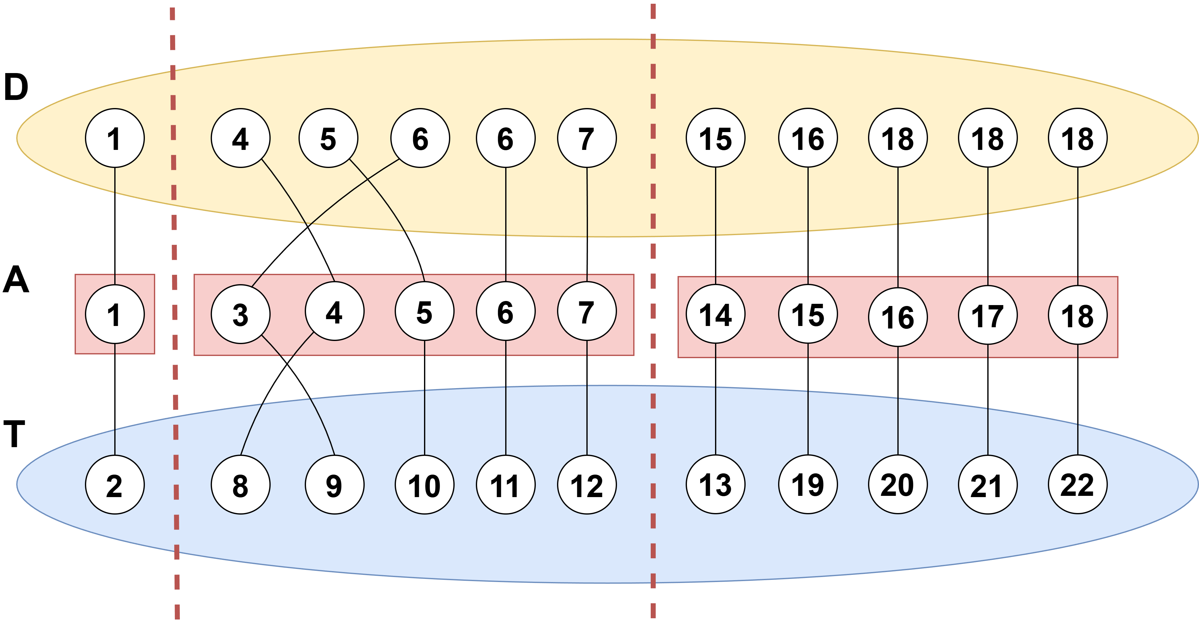
The next observation follows from Def. 8 and is one of the reasons for the usefulness of clusters.

Observation 16.

Let $A=\langle a_{1},\ldots,a_{n}\rangle$ be the discretized sequence of $D=\{d_{1},\ldots,d_{n}\}$ and let $C=\langle a_{i},\ldots,a_{j}\rangle$ be some cluster of $A$ . Then, $C$ is the discretized sequence of $\{d_{i},\ldots,d_{j}\}$ .

Lemma 17 (Self-reduction).

Position Matching reduces in time $\mathcal{O}(n)$ to solving a Position Matching instance for the numbers corresponding to each cluster.

Lemma 17 is heavily implied in [29], but not directly proven in the form that we desire for this work. For a formal proof we refer the reader to the full version of this paper [27]. See Figure 3 for some intuition for the proof.

2.2.3 Pinwheel variants and the concept of density

A quantity often used in Pinwheel Scheduling and its variants (see e.g., [2, 23, 30, 31, 36]) is the density of the input, defined as follows.

Definition 18 (Density).

For a (multi)set $D=\{d_{1},\ldots,d_{n}\}$ , its density is defined as $\mathrm{Dens}(D)=\sum_{i=1}^{n}1/d_{i}$ .

It is straightforward to prove that every Pinwheel Scheduling instance $D$ with $\mathrm{Dens}(D)>1$ admits no schedule (see [23] for a formal proof). On the other hand, it was recently proven that all Pinwheel Scheduling instances $D$ with $\mathrm{Dens}(D)\leq 5/6$ admit a schedule [30]. Note that this density threshold is tight, due to the instance $I=\{2,3,1/\varepsilon\}$ with $\mathrm{Dens}(I)=5/6+\varepsilon$ , which admits no infinite schedule for every $\varepsilon>0$ [7, 18].

The aforementioned result by [30] implies that all $k$ -Visits instances $D$ with $\mathrm{Dens}(D)\leq 5/6$ admit a schedule, for all $k\geq 1$ : it suffices to take an infinite schedule and remove all visits except the $k$ first visits of each task, preserving feasibility (cf. [29]).

2.2.4 Exact Matching and variations

We give the definitions of Exact Matching and its weighted generalization, which we will use in Section 4. Exact Matching was introduced by Papadimitriou and Yannakakis [39] in 1982, where they conjectured that it is NP-complete. However, Mulmuley, Vazirani and Vazirani [37] showed that the problem admits a randomized polynomial-time algorithm, placing it in the complexity class $\mathrm{RP}$ . To this day, Exact Matching remains notorious for being one of the few natural problems that are in $\mathrm{RP}$ , but not known to be in $\mathrm{P}$ .

Definition 19 (Exact Matching).

Given a graph $G=(V,E)$ , a subset $E^{\prime}\subseteq E$ of red edges and a positive integer $k$ , the Exact Matching problem asks whether there exists a perfect matching in $G$ involving exactly $k$ red edges.

Definition 20 (EWPM).

Given a weighted graph $G=(V,E,w)$ and an integer $W$ , the Exact Weighted Perfect Matching $(\textnormal{{EWPM}})$ problem asks whether there exists a perfect matching $M$ in $G$ with $\sum_{e\in M}w(e)=W$ .

Theorem 21 (Gurjar et al. 2016 [19], El Maalouly 2023 [12]).

There is a polynomial-time reduction from EWPM with polynomially-bounded weights to Exact Matching. If the initial graph is bipartite, the resulting graph is also bipartite. If the initial EWPM instance has $n$ vertices, $m$ edges and weights bounded by $W$ , then the resulting Exact Matching instance has $\mathcal{O}(n+mW)$ vertices and $\mathcal{O}(mW)$ edges. The reduction runs in time $\mathcal{O}(mW)$ .

Note that EWPM is known to be NP-complete when its weights are exponential [19]. However, when its weights are polynomially bounded, it is in $\mathrm{RP}$ by Theorem 21.

3 Hardness of 2-Visits relative to maximum multiplicity

In this section we prove that 2-Visits remains strongly NP-complete even when the maximum multiplicity is $2$ , resolving an open question from [29]. Our chain of reductions starts from Numerical Matching with Target Sums (NMTS). See Figure 1 for an overview.

The key idea for our result in this section is that padding an input sequence with two copies of certain larger numbers forces the discretized sequence of the input to consist of consecutive numbers starting from $1$ , as demonstrated in the following example.

Example 22.

Consider input $\langle 2,4,5,8,8,10\rangle$ . Its discretized sequence is $\langle 2,4,5,7,8,10\rangle$ . Let us pad the input with $2$ copies of some larger numbers:

\langle 2,4,5,8,8,10,11,11,12,12,13,13,14,14\rangle.

Observe that the discretized sequence of the modified input is

\langle 1,2,3,4,5,6,7,8,9,10,11,12,13,14\rangle=[14].

Additionally, the maximum multiplicity of the modified input is $2$ (granted that the maximum multiplicity of the initial input was not already larger than $2$ ).

This greatly simplifies the Position Matching problem (and thus also 2-Visits): the second set used for the matching now becomes static and equal to $[n]$ , rendering reductions from classical numerical matching problems possible, while only increasing the maximum multiplicity of the input by at most $1$ . Before we utilize this idea in Section 3.3, we prove an NP-hardness result for an appropriate variant of NMTS, serving as the first building block in our reduction chain.

3.1 Restricting Numerical Matching with Target Sums

We build upon the work of Hulett et al. [25] (Theorem 6) in order to prove that NMTS remains hard even when one set is equal to $[n]$ and each of the other two sets consists of distinct numbers. To this end, we define the following restricted version of the problem, which we will use in our chain of reductions leading to 2-Visits.

Definition 23 (SRNMTS).

Given two (simple) sets of positive integers $A=\{a_{1},\ldots,a_{n}\}$ and $T=\{t_{1},\ldots,t_{n}\}$ , the Semi-restricted Numerical Matching with Target Sums $(\textnormal{{SRNMTS}})$ problem asks whether there is a subset $M$ of $A\times[n]\times T$ s.t. every $a_{i}\in A$ , $b\in[n]$ , $t_{i}\in T$ occurs exactly once in $M$ and for every triplet $(a,b,t)\in M$ it holds that $a+b=t$ .

We call this problem semi-restricted in order to distinguish from the Restricted Numerical 3-Dimensional Matching (RN3DM) problem defined by Yu et al. [41], in which two out of three sets are fixed (instead of just one). We remark that RN3DM is not known to be NP-hard for distinct inputs; on the contrary, the reduction from 3-Partition by Yu et al. [41] appears to rely heavily on padding the input with $\mathrm{poly}(n)$ duplicates of $0$ and some large number. Modifying this method to forgo duplicates does not seem straightforward, which is the reason why we do not use RN3DM for our reductions in this paper.

Observation 24.

For every non-trivial instance of NMTS, it holds that $\max(T)>\max(A)$ and $\max(T)>\max(B)$ ; otherwise, we have a trivial no-instance. Hence, we may assume that these inequalities hold for the following reduction from NMTS.

Theorem 25.

( $\star$ ) SRNMTS is strongly NP-complete.

3.2 From SRNMTS to IN3DM

We now use SRNMTS to obtain a stronger version of the IN3DM hardness theorem of [29].

Theorem 26.

( $\star$ ) IN3DM is strongly NP-complete even when $A$ and $T$ are simple sets.

3.3 From IN3DM to Position Matching

In this subsection we present a reduction from IN3DM to Position Matching that increases the maximum multiplicity of the first set by at most $1$ , while preserving the maximum multiplicity of the target set $T$ . Note that $T$ containing only distinct integers is crucial for the reduction from Position Matching to 2-Visits (cf. [29]). Additionally, recall that Position Matching can be solved in polynomial time when the input consists solely of simple sets (Lemma 13), while IN3DM is strongly NP-complete even in that case (Theorem 26). Thus, concerning multiplicity preservation, this is the best possible reduction unless $\mathrm{P}=\mathrm{NP}$ .

We first present an auxiliary lemma that bounds the values of elements in IN3DM.

Lemma 27.

( $\star$ ) IN3DM is NP-complete, even when all the following properties hold.

1.

$\min(A)\geq n$ .
2.

There is some polynomial $P(n)$ such that $\max(A)\leq P(n)$ and $\max(T)\leq P(n)$ .
3.

$A$ and $T$ are simple sets.

Recall that for Position Matching the second set is the discretized sequence (Def. 8) of the first one and for any triplet $(a,b,t)$ in its solution it must hold that $a\geq b$ and $a+b\geq t$ . Most of the technical difficulty of the following reduction stems from these restrictions. The main idea is to pad the first set with duplicate numbers in order to force its discretized sequence to consist of consecutive numbers starting from $1$ (like the second set of IN3DM). See Example 22 for some intuition regarding this transformation. At the same time, we utilize the $\min(A)\geq n$ inequality from Lemma 27 to force all candidate triplets $(a,b,t)$ to satisfy $a\geq b$ , thus rendering that restriction irrelevant and forcing an equivalence between IN3DM and Position Matching.

We are now ready to present our reduction to Position Matching.

Theorem 28 (Main reduction).

( $\star$ ) There is a polynomial-time reduction from IN3DM to Position Matching, such that all elements added to the input have multiplicity at most $2$ and values polynomial in $n$ .

We obtain the following corollary from Theorem 28 and Lemma 27.

Corollary 29.

Position Matching is strongly NP-complete even when the maximum multiplicity of $D$ is equal to $2$ .

3.4 From Position Matching to 2-Visits

Observation 30.

The reduction from Position Matching to 2-Visits by Kanellopoulos et al. [29] preserves the maximum multiplicity. More specifically, for a Position Matching instance $(D,T)$ it requires $T$ to be a simple set and it constructs the set of deadlines for 2-Visits by padding $D$ with distinct numbers that are either smaller than $\min(D)$ or larger than $\max(D)$ .

We obtain the main result of this section by combining Corollary 29 with Observation 30.

Theorem 31.

2-Visits is strongly NP-complete even when the maximum multiplicity of the input is equal to $2$ .

We thus obtain the following corollary, settling an open question stated by [29] in SODA 2026 and contrasting the tractability of 2-Visits for simple sets (Lemma 13).

Corollary 32.

There is no FPT or XP algorithm for 2-Visits parameterized by the maximum multiplicity, unless $\mathrm{P}=\mathrm{NP}$ .

4 2-Visits parameterized by the number of distinct numbers

In this section we prove that Position Matching is in $\mathrm{RP}$ when the number of distinct numbers in $D$ (or simply number of numbers) is constant, by reducing it to Exact Weighted Perfect Matching (EWPM–Def. 20). This naturally transfers to 2-Visits through Corollary 11.

Let $p$ be the number of numbers of the input set $D$ of Position Matching. The main idea of the following reduction is to model Position Matching as a bipartite matching instance between $A$ and $T$ , while modeling $D$ as edge weights. Bounding $p$ allows these weights to be polynomial, which is important for EWPM (see Section 2.2.4). We remark that it only makes sense to bound the number of numbers of $D$ , since $A$ and $T$ both consist of distinct numbers by definition.

Theorem 33.

( $\star$ ) There is a reduction from Position Matching to EWPM in multigraphs with $\mathcal{O}(n^{2}p)$ edges and weights bounded by $\mathcal{O}(n^{p-1})$ , running in time $\mathcal{O}(n^{2}p)$ .

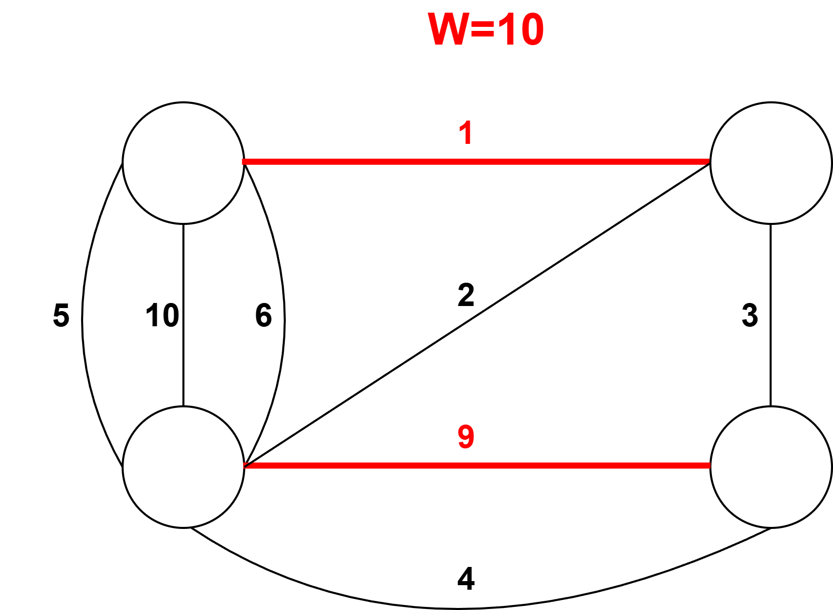
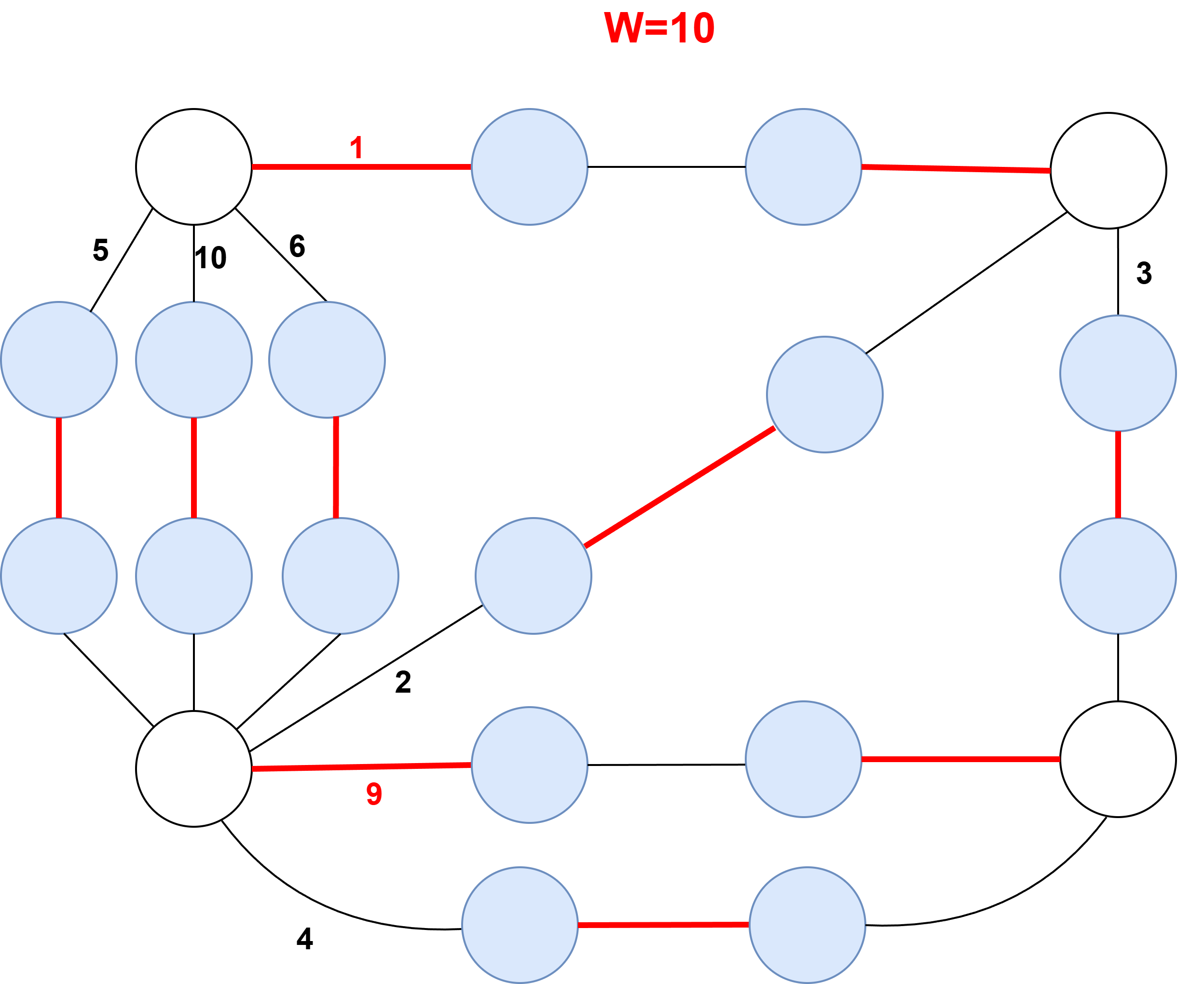
To the best of our knowledge, Exact Matching and EWPM have not been considered in multigraphs, although it is likely that some of their results generalize to multigraphs easily. We thus include Lemma 34 for the sake of completeness. Its proof is a standard transformation of a multigraph to a simple graph by replacing edges with paths (see Figure 4). Note that for the purposes of this work we only need the following reduction for bipartite multigraphs, although it holds even for general multigraphs.

Lemma 34.

( $\star$ ) There is a linear-time reduction from EWPM in multigraphs to EWPM in simple graphs, preserving weights and multiplying the amount of edges by $3$ .

We obtain the following through Theorems 21, 33 and Lemma 34.

Theorem 35.

Position Matching reduces in $\mathcal{O}(n^{p+1}p)$ time to Exact Matching with $\mathcal{O}(n^{p+1}p)$ vertices and edges.

Combining this with Corollary 11 and Lemma 17, we obtain the main result of this section.

Theorem 36.

2-Visits reduces in $\mathcal{O}(n^{p+1}p)$ time to solving an Exact Matching instance with $\mathcal{O}(n^{p+1}p)$ vertices and edges for each cluster of the input’s discretized sequence, where $p$ is the maximum number of distinct deadlines corresponding to a cluster.

We obtain the following corollary through the well-known result by Mulmuley et al. [37] for Exact Matching (see Section 2.2.4).

Corollary 37.

2-Visits is in $\mathrm{RP}$ when there is a constant amount of distinct deadlines corresponding to each cluster of the input’s discretized sequence.

We thus make progress towards the open question in [29] about the parameterization of 2-Visits by the number of numbers. Although we showed that 2-Visits admits the equivalent of a randomized XP algorithm parameterized by the number of numbers, it still remains open whether it admits a deterministic XP or FPT algorithm with the same parameter.

Note that we do not actually use the number of distinct deadlines of the whole input as parameter; due to Lemma 17, it suffices to use the number of distinct deadlines corresponding to the same cluster.

Observation 38.

The graphs obtained from Theorems 35 and 36 are bipartite, since the multigraph of Theorem 33 is bipartite, while Lemma 34 and Theorem 21 both preserve this graph property (due to only replacing edges with paths of odd length). Thus, any algorithm for Exact Matching in bipartite graphs is applicable to 2-Visits through Theorem 36.

Although we do not use Observation 38 in this work, since the algorithm of Mulmuley et al. [37] works for general graphs, we include it as it may be useful in future research.

5 Density thresholds of $k$ -Visits

In this section we study the density thresholds of the $k$ -Visits problem, for various values of $k$ . See Section 2.2.3 for a summary on the concept of density. We use the following terminology:

$\blacksquare$

We refer to the maximum value of density up to which all instances of a problem admit a schedule as the lower density threshold of the respective problem.
$\blacksquare$

We refer to the minimum value of density above which no instance of a problem admits a schedule as the upper density threshold of the respective problem.

Recall that for the infinite version of the problem (i.e., Pinwheel Scheduling) the lower density threshold is $5/6$ [30] and the upper density threshold is $1$ [23]. Both of these thresholds are tight.

5.1 A tight lower density threshold for 1-Visit

Lemma 39.

Every 1-Visit instance $D=\{d_{1},\ldots,d_{n}\}$ with $\mathrm{Dens}(D)\leq 1$ admits a schedule.

Proof.

We assume $d_{1}\leq\ldots\leq d_{n}$ , as is standard. Every 1-Visit instance with no feasible schedule must contain a deadline $d_{j},\ j\in[n]$ , such that $d_{j}<j$ ; otherwise, the schedule $1,\ldots,n$ would be feasible. We now seek to minimize the density of such an instance. Since both adding more deadlines to $D$ and decreasing the value of a deadline only increases $\mathrm{Dens}(D)$ , we set $d_{j}$ to be the largest element of $D$ , with value $d_{j}=j-1$ . Additionally, the largest value that each $d_{i},\ i\in[j-1]$ , can take without violating the non-decreasing order of the deadlines is equal to $j-1$ , i.e., the value of $d_{j}$ . Hence, the density of a 1-Visit instance that does not admit a schedule cannot be smaller than

\sum_{i=1}^{j}\frac{1}{d_{i}}=\sum_{i=1}^{j}\frac{1}{j-1}=\frac{j}{j-1}>1,\;% \forall j\in\mathbb{N}.

We infer that every 1-Visit instance $D$ with $\mathrm{Dens}(D)\leq 1$ admits a feasible schedule. $\hfill\blacktriangleleft$

Lemma 40.

For all $\varepsilon>0$ , there exists a 1-Visit instance $D$ with $1<\mathrm{Dens}(D)<1+\varepsilon$ that admits no schedule.

Proof.

The instance $D=\{n-1,\ldots,n-1\}$ (with $n=|D|$ ) trivially admits no 1-Visit schedule, since $\max(D)<n$ . Its density is $\mathrm{Dens}(D)=n/(n-1)$ , which is arbitrarily close to $1$ for large values of $n$ . $\hfill\blacktriangleleft$

We obtain the following theorem from Lemmas 39, 40.

Theorem 41.

1-Visit has a tight lower density threshold of $1$ .

5.2 Bounds for the lower density threshold of 2-Visits

The following lemma is the key to our density bound for 2-Visits and we regard it as our main technical contribution in this section. We begin by taking it for granted and defer its proof to Section 5.2.1.

Lemma 42 (Main Lemma).

Let $D=\{d_{1},\ldots,d_{n}\}$ be a 2-Visits instance with discretized sequence $A=\langle a_{1},\ldots,a_{n}\rangle$ , and define $T=[2n]\setminus A=\{t_{1},\ldots,t_{n}\}$ . If $\mathrm{Dens}(D)\leq\sqrt{2}-1/2$ , then it holds that $|T\cap[d_{i}+a_{i}]|\geq i$ , for all $i\in[n]$ .

Note that, as usual, we assume that the elements in $D$ , $A$ and $T$ are sorted in non-decreasing order. Additionally, by Remark 4 we have $a_{n}\leq d_{n}\leq 2n$ , which implies $|T|=n$ .

Lemma 43.

Every 2-Visits instance $D=\{d_{1},\ldots,d_{n}\}$ with $\mathrm{Dens}(D)\leq\sqrt{2}-1/2$ admits a schedule. The respective schedule can be constructed in time $\mathcal{O}(n)$ .

Proof.

Let $D=\{d_{1},\ldots,d_{n}\}$ , $d_{1}\leq d_{2}\leq\cdots\leq d_{n}$ , be a 2-Visits instance with $\mathrm{Dens}(D)\leq\sqrt{2}-1/2$ and let $A=\langle a_{1},\ldots,a_{n}\rangle$ be the discretized sequence of $D$ . Define $T=[2n]\setminus A=\{t_{1},\ldots,t_{n}\}$ . By Lemma 42, we have $|T\cap[d_{i}+a_{i}]|\geq i$ , for all $i\in[n]$ . This is directly equivalent to

t_{i}\leq d_{i}+a_{i},\text{ for all }i\in[n].

(1)

We construct a feasible 2-Visits schedule as follows. For each task $i\in[n]$ , we place the primary visit of task $i$ in position $a_{i}$ and the secondary visit of task $i$ in position $t_{i}$ . By Definition 8, it holds that $d_{i}\geq a_{i},\ \forall i\in[n]$ , hence the suggested placement of primary visits is feasible. By Equation (1), the suggested placement of secondary visits is also feasible, given the aforementioned placement of primary visits. $\hfill\blacktriangleleft$

Theorem 44.

The lower density threshold of 2-Visits is at least $\sqrt{2}-1/2\approx 0.9142$ and at most $1$ .

Proof.

The former part follows from Lemma 43. Since every instance that admits a 2-Visits schedule also (trivially) admits a 1-Visit schedule, the lower density threshold of 2-Visits cannot be larger than $1$ , due to Theorem 41. $\hfill\blacktriangleleft$

5.2.1 Proof of Lemma 42

We will now prove Lemma 42. We split the proof into multiple auxiliary lemmas, as it is quite technical. Consider the following property, which is the negation of the property mentioned in Lemma 42.

\exists i\in[n]:|T\cap[d_{i}+a_{i}]|\leq i-1.

(2)

Let $D^{\star}=\{d_{1}^{\star},\ldots d_{n}^{\star}\}$ be an instance satisfying (2) with the minimum possible density. Proving $\mathrm{Dens}(D^{\star})>\sqrt{2}-1/2$ directly implies Lemma 42. We will construct $D^{\star}$ and compute its density.

Let $A^{\star}=\langle a_{1}^{\star},\ldots,a_{n}^{\star}\rangle$ be the discretized sequence of $D^{\star}$ and $T^{\star}=[2n]\setminus A^{\star}$ . Let $j\in[n]$ be the smallest index for which $|T^{\star}\cap[d_{j}^{\star}+a_{j}^{\star}]|\leq j-1$ . We sequentially restrict the form of $D^{\star}$ as follows.

Lemma 45.

( $\star$ ) $|T^{\star}\cap[d_{j}^{\star}+a_{j}^{\star}]|=j-1$ .

Lemma 46.

( $\star$ ) The $j-1$ numbers in $|T^{\star}\cap[d_{j}^{\star}+a_{j}^{\star}]|$ are the smallest possible, i.e. $T^{\star}\cap[d_{j}^{\star}+a_{j}^{\star}]=[j-1]$ . Consequently, $j,\ldots,d_{j}^{\star}+a_{j}^{\star}\in A^{\star}$ .

Lemma 47.

( $\star$ ) $a_{j}^{\star}=2j-1$ and $d_{n}^{\star}\geq d_{j}^{\star}+2j-1$ .

Lemma 48.

( $\star$ ) $A^{\star}=\langle j,\ldots,d_{n}^{\star}\rangle$ .

Lemma 48 implies $n=d_{n}^{\star}-j+1$ . For $D^{\star}$ to be density-minimizing, it must hold that:

$\blacksquare$

The first $j$ deadlines are equal to $d_{j}^{\star}$ .
$\blacksquare$

The other $d_{n}^{\star}-2j+1$ deadlines are equal to $d_{n}^{\star}$ .

If either of the above does not hold, replacing the deadlines that do not follow these rules with the ones suggested by them can only decrease the density, leading to a contradiction.

Observe that the density of the $d_{n}^{\star}-2j+1$ largest deadlines is $\frac{d_{n}^{\star}-2j+1}{d_{n}^{\star}}$ , which is increasing with respect to $d_{n}^{\star}$ . Combining this with Lemma 47, we obtain $d_{n}^{\star}=d_{j}^{\star}+2j-1$ and thus $n=j+d_{j}^{\star}$ . Hence, $D^{\star}$ is the two-level multiset

D^{\star}=\Bigl\{\ \underbrace{d_{j}^{\star},\ldots,d_{j}^{\star}}_{j\ \text{% copies}}\ ,\ \underbrace{d_{j}^{\star}+2j-1,\ldots,d_{j}^{\star}+2j-1}_{d_{j}^% {\star}\ \text{copies}}\ \Bigr\},\qquad d_{j}^{\star}\geq a_{j}^{\star}=2j-1.

The density of $D^{\star}$ is

\mathrm{Dens}(D^{\star})=\frac{j}{d_{j}^{\star}}+\frac{d_{j}^{\star}}{d_{j}^{% \star}+2j-1}.

This function is minimized when $j=\left[\left(\sqrt{2}-1\right)/2\right]\cdot d_{j}^{\star}+1/2$ and $d_{j}^{\star}\to\infty$ , in which case its infimum equals $\sqrt{2}-1/2$ (see the full version of this paper [27] for a proof and Figure 5 for a plot of the function). Thus, we obtain $\mathrm{Dens}(D^{\star})>\sqrt{2}-1/2$ , which proves Lemma 42.

5.3 Bounds for the lower density threshold of $k$ -Visits

In the following we prove a lemma that connects $k$ -Visits to Pinwheel Scheduling and use it to obtain an upper bound for the lower density threshold of the former.

Lemma 49 is a straightforward modification of the PSPACE-membership proof for Pinwheel Scheduling by Holte et al. [23]. We denote the sub-schedule of a schedule $S$ consisting of the positions from $p$ up to $q\geq p$ as $S[p,\,q]$ .

Lemma 49 (Cyclic schedule).

( $\star$ ) Let $S$ be a feasible schedule for a $k$ -Visits instance $D=\{d_{1},\ldots,d_{n}\}$ and let $m=\prod_{i}d_{i}$ . If for all $i\in[n]$ the $k$ -th visit of task $i$ occurs no earlier than position $m+1$ , then there exist positions $p,\,p^{\prime}\in[m]$ , $p\leq p^{\prime}$ , such that $S[p,\,p^{\prime}]$ can induce a feasible schedule for the respective Pinwheel Scheduling instance by infinitely repeating itself.

Theorem 50.

The lower density threshold of $k$ -Visits is at most $5/6+1/\lfloor(k-1)/6\rfloor$ , for all $k\in\mathbb{N}$ .

Proof.

Consider the instance $D(x)=\{d_{1}=2,\,d_{2}=3,\,d_{3}=x\}$ , $x\in\mathbb{N}$ , and observe that it is a no-instance of Pinwheel Scheduling for all $x\in\mathbb{N}$ : each of the first two tasks has to be visited once every two time units in an infinite schedule, hence any schedule fails at the $x$ -th time unit (cf. [7]).

Set $k=\prod_{i}d_{i}+1=6x+1$ and assume $D(x)$ admits a $k$ -Visits schedule. Clearly, the $k$ -th visit of any task cannot occur earlier than position $k$ , thus the conditions of Lemma 49 are satisfied for this $k$ . We obtain that $D(x)$ is a yes-instance of Pinwheel Scheduling, which is a contradiction. We infer that for all $x\in\mathbb{N}$ , $D(x)$ is a no-instance of $k$ -Visits with $k=6x+1$ . Since $\mathrm{Dens}(D(x))=5/6+1/x$ , this proves the desired statement when $k\equiv 1\pmod{6}$ .

For $k\not\equiv 1\pmod{6}$ , it suffices to observe that if an instance admits no $k$ -Visits schedule, then it does not admit a $k^{\prime}$ -Visits schedule for any $k^{\prime}>k$ (cf. [29]). $\hfill\blacktriangleleft$

We obtain the following corollary by combining Theorem 50 with the fact that the lower density threshold of $k$ -Visits cannot be smaller than $5/6$ (see Section 2.2.3 for a short explanation).

Corollary 51.

The lower density threshold of $k$ -Visits approaches $5/6$ for $k\rightarrow\infty$ , which is known to be tight for Pinwheel Scheduling [30].

5.4 Nonexistence of upper density threshold for $k$ -Visits

Theorem 52.

For all $k\in\mathbb{N}$ and all $\delta>0$ , there exists an instance $D$ with $\mathrm{Dens}(D)>\delta$ that admits a $k$ -Visits schedule. Equivalently, there is no upper density threshold for $k$ -Visits, for any $k\in\mathbb{N}$ .

Proof.

Fix $k\in\mathbb{N}$ and consider the instance $D(n)=\{1,\ 1+k,\ 1+2k,\ldots,1+(n-1)k\}$ . It is clear that $D(n)$ admits a $k$ -Visits schedule for all $n\in\mathbb{N}$ : it suffices to visit the first task $k$ times consecutively, then the second task $k$ times consecutively, and so on. Note that

\mathrm{Dens}(D(n))=\sum_{i=0}^{n-1}\frac{1}{1+ik}

is a harmonic series for $n\rightarrow\infty$ , which is a well-known divergent series. Hence, for large values of $n$ , $\mathrm{Dens}(D(n))$ is arbitrarily large, which immediately implies the theorem. $\hfill\blacktriangleleft$

6 The (1 or 2)-Visits problem

In this section we define and study the (1 or 2)-Visits problem, a generalization of 2-Visits.

Definition 53 ((1 or 2)-Visits).

Given positive integers $m, n$ and a (multi)set of positive integers (deadlines) $D=\{d_{1},\ldots,d_{m+n}\}$ , the (1 or 2)-Visits problem asks whether there exists a schedule of length $m+2n$ visiting exactly one task $i\in[m+n]$ per time unit, such that:

$\blacksquare$

For each $i\in[m]$ , task $i$ is visited exactly once within the first $d_{i}$ positions of the schedule.
$\blacksquare$

For each $i\in[m+1,m+n]$ , task $i$ is visited twice: once within the first $d_{i}$ positions of the schedule, and once at most $d_{i}$ positions after its first visit.

As usual, we assume $d_{1}\leq\ldots\leq d_{m}$ and $d_{m+1}\leq\ldots\leq d_{m+n}$ . For tasks $i\in[m+1,m+n]$ , we can (equivalently) say that a primary visit of $i$ occurs within the first $d_{i}$ positions of the schedule and a secondary visit of $i$ occurs at most $d_{i}$ positions after its primary visit or at any position before its primary visit, as is standard for 2-Visits. This alternative definition will allow us to prove a property that disconnects the positions in which primary visits are placed from those in which secondary visits are placed, similar to [29]. For the tasks that only require one visit, we use the term single visits.

It is immediate that (1 or 2)-Visits is strongly NP-complete, as 2-Visits constitutes its special case with $m=0$ . Hence, the focus of this section is to generalize the existing positive results for 2-Visits to (1 or 2)-Visits. To this end, we reduce (1 or 2)-Visits to Position Matching.

6.1 Reduction to Position Matching

Let $D=\{d_{1},\ldots,d_{m+n}\}$ be a (1 or 2)-Visits input with $m$ tasks that have to be visited once and $n$ tasks that have to be visited twice. For the latter, we will use primary and secondary visits, as explained above. We assume that $d_{i}\leq m+2n$ for all $i\in[m+n]$ . Note that if there was a deadline larger than $m+2n$ in the input, then all visits of the respective task could be placed at the end of the schedule without affecting its feasibility and, thus, the respective deadline could be removed from the input to obtain an equivalent (1 or 2)-Visits instance.

Let $A=\langle a_{1},\ldots,a_{n}\rangle$ be the discretized sequence of $\langle d_{m+1},\ldots,d_{m+n}\rangle$ . We will prove that it suffices to place the primary visits of tasks $m+1,\ldots,m+n$ in a permutation of the positions in $A$ (analogous to Lemma 10).

Lemma 54.

( $\star$ ) A (1 or 2)-Visits instance $D=\{d_{1},\ldots,d_{m+n}\}$ admits a schedule if and only if it admits a schedule in which all $n$ primary visits are placed in a permutation of the positions of the discretized sequence $A=\langle a_{1},\ldots,a_{n}\rangle$ of $\langle d_{m+1},\ldots,d_{m+n}\rangle$ .

With Lemma 54, we have disconnected the positions in which primary visits should be placed from the positions in which single and secondary visits should be placed. We now disconnect the latter two as well.

Lemma 55 (Disconnection).

( $\star$ ) A (1 or 2)-Visits instance $D\!=\!\{d_{1},\ldots,d_{m+n}\}$ , with $A=\langle a_{1},\ldots,a_{n}\rangle$ being the discretized sequence of $\langle d_{m+1},\ldots,d_{m+n}\rangle$ , admits a schedule if and only if it admits a schedule such that

1.

The $n$ primary visits are placed in some permutation of the positions in $A$ .
2.

The $m$ single visits are placed in order of non-decreasing deadline in the latest feasible positions of $[m+2n]\setminus A$ .
3.

The $n$ secondary visits are placed in some permutation of the $n$ remaining positions.

We are now ready to reduce (1 or 2)-Visits to Position Matching.

Theorem 56.

( $\star$ ) (1 or 2)-Visits reduces to Position Matching in time $\mathcal{O}(n+m)$ .

6.2 Algorithms for (1 or 2)-Visits

We are now ready to generalize all known algorithms for 2-Visits to (1 or 2)-Visits. Let $A=\langle a_{1},\ldots,a_{n}\rangle$ be the discretized sequence of $\langle d_{m+1},\ldots,d_{m+n}\rangle$ .

Theorem 57.

( $\star$ ) (1 or 2)-Visits admits the following algorithms:

1.

An algorithm running in $\mathcal{O}(m+n!)$ time.⁶⁶6Note that the naive brute force algorithm for (1 or 2)-Visits runs in time $\mathcal{O}((m+2n)!)$ .
2.

An algorithm running in $\mathcal{O}(m+n)$ time, if $d_{m+1},\ldots,d_{m+n}$ are distinct numbers.
3.

An algorithm running in $\mathcal{O}(m+n)$ time, if there are at most two distinct deadlines corresponding to each cluster of $A$ .
4.

An FPT algorithm parameterized by the maximum cluster size $c$ of $A$ , running in $\mathcal{O}(m+n\cdot c!)$ time.
5.

A randomized polynomial-time $\mathrm{(RP)}$ algorithm, if there is a constant number of distinct deadlines corresponding to each cluster of $A$ .

$\blacktriangleright$ Remark 58.

The algorithms of Theorem 57 coincide with the state-of-the-art algorithms for 2-Visits when $m=0$ .

7 3-Visits violates the key structural properties of 2-Visits

In this section we provide a counterexample that shows that Lemma 10 and the algorithm implied by Lemma 13 do not hold for 3-Visits. This is significant for future work, since the vast majority of results for 2-Visits (both positive and negative) heavily rely on these lemmas; it seems that new methods are yet to be discovered in order to efficiently study $k$ -Visits for $k>2$ .

Lemma 59.

( $\star$ ) There is a yes-instance of 3-Visits for which every feasible schedule contains at least two visits of the same task in the positions of the discretized sequence, violating Lemma 10.

$\blacktriangleright$ Remark 60.

The violation of Lemma 10 is significant because all existing positive results for 2-Visits and its generalization, (1 or 2)-Visits (see Theorem 57 for a list of these results), currently rely on Lemma 10 (and its generalization, Lemma 54). In fact, even the NP-hardness of 2-Visits strongly relies on Lemma 10.

Lemma 61.

( $\star$ ) There is a yes-instance of 3-Visits with distinct numbers for which every feasible schedule places the first visits in non-sorted order, violating a property of the algorithm implied by Lemma 13.

It is straightforward to see that the algorithm implied by Lemma 13 (for 2-Visits with distinct deadlines) places primary visits in sorted order in the positions of the discretized sequence and secondary visits in sorted order in the rest of the positions. This implies that first visits are placed in sorted order (by non-decreasing deadline), with the same also holding for second visits. With Lemma 61 we prove that this property is violated for 3-Visits, reinforcing the following conjecture from [29].

Conjecture 62.

3-Visits is strongly NP-complete even when the input is a simple set.

8 Conclusion

Our work highlights several interesting properties of 2-Visits. Although this problem was conceived as a finite version of Pinwheel Scheduling, mainly as a stepping stone for studying its complexity, it turns out to be quite interesting in its own right. As highlighted in [29], 2-Visits is one of the rare natural problems that is in $\mathrm{P}$ for simple sets, but $\mathrm{NP}$ -complete when multisets are allowed. We further enhance this contrast by unexpectedly answering a question of that paper in the negative, proving that 2-Visits is in fact strongly $\mathrm{NP}$ -complete even with at most two copies of each number. We find this result both intriguing and surprising, as it contradicts our intuition.

A natural question arising now is whether 2-Visits can be parameterized by the number of duplicates, which is possible despite its $\mathrm{NP}$ -completeness for maximum multiplicity $2$ . Another question remaining open regards the parameterization of 2-Visits by the number of numbers. We conjecture that Position Matching (and thus also 2-Visits) is FPT by the number of numbers of $D$ , as is standard for numerical matching variants [14]. However, as explained in Section 1.1, the standard method of showing this by reduction to Integer Linear Programming [14] fails for Position Matching. Our result in Section 4 indicates that 2-Visits is likely tractable when parameterized by the number of numbers, although the existence of a deterministic XP or FPT algorithm remains open.

Another open question is whether our bound for the lower density threshold of 2-Visits in Section 5 is tight, as well as whether the $\sqrt{2}-1/2$ number that we obtained can provide insight into generalizing our result to $k$ -Visits with $k>2$ . We believe that studying the lower density threshold of $k$ -Visits in relation to $k$ is a particularly interesting direction for future work, as it would complement the known $(5/6)$ -threshold of Pinwheel Scheduling [30]. Perhaps computer-assisted brute force (like the ones used in [18, 30, 36] for infinite versions) can also prove useful for the density thresholds of finite versions. Since we could not find any unschedulable 2-Visits instance with density smaller than or equal to $1$ , it is possible that the lower density threshold of 2-Visits is exactly $1$ . However, this would imply that 1-Visit and 2-Visits share the same threshold, which seems counterintuitive in conjunction with Corollary 51.

Arguably the most interesting and seemingly difficult direction for future work would be to generalize results of 2-Visits to $k>2$ . Currently, none of the algorithms for 2-Visits seem to transfer to 3-Visits and, in fact, even proving the NP-hardness of 3-Visits seems exceptionally challenging, despite strong intuition in favor of it. Our example in Section 7 highlights the reasons why results from 2-Visits do not currently transfer to 3-Visits and reinforces the conjecture by [29] that 3-Visits is strongly NP-complete even for simple sets. Transferring (strong) NP-hardness to $k$ -Visits for larger $k$ would be particularly useful if one could also transfer it to Pinwheel Scheduling, which would settle a question open since 1989. This may actually be possible, since the existence of an infinite schedule is known to be equivalent to the existence of an infinite schedule with finite period [23]. Our Lemma 49 establishes another similar connection between finite and infinite versions, further highlighting the relationship between the two problems.

One last open question we would like to highlight is whether RN3DM (defined by Yu et al. [41]) remains strongly NP-complete for simple sets. If this holds, it would simplify the first two steps of our reduction chain in Section 3, as there would be no need to consider the more complicated NMTS problem. However, the existing hardness proof for RN3DM [41] heavily relies on padding 3-Partition with duplicate numbers. We believe that settling this question would require a reduction significantly different from the existing one.

References

[1] Annelieke C. Baller, Martijn van Ee, Maaike Hoogeboom, and Leen Stougie. Complexity of inventory routing problems when routing is easy. Networks, 75(2):113–123, 2020. doi:10.1002/NET.21908.
[2] Amotz Bar-Noy, Richard E. Ladner, and Tami Tamir. Windows scheduling as a restricted version of bin packing. ACM Trans. Algorithms, 3(3):28, 2007. doi:10.1145/1273340.1273344.
[3] Yuriy Biktairov, Leszek Gasieniec, Wanchote Po Jiamjitrak, Namrata, Benjamin Smith, and Sebastian Wild. Simple approximation algorithms for polyamorous scheduling. In Ioana Oriana Bercea and Rasmus Pagh, editors, 2025 Symposium on Simplicity in Algorithms, SOSA 2025, New Orleans, LA, USA, January 13-15, 2025, pages 290–314. SIAM, 2025. doi:10.1137/1.9781611978315.23.
[4] Lélia Blin, Alessia Milani, Maria Potop-Butucaru, and Sébastien Tixeuil. Exclusive perpetual ring exploration without chirality. In Distributed Computing, 24th International Symposium, DISC 2010, Cambridge, MA, USA, September 13-15, 2010. Proceedings, pages 312–327, 2010. doi:10.1007/978-3-642-15763-9_29.
[5] Thomas Bosman, Martijn van Ee, Yang Jiao, Alberto Marchetti-Spaccamela, R. Ravi, and Leen Stougie. Approximation algorithms for replenishment problems with fixed turnover times. Algorithmica, 84(9):2597–2621, 2022. doi:10.1007/S00453-022-00974-4.
[6] Mee Yee Chan and Francis Y. L. Chin. General schedulers for the pinwheel problem based on double-integer reduction. IEEE Trans. Computers, 41(6):755–768, 1992. doi:10.1109/12.144627.
[7] Mee Yee Chan and Francis Y. L. Chin. Schedulers for larger classes of pinwheel instances. Algorithmica, 9(5):425–462, 1993. doi:10.1007/BF01187034.
[8] Huda Chuangpishit, Jurek Czyzowicz, Leszek Gasieniec, Konstantinos Georgiou, Tomasz Jurdzinski, and Evangelos Kranakis. Patrolling a path connecting a set of points with unbalanced frequencies of visits. In SOFSEM 2018: Theory and Practice of Computer Science - 44th International Conference on Current Trends in Theory and Practice of Computer Science, Krems, Austria, January 29 - February 2, 2018, Proceedings, pages 367–380, 2018. doi:10.1007/978-3-319-73117-9_26.
[9] Jurek Czyzowicz, Kostantinos Georgiou, and Evangelos Kranakis. Patrolling. In Paola Flocchini, Giuseppe Prencipe, and Nicola Santoro, editors, Distributed Computing by Mobile Entities, Current Research in Moving and Computing, volume 11340 of Lecture Notes in Computer Science, pages 371–400. Springer, 2019. doi:10.1007/978-3-030-11072-7_15.
[10] Peter Damaschke. Two robots patrolling on a line: Integer version and approximability. In Combinatorial Algorithms - 31st International Workshop, IWOCA 2020, Bordeaux, France, June 8-10, 2020, Proceedings, pages 211–223, 2020. doi:10.1007/978-3-030-48966-3_16.
[11] Mattia D’Emidio, Gabriele Di Stefano, and Alfredo Navarra. Bamboo garden trimming problem: Priority schedulings. Algorithms, 12(4):74, 2019. doi:10.3390/A12040074.
[12] Nicolas El Maalouly. Exact Matching: Algorithms and Related Problems. In Petra Berenbrink, Patricia Bouyer, Anuj Dawar, and Mamadou Moustapha Kanté, editors, 40th International Symposium on Theoretical Aspects of Computer Science (STACS 2023), volume 254 of Leibniz International Proceedings in Informatics (LIPIcs), pages 29:1–29:17, Dagstuhl, Germany, 2023. Schloss Dagstuhl – Leibniz-Zentrum für Informatik. doi:10.4230/LIPIcs.STACS.2023.29.
[13] Nicolas El Maalouly, Sebastian Haslebacher, Adrian Taubner, and Lasse Wulf. On Finding l-Th Smallest Perfect Matchings. In Anne Benoit, Haim Kaplan, Sebastian Wild, and Grzegorz Herman, editors, 33rd Annual European Symposium on Algorithms (ESA 2025), volume 351 of Leibniz International Proceedings in Informatics (LIPIcs), pages 19:1–19:15, Dagstuhl, Germany, 2025. Schloss Dagstuhl – Leibniz-Zentrum für Informatik. doi:10.4230/LIPIcs.ESA.2025.19.
[14] Michael R. Fellows, Serge Gaspers, and Frances A. Rosamond. Parameterizing by the number of numbers. Theory Comput. Syst., 50(4):675–693, 2012. doi:10.1007/S00224-011-9367-Y.
[15] Peter C. Fishburn and J. C. Lagarias. Pinwheel scheduling: Achievable densities. Algorithmica, 34(1):14–38, 2002. doi:10.1007/S00453-002-0938-9.
[16] Leszek Gasieniec, Tomasz Jurdzinski, Ralf Klasing, Christos Levcopoulos, Andrzej Lingas, Jie Min, and Tomasz Radzik. Perpetual maintenance of machines with different urgency requirements. J. Comput. Syst. Sci., 139:103476, 2024. doi:10.1016/J.JCSS.2023.103476.
[17] Leszek Gasieniec, Ralf Klasing, Christos Levcopoulos, Andrzej Lingas, Jie Min, and Tomasz Radzik. Bamboo garden trimming problem (perpetual maintenance of machines with different attendance urgency factors). In SOFSEM 2017: Theory and Practice of Computer Science - 43rd International Conference on Current Trends in Theory and Practice of Computer Science, Limerick, Ireland, January 16-20, 2017, Proceedings, volume 10139 of Lecture Notes in Computer Science, pages 229–240. Springer, 2017. doi:10.1007/978-3-319-51963-0_18.
[18] Leszek Gasieniec, Benjamin Smith, and Sebastian Wild. Towards the 5/6-density conjecture of pinwheel scheduling. In Cynthia A. Phillips and Bettina Speckmann, editors, Proceedings of the Symposium on Algorithm Engineering and Experiments, ALENEX 2022, Alexandria, VA, USA, January 9-10, 2022, pages 91–103. SIAM, 2022. doi:10.1137/1.9781611977042.8.
[19] Rohit Gurjar, Arpita Korwar, Jochen Messner, Simon Straub, and Thomas Thierauf. Planarizing gadgets for perfect matching do not exist. ACM Trans. Comput. Theory, 8(4):14:1–14:15, 2016. doi:10.1145/2934310.
[20] Rohit Gurjar, Arpita Korwar, Jochen Messner, and Thomas Thierauf. Exact perfect matching in complete graphs. ACM Trans. Comput. Theory, 9(2):8:1–8:20, 2017. doi:10.1145/3041402.
[21] Hsi-Ming Ho and Joël Ouaknine. The cyclic-routing UAV problem is pspace-complete. In Andrew M. Pitts, editor, Foundations of Software Science and Computation Structures - 18th International Conference, FoSSaCS 2015, Held as Part of the European Joint Conferences on Theory and Practice of Software, ETAPS 2015, London, UK, April 11-18, 2015. Proceedings, volume 9034 of Lecture Notes in Computer Science, pages 328–342. Springer, 2015. doi:10.1007/978-3-662-46678-0_21.
[22] Felix Höhne and Rob van Stee. A 10/7-approximation for discrete bamboo garden trimming and continuous trimming on star graphs. In Nicole Megow and Adam D. Smith, editors, Approximation, Randomization, and Combinatorial Optimization. Algorithms and Techniques, APPROX/RANDOM 2023, September 11-13, 2023, Atlanta, Georgia, USA, volume 275 of LIPIcs, pages 16:1–16:19. Schloss Dagstuhl – Leibniz-Zentrum für Informatik, 2023. doi:10.4230/LIPIcs.APPROX/RANDOM.2023.16.
[23] Robert Holte, Aloysius Mok, Louis E. Rosier, Igor Tulchinsky, and Donald A. Varvel. The pinwheel: a real-time scheduling problem. In Proceedings of the Twenty-Second Annual Hawaii International Conference on System Sciences. Volume II: Software Track, pages 693–702 vol.2, 1989. doi:10.1109/HICSS.1989.48075.
[24] Robert Holte, Louis E. Rosier, Igor Tulchinsky, and Donald A. Varvel. Pinwheel scheduling with two distinct numbers. Theor. Comput. Sci., 100(1):105–135, 1992. doi:10.1016/0304-3975(92)90365-M.
[25] Heather Hulett, Todd G. Will, and Gerhard J. Woeginger. Multigraph realizations of degree sequences: Maximization is easy, minimization is hard. Oper. Res. Lett., 36(5):594–596, 2008. doi:10.1016/J.ORL.2008.05.004.
[26] Tobias Jacobs and Salvatore Longo. A new perspective on the windows scheduling problem. CoRR, abs/1410.7237, 2014. arXiv:1410.7237.
[27] Sotiris Kanellopoulos, Giorgos Mitropoulos, Christos Pergaminelis, and Thanos Tolias. Hardness, tractability and density thresholds of finite pinwheel scheduling variants, 2026. arXiv:2604.16030.
[28] Sotiris Kanellopoulos, Christos Pergaminelis, Maria Kokkou, Euripides Markou, and Aris Pagourtzis. Finite pinwheel scheduling: the k-visits problem. CoRR, abs/2507.11681, 2025. doi:10.48550/arXiv.2507.11681.
[29] Sotiris Kanellopoulos, Christos Pergaminelis, Maria Kokkou, Euripides Markou, and Aris Pagourtzis. Finite pinwheel scheduling: the k-visits problem. In Kasper Green Larsen and Barna Saha, editors, Proceedings of the 2026 Annual ACM-SIAM Symposium on Discrete Algorithms, SODA 2026, Vancouver, BC, Canada, January 11-14, 2026, pages 355–371. SIAM, 2026. doi:10.1137/1.9781611978971.16.
[30] Akitoshi Kawamura. Proof of the density threshold conjecture for pinwheel scheduling. In Bojan Mohar, Igor Shinkar, and Ryan O’Donnell, editors, Proceedings of the 56th Annual ACM Symposium on Theory of Computing, STOC 2024, Vancouver, BC, Canada, June 24-28, 2024, pages 1816–1819. ACM, 2024. doi:10.1145/3618260.3649757.
[31] Akitoshi Kawamura, Yusuke Kobayashi, and Yosuke Kusano. Pinwheel covering. In Irene Finocchi and Loukas Georgiadis, editors, Algorithms and Complexity - 14th International Conference, CIAC 2025, Rome, Italy, June 10-12, 2025, Proceedings, Part II, volume 15680 of Lecture Notes in Computer Science, pages 185–199. Springer, 2025. doi:10.1007/978-3-031-92935-9_12.
[32] Robert Kleinberg and Ahan Mishra. NP-hardness and a PTAS for the pinwheel problem, 2026. doi:10.48550/arXiv.2604.13974.
[33] Yusuke Kobayashi and Bingkai Lin. Hardness and fixed parameter tractability for pinwheel scheduling problems. In Ho-Lin Chen, Wing-Kai Hon, and Meng-Tsung Tsai, editors, 36th International Symposium on Algorithms and Computation, ISAAC 2025, Tainan, Taiwan, December 7-10, 2025, volume 359 of LIPIcs, pages 47:1–47:15. Schloss Dagstuhl – Leibniz-Zentrum für Informatik, 2025. doi:10.4230/LIPIcs.ISAAC.2025.47.
[34] Shun-Shii Lin and Kwei-Jay Lin. A pinwheel scheduler for three distinct numbers with a tight schedulability bound. Algorithmica, 19(4):411–426, 1997. doi:10.1007/PL00009181.
[35] Madhav V. Marathe, Harry B. Hunt III, Daniel J. Rosenkrantz, and Richard Edwin Stearns. Theory of periodically specified problems: Complexity and approximability. In Proceedings of the 13th Annual IEEE Conference on Computational Complexity, Buffalo, New York, USA, June 15-18, 1998, page 106. IEEE Computer Society, 1998. doi:10.1109/CCC.1998.694596.
[36] Ahan Mishra. An optimal density bound for discretized point patrolling. In Proceedings of the 2026 Annual ACM-SIAM Symposium on Discrete Algorithms (SODA), pages 2846–2875. SIAM, 2026. doi:10.1137/1.9781611978971.105.
[37] Ketan Mulmuley, Umesh V. Vazirani, and Vijay V. Vazirani. Matching is as easy as matrix inversion. In Alfred V. Aho, editor, Proceedings of the 19th Annual ACM Symposium on Theory of Computing, 1987, New York, New York, USA, pages 345–354. ACM, 1987. doi:10.1145/28395.383347.
[38] Christos H. Papadimitriou. Computational complexity. Addison-Wesley, 1994.
[39] Christos H. Papadimitriou and Mihalis Yannakakis. The complexity of restricted spanning tree problems. J. ACM, 29(2):285–309, 1982. doi:10.1145/322307.322309.
[40] Martijn van Ee. A 12/7-approximation algorithm for the discrete bamboo garden trimming problem. Oper. Res. Lett., 49(5):645–649, 2021. doi:10.1016/J.ORL.2021.07.001.
[41] Wenci Yu, Han Hoogeveen, and Jan Karel Lenstra. Minimizing makespan in a two-machine flow shop with delays and unit-time operations is NP-hard. J. Sched., 7(5):333–348, 2004. doi:10.1023/B:JOSH.0000036858.59787.C2.

[bib.bib1] [1] Annelieke C. Baller, Martijn van Ee, Maaike Hoogeboom, and Leen Stougie. Complexity of inventory routing problems when routing is easy. Networks, 75(2):113–123, 2020. doi:10.1002/NET.21908.

[bib.bib2] [2] Amotz Bar-Noy, Richard E. Ladner, and Tami Tamir. Windows scheduling as a restricted version of bin packing. ACM Trans. Algorithms, 3(3):28, 2007. doi:10.1145/1273340.1273344.

[bib.bib3] [3] Yuriy Biktairov, Leszek Gasieniec, Wanchote Po Jiamjitrak, Namrata, Benjamin Smith, and Sebastian Wild. Simple approximation algorithms for polyamorous scheduling. In Ioana Oriana Bercea and Rasmus Pagh, editors, 2025 Symposium on Simplicity in Algorithms, SOSA 2025, New Orleans, LA, USA, January 13-15, 2025, pages 290–314. SIAM, 2025. doi:10.1137/1.9781611978315.23.

[bib.bib4] [4] Lélia Blin, Alessia Milani, Maria Potop-Butucaru, and Sébastien Tixeuil. Exclusive perpetual ring exploration without chirality. In Distributed Computing, 24th International Symposium, DISC 2010, Cambridge, MA, USA, September 13-15, 2010. Proceedings, pages 312–327, 2010. doi:10.1007/978-3-642-15763-9_29.

[bib.bib5] [5] Thomas Bosman, Martijn van Ee, Yang Jiao, Alberto Marchetti-Spaccamela, R. Ravi, and Leen Stougie. Approximation algorithms for replenishment problems with fixed turnover times. Algorithmica, 84(9):2597–2621, 2022. doi:10.1007/S00453-022-00974-4.

[bib.bib6] [6] Mee Yee Chan and Francis Y. L. Chin. General schedulers for the pinwheel problem based on double-integer reduction. IEEE Trans. Computers, 41(6):755–768, 1992. doi:10.1109/12.144627.

[bib.bib7] [7] Mee Yee Chan and Francis Y. L. Chin. Schedulers for larger classes of pinwheel instances. Algorithmica, 9(5):425–462, 1993. doi:10.1007/BF01187034.

[bib.bib8] [8] Huda Chuangpishit, Jurek Czyzowicz, Leszek Gasieniec, Konstantinos Georgiou, Tomasz Jurdzinski, and Evangelos Kranakis. Patrolling a path connecting a set of points with unbalanced frequencies of visits. In SOFSEM 2018: Theory and Practice of Computer Science - 44th International Conference on Current Trends in Theory and Practice of Computer Science, Krems, Austria, January 29 - February 2, 2018, Proceedings, pages 367–380, 2018. doi:10.1007/978-3-319-73117-9_26.

[bib.bib9] [9] Jurek Czyzowicz, Kostantinos Georgiou, and Evangelos Kranakis. Patrolling. In Paola Flocchini, Giuseppe Prencipe, and Nicola Santoro, editors, Distributed Computing by Mobile Entities, Current Research in Moving and Computing, volume 11340 of Lecture Notes in Computer Science, pages 371–400. Springer, 2019. doi:10.1007/978-3-030-11072-7_15.

[bib.bib10] [10] Peter Damaschke. Two robots patrolling on a line: Integer version and approximability. In Combinatorial Algorithms - 31st International Workshop, IWOCA 2020, Bordeaux, France, June 8-10, 2020, Proceedings, pages 211–223, 2020. doi:10.1007/978-3-030-48966-3_16.

[bib.bib11] [11] Mattia D’Emidio, Gabriele Di Stefano, and Alfredo Navarra. Bamboo garden trimming problem: Priority schedulings. Algorithms, 12(4):74, 2019. doi:10.3390/A12040074.

[bib.bib12] [12] Nicolas El Maalouly. Exact Matching: Algorithms and Related Problems. In Petra Berenbrink, Patricia Bouyer, Anuj Dawar, and Mamadou Moustapha Kanté, editors, 40th International Symposium on Theoretical Aspects of Computer Science (STACS 2023), volume 254 of Leibniz International Proceedings in Informatics (LIPIcs), pages 29:1–29:17, Dagstuhl, Germany, 2023. Schloss Dagstuhl – Leibniz-Zentrum für Informatik. doi:10.4230/LIPIcs.STACS.2023.29.

[bib.bib13] [13] Nicolas El Maalouly, Sebastian Haslebacher, Adrian Taubner, and Lasse Wulf. On Finding l-Th Smallest Perfect Matchings. In Anne Benoit, Haim Kaplan, Sebastian Wild, and Grzegorz Herman, editors, 33rd Annual European Symposium on Algorithms (ESA 2025), volume 351 of Leibniz International Proceedings in Informatics (LIPIcs), pages 19:1–19:15, Dagstuhl, Germany, 2025. Schloss Dagstuhl – Leibniz-Zentrum für Informatik. doi:10.4230/LIPIcs.ESA.2025.19.

[bib.bib14] [14] Michael R. Fellows, Serge Gaspers, and Frances A. Rosamond. Parameterizing by the number of numbers. Theory Comput. Syst., 50(4):675–693, 2012. doi:10.1007/S00224-011-9367-Y.

[bib.bib15] [15] Peter C. Fishburn and J. C. Lagarias. Pinwheel scheduling: Achievable densities. Algorithmica, 34(1):14–38, 2002. doi:10.1007/S00453-002-0938-9.

[bib.bib16] [16] Leszek Gasieniec, Tomasz Jurdzinski, Ralf Klasing, Christos Levcopoulos, Andrzej Lingas, Jie Min, and Tomasz Radzik. Perpetual maintenance of machines with different urgency requirements. J. Comput. Syst. Sci., 139:103476, 2024. doi:10.1016/J.JCSS.2023.103476.

[bib.bib17] [17] Leszek Gasieniec, Ralf Klasing, Christos Levcopoulos, Andrzej Lingas, Jie Min, and Tomasz Radzik. Bamboo garden trimming problem (perpetual maintenance of machines with different attendance urgency factors). In SOFSEM 2017: Theory and Practice of Computer Science - 43rd International Conference on Current Trends in Theory and Practice of Computer Science, Limerick, Ireland, January 16-20, 2017, Proceedings, volume 10139 of Lecture Notes in Computer Science, pages 229–240. Springer, 2017. doi:10.1007/978-3-319-51963-0_18.

[bib.bib18] [18] Leszek Gasieniec, Benjamin Smith, and Sebastian Wild. Towards the 5/6-density conjecture of pinwheel scheduling. In Cynthia A. Phillips and Bettina Speckmann, editors, Proceedings of the Symposium on Algorithm Engineering and Experiments, ALENEX 2022, Alexandria, VA, USA, January 9-10, 2022, pages 91–103. SIAM, 2022. doi:10.1137/1.9781611977042.8.

[bib.bib19] [19] Rohit Gurjar, Arpita Korwar, Jochen Messner, Simon Straub, and Thomas Thierauf. Planarizing gadgets for perfect matching do not exist. ACM Trans. Comput. Theory, 8(4):14:1–14:15, 2016. doi:10.1145/2934310.

[bib.bib20] [20] Rohit Gurjar, Arpita Korwar, Jochen Messner, and Thomas Thierauf. Exact perfect matching in complete graphs. ACM Trans. Comput. Theory, 9(2):8:1–8:20, 2017. doi:10.1145/3041402.

[bib.bib21] [21] Hsi-Ming Ho and Joël Ouaknine. The cyclic-routing UAV problem is pspace-complete. In Andrew M. Pitts, editor, Foundations of Software Science and Computation Structures - 18th International Conference, FoSSaCS 2015, Held as Part of the European Joint Conferences on Theory and Practice of Software, ETAPS 2015, London, UK, April 11-18, 2015. Proceedings, volume 9034 of Lecture Notes in Computer Science, pages 328–342. Springer, 2015. doi:10.1007/978-3-662-46678-0_21.

[bib.bib22] [22] Felix Höhne and Rob van Stee. A 10/7-approximation for discrete bamboo garden trimming and continuous trimming on star graphs. In Nicole Megow and Adam D. Smith, editors, Approximation, Randomization, and Combinatorial Optimization. Algorithms and Techniques, APPROX/RANDOM 2023, September 11-13, 2023, Atlanta, Georgia, USA, volume 275 of LIPIcs, pages 16:1–16:19. Schloss Dagstuhl – Leibniz-Zentrum für Informatik, 2023. doi:10.4230/LIPIcs.APPROX/RANDOM.2023.16.

[bib.bib23] [23] Robert Holte, Aloysius Mok, Louis E. Rosier, Igor Tulchinsky, and Donald A. Varvel. The pinwheel: a real-time scheduling problem. In Proceedings of the Twenty-Second Annual Hawaii International Conference on System Sciences. Volume II: Software Track, pages 693–702 vol.2, 1989. doi:10.1109/HICSS.1989.48075.

[bib.bib24] [24] Robert Holte, Louis E. Rosier, Igor Tulchinsky, and Donald A. Varvel. Pinwheel scheduling with two distinct numbers. Theor. Comput. Sci., 100(1):105–135, 1992. doi:10.1016/0304-3975(92)90365-M.

[bib.bib25] [25] Heather Hulett, Todd G. Will, and Gerhard J. Woeginger. Multigraph realizations of degree sequences: Maximization is easy, minimization is hard. Oper. Res. Lett., 36(5):594–596, 2008. doi:10.1016/J.ORL.2008.05.004.

[bib.bib26] [26] Tobias Jacobs and Salvatore Longo. A new perspective on the windows scheduling problem. CoRR, abs/1410.7237, 2014. arXiv:1410.7237.

[bib.bib27] [27] Sotiris Kanellopoulos, Giorgos Mitropoulos, Christos Pergaminelis, and Thanos Tolias. Hardness, tractability and density thresholds of finite pinwheel scheduling variants, 2026. arXiv:2604.16030.

[bib.bib28] [28] Sotiris Kanellopoulos, Christos Pergaminelis, Maria Kokkou, Euripides Markou, and Aris Pagourtzis. Finite pinwheel scheduling: the k-visits problem. CoRR, abs/2507.11681, 2025. doi:10.48550/arXiv.2507.11681.

[bib.bib29] [29] Sotiris Kanellopoulos, Christos Pergaminelis, Maria Kokkou, Euripides Markou, and Aris Pagourtzis. Finite pinwheel scheduling: the k-visits problem. In Kasper Green Larsen and Barna Saha, editors, Proceedings of the 2026 Annual ACM-SIAM Symposium on Discrete Algorithms, SODA 2026, Vancouver, BC, Canada, January 11-14, 2026, pages 355–371. SIAM, 2026. doi:10.1137/1.9781611978971.16.

[bib.bib30] [30] Akitoshi Kawamura. Proof of the density threshold conjecture for pinwheel scheduling. In Bojan Mohar, Igor Shinkar, and Ryan O’Donnell, editors, Proceedings of the 56th Annual ACM Symposium on Theory of Computing, STOC 2024, Vancouver, BC, Canada, June 24-28, 2024, pages 1816–1819. ACM, 2024. doi:10.1145/3618260.3649757.

[bib.bib31] [31] Akitoshi Kawamura, Yusuke Kobayashi, and Yosuke Kusano. Pinwheel covering. In Irene Finocchi and Loukas Georgiadis, editors, Algorithms and Complexity - 14th International Conference, CIAC 2025, Rome, Italy, June 10-12, 2025, Proceedings, Part II, volume 15680 of Lecture Notes in Computer Science, pages 185–199. Springer, 2025. doi:10.1007/978-3-031-92935-9_12.

[bib.bib32] [32] Robert Kleinberg and Ahan Mishra. NP-hardness and a PTAS for the pinwheel problem, 2026. doi:10.48550/arXiv.2604.13974.

[bib.bib33] [33] Yusuke Kobayashi and Bingkai Lin. Hardness and fixed parameter tractability for pinwheel scheduling problems. In Ho-Lin Chen, Wing-Kai Hon, and Meng-Tsung Tsai, editors, 36th International Symposium on Algorithms and Computation, ISAAC 2025, Tainan, Taiwan, December 7-10, 2025, volume 359 of LIPIcs, pages 47:1–47:15. Schloss Dagstuhl – Leibniz-Zentrum für Informatik, 2025. doi:10.4230/LIPIcs.ISAAC.2025.47.

[bib.bib34] [34] Shun-Shii Lin and Kwei-Jay Lin. A pinwheel scheduler for three distinct numbers with a tight schedulability bound. Algorithmica, 19(4):411–426, 1997. doi:10.1007/PL00009181.

[bib.bib35] [35] Madhav V. Marathe, Harry B. Hunt III, Daniel J. Rosenkrantz, and Richard Edwin Stearns. Theory of periodically specified problems: Complexity and approximability. In Proceedings of the 13th Annual IEEE Conference on Computational Complexity, Buffalo, New York, USA, June 15-18, 1998, page 106. IEEE Computer Society, 1998. doi:10.1109/CCC.1998.694596.

[bib.bib36] [36] Ahan Mishra. An optimal density bound for discretized point patrolling. In Proceedings of the 2026 Annual ACM-SIAM Symposium on Discrete Algorithms (SODA), pages 2846–2875. SIAM, 2026. doi:10.1137/1.9781611978971.105.

[bib.bib37] [37] Ketan Mulmuley, Umesh V. Vazirani, and Vijay V. Vazirani. Matching is as easy as matrix inversion. In Alfred V. Aho, editor, Proceedings of the 19th Annual ACM Symposium on Theory of Computing, 1987, New York, New York, USA, pages 345–354. ACM, 1987. doi:10.1145/28395.383347.

[bib.bib38] [38] Christos H. Papadimitriou. Computational complexity. Addison-Wesley, 1994.

[bib.bib39] [39] Christos H. Papadimitriou and Mihalis Yannakakis. The complexity of restricted spanning tree problems. J. ACM, 29(2):285–309, 1982. doi:10.1145/322307.322309.

[bib.bib40] [40] Martijn van Ee. A 12/7-approximation algorithm for the discrete bamboo garden trimming problem. Oper. Res. Lett., 49(5):645–649, 2021. doi:10.1016/J.ORL.2021.07.001.

[bib.bib41] [41] Wenci Yu, Han Hoogeveen, and Jan Karel Lenstra. Minimizing makespan in a two-machine flow shop with delays and unit-time operations is NP-hard. J. Sched., 7(5):333–348, 2004. doi:10.1023/B:JOSH.0000036858.59787.C2.

Hardness, Tractability and Density Thresholds of Finite Pinwheel Scheduling Variants

Abstract

Keywords and phrases:

Category:

Copyright and License:

2012 ACM Subject Classification:

Related Version:

Acknowledgements:

Funding:

DOI:

Event:

Editors:

Series and Publisher:

1 Introduction

1.1 Related Work

1.2 Our Contributions

2 Preliminaries

2.1 Problem Definitions

Definition 1 (Pinwheel Scheduling).

Definition 2 (k-Visits).

Definition 3 (2-Visits).

▶ Remark 4.

Definition 5 (NMTS).

Theorem 6 (Hulett et al. 2008 [25]).

Definition 7 (IN3DM).

Definition 8 (Discretized Sequence).

Definition 9 (Position Matching).

2.2 Synopsis of key previous results

2.2.1 The connection between 2-Visits and Position Matching

Lemma 10 ([29]).

Corollary 11.

▶ Remark 12.

Lemma 13 ([29]).

Lemma 14 ([29]).

2.2.2 The significance of clusters

Definition 15 (Cluster).

Observation 16.

Lemma 17 (Self-reduction).

2.2.3 Pinwheel variants and the concept of density

Definition 18 (Density).

2.2.4 Exact Matching and variations

Definition 19 (Exact Matching).

Definition 20 (EWPM).

Theorem 21 (Gurjar et al. 2016 [19], El Maalouly 2023 [12]).

3 Hardness of 2-Visits relative to maximum multiplicity

Example 22.

3.1 Restricting Numerical Matching with Target Sums

Definition 23 (SRNMTS).

Observation 24.

Theorem 25.

3.2 From SRNMTS to IN3DM

Theorem 26.

3.3 From IN3DM to Position Matching

Lemma 27.

Theorem 28 (Main reduction).

Corollary 29.

3.4 From Position Matching to 2-Visits

Observation 30.

Theorem 31.

Corollary 32.

4 2-Visits parameterized by the number of distinct numbers

Theorem 33.

Lemma 34.

Theorem 35.

Theorem 36.

Corollary 37.

Observation 38.

5 Density thresholds of k-Visits

5.1 A tight lower density threshold for 1-Visit

Lemma 39.

Proof.

Lemma 40.

Proof.

Theorem 41.

5.2 Bounds for the lower density threshold of 2-Visits

Lemma 42 (Main Lemma).

Lemma 43.

Proof.

Theorem 44.

Proof.

Definition 2 ( $k$ -Visits).

$\blacktriangleright$ Remark 4.

$\blacktriangleright$ Remark 12.

5 Density thresholds of $k$ -Visits

5.3 Bounds for the lower density threshold of $k$ -Visits

5.4 Nonexistence of upper density threshold for $k$ -Visits

$\blacktriangleright$ Remark 58.

$\blacktriangleright$ Remark 60.