Persistence Meets Resistance: Doubling down on Hardness

Kolbe, Benedikt; Mayr, Tim

doi:10.4230/LIPIcs.ICALP.2026.131

Persistence Meets Resistance: Doubling down on Hardness

Benedikt Kolbe

Hausdorff Center for Mathematics, University of Bonn, Germany
Lamarr Institute for Machine Learning and Artificial Intelligence, University of Bonn, Germany Tim Mayr University of Bonn, Germany

Abstract

We present results on the approximate computation of stable invariants for filtrations of finite metric spaces in the context of persistent homology. We establish novel approximation algorithms in the setting of $n$ -point metric spaces where the growth of the doubling dimension is in $o(\log n)$ and the diameter is bounded. In the $1$ -parameter case, by revisiting known techniques (greedy permutations) in a new way, we derive the first linear-time algorithms for the problem of computing additive $\varepsilon$ -approximations of any stable barcode. By deriving bounds on the convergence rate and the approximation quality of uniform samples, we extend the approach to selected multiparameter filtrations. We show that for normalized measure bifiltrations, including the multicover and subdivision-Rips bifiltration, any stable invariant can be probabilistically approximated in time constant in $n$ . The constants in the running times of our algorithms depend on the doubling dimension, the diameter and the success probability.

We further study the problem through the lens of fine-grained complexity and show that computing the rank of a matrix reduces to that of approximating the barcode of the Vietoris–Rips or Čech filtration. We present two variants of the reduction, one for sufficiently good additive approximations and the other for any constant factor multiplicative approximations.

Keywords and phrases:

Persistent homology, approximations, lower bounds, matrix rank, doubling dimension, Vietoris–Rips complex, Čech complex, measure bifiltration, subdivision-Rips bifiltration, Rhomboid filtration

Category:

Track A: Algorithms, Complexity and Games

Funding:

Benedikt Kolbe: This work was partially supported by the Lamarr Institute for Machine Learning and Artificial Intelligence.

Copyright and License:

2012 ACM Subject Classification:

Theory of computation

\rightarrow

Computational geometry ; Mathematics of computing

\rightarrow

Algebraic topology ; Theory of computation

\rightarrow

Design and analysis of algorithms

DOI:

10.4230/LIPIcs.ICALP.2026.131

Event:

53rd International Colloquium on Automata, Languages, and Programming (ICALP 2026)

Editors:

Sayan Bhattacharya, Danupon Nanongkai, Michael Benedikt, and Gabriele Puppis

Series and Publisher:

Leibniz International Proceedings in Informatics, Schloss Dagstuhl – Leibniz-Zentrum für Informatik

1 Introduction

The topological properties of both individual structures as well as ensembles of objects play a ubiquitous role in mathematics and algorithmic research, primarily through relationships with other fields, extending from its roots in pure mathematics to application-driven areas such as data science, physics, and biology. Persistent homology has emerged as a cornerstone of modern approaches to topological data analysis (TDA), providing a stable and both interpretable and coherent multiscale summary of the shape of data [29, 45, 57, 13].

The impact of persistent homology spans a wide range of domains, from structural and molecular biology [33, 40], neuroscience [30, 8] materials science [37], sensor networks [24], pattern detection [47], cosmology [54], to machine learning [39, 46]. However, despite its great success, the computational cost of persistence calculations has stubbornly remained a major obstacle to scalability, dashing prolonged efforts spanning at least 20 years of extensive research to break into the realm for applications involving large-scale data. The focus has naturally shifted to proxy filtrations [5, 7], approximation [36, 51, 23] and probabilistic [55, 10] algorithms, as well as restricted settings or practical improvements [6, 44]. The problem of the fundamental operation in TDA, the computation of Betti numbers, has also been explored in contexts where the input is not given in terms of the size (number of simplices/points) of the complex or metric point set used in its construction, giving rise to strong lower bounds. It is known that in general the computation of Betti numbers is not only hard for e.g. cliques or independence complexes of graphs on classical machines [1], but also in the quantum context, where, despite known avenues for improvements [4], hardness prevails, even when restricting to multiplicative approximations [49].

State-of-the-art methods compress the size of Vietoris–Rips (VR) and Čech filtrations to size $\mathcal{O}(n)$ in near-linear time in an $n$ -point doubling metric space, to obtain a $(1+\varepsilon)$ -approximation of the input filtration [50, 52]. Combining this compression step with the best known reduction algorithms for computing a barcode yields an $\mathcal{O}(n^{\omega})$ ( $\omega$ is the matrix multiplication constant) algorithm for a constant factor approximation. The standard extraneous assumption for approximation algorithms in the field is that of bounded doubling dimension, and many works that do not explicitly refer to the doubling dimension implicitly use natural proxies for doubling metrics, such as $k$ -NN graphs [25].

Following the reduction from matrix rank to the problem of computing Betti numbers of a complex introduced in the seminal work [27], it is natural to expect at least a quadratic barrier for barcode computations, but it is unclear if this barrier also holds for specific classes of stable barcodes. We thus ask the following natural question.

Question 1.

Can the barcode of the VR or Čech filtration be meaningfully approximated in time subquadratic in $n$ , at least for bounded doubling dimension and diameter?

Note that the reduction algorithm computing a barcode works for arbitrary $1$ -parameter filtrations, while this question already narrows down this class to very specific filtrations.

A variation on the persistence recipe that has quickly been gaining traction despite the technical challenges it poses is that of multiparameter persistence [41, 42]. One of its selling points (and founding ideas at its heart) is that prominent multifiltrations can be shown to be robust to outliers. The success of sparsifications of filtrations in the 1-parameter setting has been repeated in some multiparameter settings [11, 48], and sparse filtrations have been constructed e.g. for the multicover bifiltration or the subdivision-Rips bifiltration [3]. We are prompted to ask a similar albeit much more open question regarding invariants of multifiltrations, where by invariant we mean a simplified structure gleaned from the filtration, that depends only on the structure of the filtration. Stable invariants are invariants that reside in a metric space and are close whenever the filtrations they came from are.

Question 2.

Can (stable) invariants of multifiltrations be approximated efficiently?

The absence of a significantly faster algorithm approximating barcodes despite the attention this problem has received, on the other hand, may also indicate that it is not possible in general to obtain subquadratic algorithms of arbitrarily close approximations.

Question 3.

Are there lower bounds on the running time of additive/multiplicative $\varepsilon$ -approximations of the barcode of the (stable) VR or Čech filtration?

The Betti numbers of the VR filtration of the hypercube graph in $\mathbb{R}^{d}$ with shortest path metric grows exponentially in $d$ , suggesting that its computation may be hard because it needs to account for many features [2]. Observe that the doubling dimension of the hypercube is in $\Theta(d)$ , motivating our next important but less focused, more open-ended question.

Question 4.

Which geometric properties make persistence easy or hard to approximate?

Each of the above questions is both natural and has received substantial attention for many years. In this paper, we answer Question 1(Theorem 24 gives additive approximations) and Question 3 affirmatively (Theorem 40 and Theorem 42 show additive and multiplicative hardness). In fact, we show that efficient computations of the barcode are possible for any stable barcode, of which the VR and Čech barcodes are just two examples. We show progress regarding Question 2 by exhibiting an efficient constant–time additive approximation for a certain class of stable multifiltrations (normalized measure bifiltrations) using uniform subsamples of constant size. Our fine-grained complexity reductions are based on embeddings of complexes with a given diameter, arguably isolating the effect on the hardness of approximation to a lack of a bound on the doubling dimension, marking partial progress on Question 4. In particular, our results show that stability of a filtration alone is insufficient for efficient approximations.

Our contributions in context.

To understand what has been done to alleviate the computational bottleneck of persistence computations, we consider what is known as the persistent homology pipeline. Given a metric space $X$ of $n$ points, the pipeline breaks persistence computations into a sequence of 2 steps.

1.

Construct a combinatorial filtration from $X$ (often the VR or Čech filtration).
2.

Apply homology and compute an invariant of the associated persistence module.

The two steps are intricately connected, yet function completely independently. The simplest case is that of $1$ -parameter persistence, where the topological summary that persistence provides is the barcode. Upper bounds on the running time of the best known algorithms computing the barcode of a filtration (step 2) of a complex of size $N$ have remained unchanged for years, plateauing at a (largely theoretical) $\mathcal{O}(N^{\omega})$ .

Our approach integrates the treatment of the two steps of the pipeline into one. In particular, both the upper and lower bounds we derive are in terms of the number $n$ of points, as opposed to the size of the complex. We consider subsets of $X$ for computations and obtain approximations by virtue of stability, a salient feature of barcodes and other persistence invariants. We establish upper bounds on the running time under mild geometric assumptions and also show that such algorithms likely do not exist when deviating from these. Our main contributions are threefold:

1.

Assuming that $X$ has bounded doubling dimension and diameter, in Section 3.1 we develop deterministic algorithms that additively $\varepsilon$ -approximate any stable barcode in linear time in $n$ (Theorem 24). The running time depends on the doubling dimension and diameter but their values are not required for the algorithm.
2.

In the multiparameter setting, in Section 3.2, we obtain similar approximations for the (normalized) multicover and subdivision-Rips bifiltrations. One of our most striking results is a constant-time (independent of $n$ ) probabilistic $\varepsilon$ -approximation for the measure bifiltration for probability measures on small doubling metric spaces (Theorem 36). Here, we do require knowledge of the doubling dimension, up to a constant factor.
3.

In Section 4, by a reduction from the matrix rank problem, we prove that any algorithm computing additive $\varepsilon$ -approximations to the barcode of a VR (Čech) filtration for arbitrary point sets and sufficiently small $\varepsilon$ yields an algorithm with the same running time for matrix rank (Theorem 40 and Corollary 43). We subsequently also produce a second reduction to obtain similar results for any constant factor multiplicative approximation, even when the doubling dimension is small (Theorem 42 and Corollary 44).

Together, these results delineate both the algorithmic possibilities and inherent computational limits of approximating persistent homology in high-dimensional and large-scale regimes. Our algorithms actually have no stringent assumptions on the boundedness of the doubling dimension but instead only require a bounded growth of $o(\log n)$ . The complexity we find in the multiparameter setting, while probabilistic, is significantly better than for the barcode, which is somewhat surprising and we are unaware of similar results in the literature. We obtain this result by adapting results from classical statistics [26] to show that it is possible to leverage the holistic nature of data summaries in the multiparameter context, as subsamples approximate more of their integrated structure.

One stand-out aspect of our algorithms is that they can (and should) be thought of as meta-algorithms, relying on scheduling tasks following geometric criteria. Of our results, the approximations in the 1-parameter case and the lower bounds arguably have the most intuitive explanation. In the 1-parameter case, we use greedy permutations of the point set to obtain a subset of points that serves as a good approximation of the original point set after some number of steps, thereby implicitly building a hierarchical net [35] on the set of points $X$ . Greedy permutations and similar approaches have been considered in the context of persistence [50, 53, 52]. The main novelty we provide is to use these permutations in a fundamentally different way to previous works: to obtain approximations of the metric space, not the filtration.

Our lower bound results are based on an extension of the well-known reduction of matrix rank to the computation of Betti numbers by Edelsbrunner and Parsa [27]. The reduction constructs from a matrix $M$ with a given number of nonzero entries a topological complex $K$ whose Betti numbers allow the computation of $\operatorname{rank}M$ . Our extension is based on a natural idea: to embed $K$ geometrically into a well-behaved space for which the VR or Čech filtrations can be processed effectively, to recover the homology groups of $K$ (and therefore $\operatorname{rank}M$ ) from a sufficiently dense subset of points of $K$ . A key aspect of the construction is that we need to control the geometry, surface area, and separation of different parts of the embedded complex for all possible choices of input matrices while maintaining that distance computations in the ambient space do not become too expensive. While both of our lower bounds (for the multiplicative and the additive approximations) start from the same complex $K$ , the embeddings and ambient spaces are quite far apart.

Our results reveal a clear divide between metric spaces with worst case growth of the doubling dimension and all others. We show low growth of the doubling dimension can be exploited for compelling algorithmic improvements in the one case, but subquadratic approximation algorithms are unlikely in cases where the doubling dimension’s growth is logarithmic. Coupled with essentially the same quadratic lower bounds for multiplicative approximations even for relatively small doubling dimensions, our results point to approximations becoming hard exactly when the goal is to analyze the data set on all scales at once and there is no control over the combinatorial blow-up across different scales.

Structure of the paper.

First, in Section 2, we introduce all of the key players in our story, both in the one and multiparameter setting. In Section 3.1, we derive our first approximation algorithm, for the 1-parameter setting. In Section 3.2, using a more technically involved approach but the same ideas, we derive a probabilistic approximation algorithm for multiparameter persistence modules. This concludes our results on upper bounds. In the following sections Section 4 and Section 5, we present our reduction from the matrix rank problem to approximations of the VR or Čech complex. Each of these four results is an integral part of our story, but each can be read and understood without reference to the others. We only present selected proofs here. Missing proofs due to size constraints can be found in the full version of the paper.

2 Preliminaries

Let $(X,d_{X})$ be a metric space, with metric $d_{X}:X\times X\to[0,\infty)\subset\mathbb{R}$ . For $x\in X$ , we denote by ${\overline{B}}_{\varepsilon}(x)=\{y\in X:d_{X}(y,x)\leq\varepsilon\}\$ the closed ball centered at $x$ . For $A\subseteq X$ and $\varepsilon\geq 0$ , we write $A^{\varepsilon}:=\bigcup_{a\in A}{\overline{B}}_{\varepsilon}(a)$ . We denote the diameter of $X$ by $\operatorname{diam}(X)$ . The doubling dimension $\operatorname{ddim}(X)$ of $X$ is the smallest $\delta$ such that any ball of arbitrary radius $r>0$ can be covered by $\lfloor 2^{\delta}\rfloor$ balls of radius $r/2$ . It is known that

1.

A packing argument with balls of radius $r/4$ shows that $\operatorname{ddim}(\mathbb{R}^{d})\leq 2.5d=\Theta(d)$ .
2.

If $Y\subseteq X$ are metric spaces, with induced metric on $Y$ , then $\operatorname{ddim}(Y)\leq 2\operatorname{ddim}(X)$ [19, Lemma 38].
3.

If $X$ is finite with $|X|=n$ , then $\operatorname{ddim}(X)\leq\lceil\log_{2}(n)\rceil$ .

Figure 1: Different sized discs covering points

X\subset\mathbb{R}^{2}

, with

\operatorname{ddim}(X)>\log_{2}(7)

, and

\operatorname{ddim}(\mathbb{R}^{2})\leq\log_{2}(7)

.

We will assume knowledge of persistent homology and only give brief definitions; the books [28, 45] give a complete background. At a high level, persistence can be viewed as the study of quiver/poset representations.

Persistent homology with one parameter.

In the context of $1$ -parameter persistence, our focus is on the well-studied Vietoris–Rips and Čech filtrations for a metric space $X$ .

Definition 1 (Vietoris–Rips Complex).

For $t\geq 0$ , the Vietoris–Rips complex at scale $t$ is the simplicial complex $\operatorname{VR}(X)_{t}$ on $X$ obtained by defining the set of $k$ -simplices to be

(\operatorname{VR}(X)_{t})_{k}:=\{\sigma\subseteq X:|\sigma|=k+1\textnormal{ % and }\operatorname{diam}(\sigma)\leq 2t\}.\

To obtain the definition of the Čech complex $\textnormal{\v{C}}(X)_{t}$ in the context of an embedded space $X\subseteq Y$ , we replace the condition $\operatorname{diam}(\sigma)\leq 2t$ by $\bigcap_{x\in\sigma}{\overline{B}}_{t}(x)\neq\varnothing$ , where the balls are considered in the ambient space $Y$ . Usually, $Y$ is $\mathbb{R}^{d}$ with the Euclidean metric. Different values for the parameter $t$ are related by inclusions and the complexes fit together to form the VR and Čech filtrations, and applying the homology functor of any dimension yields a ( $1$ -parameter) persistence module. For simplicity, here and in the following, we always consider $\mathbb{F}_{2}$ -coefficients for homology, but our results also hold for other coefficients.

$\blacktriangleright$ Remark 2.

The VR and Čech complexes are intimately related, and the Čech complex can be viewed as a variant of the VR-complex that takes the ambient space into account. This is witnessed partly by the relationship $\textnormal{\v{C}}(X)_{t}\to\operatorname{VR}(X)_{t}\to\textnormal{\v{C}}(X)_{% 2t}$ of mutual inclusions. With these definitions, we also have that if $X\subseteq(\mathbb{R}^{d},\ell^{\infty})$ , then $\textnormal{\v{C}}(X)_{t}=\operatorname{VR}(X)_{t}$ for all $t\geq 0$ . Any finite metric space $X$ can be isometrically embedded into $(\mathbb{R}^{|X|},\ell^{\infty})$ via

\eta:X\to\mathbb{R}^{|X|}\ ;\quad x\mapsto(d_{X}(x,y))_{y\in X}\ .

Thus, if a theorem holds for Čech complexes independent of the ambient metric, it holds for the VR-complex as well. This is useful for us as we state our results for collections of finite metric spaces with a constant time distance oracle. Note that the above embedding is never actually constructed in any of our algorithms; its only use is as a theoretical tool to translate properties between the two complexes.

Definition 3 (Interleaving distance).

Let $F, G$ be two persistence modules over $\mathbb{R}$ . An $\varepsilon$ -interleaving between $F$ and $G$ are natural transformations $s_{1}:F\rightarrow G_{\bullet+\varepsilon}$ and $s_{2}:G\rightarrow F_{\bullet+\varepsilon}$ such that $s_{2}\circ s_{1}=F_{\bullet,\bullet+2\varepsilon}$ and $s_{1}\circ s_{2}=G_{\bullet,\bullet+2\varepsilon}$ , where $F_{\bullet,\bullet+2\varepsilon}$ and $G_{\bullet,\bullet+2\varepsilon}$ are the intrinsic maps of the modules $F, G$ . The interleaving distance between $F$ and $G$ is given by $d_{I}(F,G)=\inf\{\varepsilon\geq 0:$ There is an $\varepsilon$ -interleaving between $F$ and $G\}$ .

A useful observation is that the notion of interleavings can be readily extended to other objects than persistence modules, e.g., filtered topological spaces.

$\blacktriangleright$ Remark 4.

If we replace in the above definition $s_{1}$ and $s_{2}$ by their multiplicative counterparts $s_{1}:F\rightarrow G_{\bullet(1+\varepsilon)}$ , $s_{2}:G\rightarrow F_{\bullet(1+\varepsilon)}$ , we obtain a multiplicative interleaving and a corresponding multiplicative interleaving distance. When it is not clear from the context which distance is being considered, we use the notation $d_{I}^{+}$ and $d_{I}^{\times}$ for the additive and multiplicative versions, respectively. In the 1-parameter case, by the isometry theorem, these also define the multiplicative and additive bottleneck distances $d_{B}^{+}$ and $d_{B}^{\times}$ , respectively. Note that there exist distinct definitions for the multiplicative bottleneck distance in the literature. We believe the above definition is most suited to communicating our results (but probably not others). Other common definitions apply as well, subject to slight changes.

A crucial ingredient for our results are stability theorems for compact metric spaces.

Definition 5 ((Gromov–)Hausdorff Distance).

Let $X,Y\subseteq Z$ be embedded metric spaces. Their Hausdorff distance (w.r.t. $Z$ ) is $d_{H}(X,Y):=\inf\{\varepsilon>0:X\subseteq Y^{\varepsilon}\text{ and }Y% \subseteq X^{\varepsilon}\}$ .
More generally, for abstract metric spaces we define the Gromov–Hausdorff distance to be $d_{GH}(X,Y):=\inf_{\tilde{X},\tilde{Y}\subseteq Z}d_{H}(\tilde{X},\tilde{Y}),$ the infimum taken over all isometric embeddings $\tilde{X}$ and $\tilde{Y}$ of $X$ and $Y$ , respectively, into any metric space $Z$ .

Theorem 6 ((Gromov–)Hausdorff Stability).

[15, Theorem 5.2] Let $X, Y$ be compact metric spaces with $d_{GH}(X,Y)\leq\varepsilon$ , then $\operatorname{VR}(X)_{\bullet}$ , $\operatorname{VR}(Y)_{\bullet}$ have interleaving distance $\leq\varepsilon$ . The same holds for their Čech complexes if $X, Y$ are compact and embedded with $d_{H}(X,Y)\leq\varepsilon$ .

Multiparameter persistent homology.

Our results on multiparameter filtrations are naturally subsumed under the umbrella of measure bifiltrations, from which both the multicover and more generally the subdivision-Rips ( $\operatorname{SR}$ ) bifiltration arise as special cases. We study the normalized versions of these filtrations. To this end, let $R$ be a separable metric space with its Borel sigma algebra. Denote by $P^{\text{op}}$ the opposite category of a poset $P$ .

Definition 7.

For $\mu$ a probability measure on $R$ , the measure bifiltration is defined by

\mathcal{M}(\mu)_{\bullet,\bullet}:[0,1]^{\text{op}}\times[0,\infty)\to{% \textnormal{{Top}}}\ ,\text{ defined by }\ \mathcal{M}(\mu)_{\rho,r}=\{x\in R:% \mu(\overline{B}_{r}(x))\geq\rho\}\ .

The interleaving distance can also be defined for multifiltrations, by letting interleaving maps shift the parameters by $\varepsilon$ at the same time. For the measure bifiltration this means

s_{1}:\mathcal{M}(\mu)_{\rho,r}\to\mathcal{M}(\mu)_{\rho-\varepsilon,r+% \varepsilon}\ ,\quad s_{2}:\mathcal{M}(\nu)_{\rho,r}\to\mathcal{M}(\nu)_{\rho-% \varepsilon,r+\varepsilon}.

We can identify finite metric spaces $X$ with the uniform probability measure $\mu_{X}$ with support $X$ , in which case the normalized multicover bifiltration and measure bifiltration of $X$ agree. This allows us to use constructions for measures in the context of finite metric spaces.

Definition 8.

Let $X$ be a finite metric space. We define $\mathcal{M}(X)$ as $\mathcal{M}(\eta_{*}\mu_{X})$ , where $\eta_{*}\mu_{X}$ is the pushforward of the uniform measure $\mu_{X}$ from $X$ into $(\mathbb{R}^{|X|},\ell^{\infty})$ via its canonical isometric embedding $\eta:X\to\mathbb{R}^{|X|}\ ;\ x\mapsto(d_{X}(x,y))_{y\in X}$ .

Definition 9.

Let $Q$ be a poset. Its nerve is the simplicial complex $\operatorname{Nerve}(Q)$ with $j$ simplices being strictly totally ordered chains $q_{0}<\dots<q_{j}\in Q$ . Let $K$ be a simplicial complex, viewed as a poset. Its subdivision filtration $\textnormal{subdiv}(K)_{\bullet}$ is the simplicial filtration of $\operatorname{Nerve}(K)$ , with set of $j$ -simplices given by

\textnormal{subdiv}_{j}(K)_{k}=\{(\sigma_{0}\subsetneq\dots\subsetneq\sigma_{j% })\in\operatorname{Nerve}(K):|\sigma_{0}|\geq k\}\ ,\text{ for }k\in\mathbb{N}% ^{\textnormal{op}}.

$\blacktriangleright$ Remark 10.

The full complex $\textnormal{subdiv}(K)_{1}$ is just the barycentric subdivision of $K$ .

Definition 11.

Let $X$ be a metric space. The unnormalized subdivision Rips bifiltration $\operatorname{SR}^{*}(X)$ is given by $\operatorname{SR}^{*}(X)_{k,r}:=\textnormal{subdiv}(\operatorname{VR}(X)_{r})_% {k}$ , for $k\in\mathbb{N}$ and $r\in[0,\infty]$ . If $X$ is finite, we define the (normalized) subdivision Rips bifiltration as

\operatorname{SR}(X)_{\rho,r}:=\operatorname{SR}^{*}(X)_{\lceil|X|\rho\rceil,r% }\ ;\quad(\rho,r)\in[0,1]^{\textnormal{op}}\times[0,\infty)\ .

$\blacktriangleright$ Remark 12.

A subdivision Čech bifiltration SČ can be defined using the same construction and is illustrated in Figure 2. Both SČ and SR are combinatorial models of $\mathcal{M}(X)$ , for $X$ embedded or abstract finite metric spaces, respectively. In this context, similarly to $\mathcal{M}(X)$ , we also use the notation $\operatorname{SR}(\mu)$ to designate $\operatorname{SR}(X)$ , in which case it is understood that $\mu$ denotes the uniform measure on $X$ .

Figure 2: Subdivision Čech filtration, as a filtration on the barycentric subdivision of the nerve.

Lemma 13.

Let $X$ be finite. Then the number of $j$ -simplices in $\operatorname{SR}(X)$ is $\Theta((j+2)^{|X|})$ .

Definition 14 (Prokhorov Distance).

Let $\mu,\nu$ be probability measures on $R$ . Their Prokhorov distance is given by

d_{P}(\mu,\nu):=\sup_{A\text{ closed}}\inf\big\{\varepsilon>0:\mu(A^{% \varepsilon})+\varepsilon\geq\nu(A)\text{ and }\nu(A^{\varepsilon})+% \varepsilon\geq\mu(A)\big\}\ .

Just as for the Hausdorff distance, there is also a version à la Gromov.

Definition 15 (Gromov–Prokhorov distance).

Let $\mu,\nu$ be probability measures on metric spaces $R_{1},R_{2}$ . Their Gromov–Prokhorov distance is given by

d_{GP}(\mu,\nu):=\inf_{\eta_{1},\eta_{2},Z}d_{P}^{Z}((\eta_{1})_{*}\mu,(\eta_{% 2})_{*}\nu),

where the infimum ranges over isometric embeddings $\eta_{1}:\operatorname{supp}(\mu)\to Z$ and $\eta_{2}:\operatorname{supp}(\nu)\to Z$ into a common metric space $(Z,d_{Z})$ , and the $(\eta_{1})_{*}\mu,(\eta_{2})_{*}\nu$ are the pushforward measures.

The following stability result for probability measures under the Prokhorov distance w.r.t. the measure bifiltration appears in a similar form in [10, Theorem 3.1].

Theorem 16 (Embedded measure bifiltration stability).

Suppose $\mu,\nu$ are probability measures on $R$ and $d_{P}(\mu,\nu)\leq\varepsilon$ . Then $\mathcal{M}(\mu)$ and $\mathcal{M}(\nu)$ are $\varepsilon$ -interleaved.

A similar result holds for the Gromov–Prokhorov distance, cast in terms of the homotopy interleaving distance $d_{HI}$ between topological filtrations (defined using homotopical generalizations of interleavings). We will not need the precise definition of homotopy interleavings (they are essentially interleavings up to homotopy), but note that $d_{HI}(F,G)\leq\varepsilon$ of two topological filtrations $F, G$ implies $d_{I}(H_{\bullet}(F),H_{\bullet}(G))\leq\varepsilon$ .

Theorem 17 (Measure bifiltration stability).

[10, Thm 1.6] Let $\mu,\nu$ be uniform probability measures on finite metric spaces $X, Y$ with $d_{GP}(\mu,\nu)\leq\varepsilon$ . Then $d_{HI}(\operatorname{SR}(X),\operatorname{SR}(Y))\leq\varepsilon$ .

Finally, we also clarify what we mean by approximation algorithm in this work.

Definition 18.

Let A be an algorithm taking inputs from a set $\mathcal{J}$ and producing outputs in a metric space $(\mathcal{I},d_{\mathcal{I}})$ , i.e. $j\in\mathcal{J}$ gets mapped to ${\textnormal{{A}}}(j)\in\mathcal{I}$ . For $\varepsilon>0$ , an $\varepsilon$ -approximation algorithm B for A is an algorithm satisfying $d_{\mathcal{I}}(\textnormal{{B}}(j),{\textnormal{{A}}}(j))\leq\varepsilon$ for every $j\in\mathcal{J}$ .

For the multiplicative approximations we consider in Section 5, we define (in a slightly nonstandard way that suffices for our purposes) a multiplicative $\alpha$ -approximation algorithm for $\alpha\geq 1$ of barcodes to be an $(\alpha-1)$ -approximation algorithm as in Definition 18. Here, the output space is that of barcodes with the multiplicative bottleneck distance $d_{B}^{\times}$ .

3 Approximations from small doubling dimension

Our goal is to compute approximations of persistence modules from finite samples of data. We first consider the one-parameter setting and then the measure bifiltration, both in the context of additive approximations. The class of $n$ -point metric spaces we consider have controlled growth of the doubling dimension, and, crucially, bounded diameter, which is essential in fixing the relative scale of the additive approximation error.

3.1 Revisiting greedy permutations

Our first setting is that of the (Gromov–)Hausdorff distance between $n$ -point metric spaces. Greedy permutations have been used successfully for persistence computations in different contexts [53, 12]. We revisit the use of partial greedy permutations, but we use them in a different way to previous approaches. Instead of approximating filtrations, we use them as a means to obtain an approximation to an $n$ -point metric space $X$ in the Gromov–Hausdorff distance. We establish a link between the decay rate of the radius of an optimal solution to the $m$ -center problem for metric spaces of diameter $1$ , which implies approximation guarantees for the barcode evaluated at a sparse subset of $X$ , culminating in a linear time algorithm. The $m$ -center problem for $X$ asks to identify a subset $X_{m}=\{x_{1},\dots,x_{m}\}\subseteq X$ of $m$ elements together with a minimal radius $\zeta\geq 0$ such that $X_{m}^{\zeta}\supseteq X$ .

Definition 19 (Greedy Permutation).

A greedy permutation of length $m$ in the $n$ -point metric space $X$ is a tuple $(x_{1},\dots,x_{m})\subset X$ of points constructed as follows. First, we pick any point in $X$ for $x_{1}$ . Writing $X_{i}:=\{x_{1},\dots,x_{i}\}$ , $x_{i+1}=\operatorname*{arg\,max}_{p\in X\setminus X_{i}}d_{X}(p,X_{i})$ , we define the insertion radii $\lambda_{1}:=\operatorname{diam}(X)$ and $\lambda_{i}:=d(x_{i},X_{i-1})$ for $i\geq 2$ , which satisfy the following two properties.

1.

Covering property: For every $1\leq i\leq m$ we have $X\subseteq X_{i}^{\lambda_{i+1}}$ .
2.

Packing property: For $i<j$ , we have $d(x_{i},x_{j})\geq\lambda_{j}$ .

The Gonzalez algorithm, known for yielding an (optimal) polynomial $2$ -approximation for the $m$ -center problem [34, 38], gives rise to an $\mathcal{O}(mn)$ time algorithm computing a greedy permutation of length $m$ . We only make use of the greedy permutation in the context of doubling spaces, where a theoretical speed-up can be achieved using an algorithm by Clarkson [18]. When the doubling dimension is $\delta$ , the runtime is $\mathcal{O}(2^{\mathcal{O}(\delta)}n\log\Delta_{m})$ [35], where $\Delta_{m}$ is the spread of the greedy permutation of length $m$ . Recall that the spread $\Delta_{X}$ is the ratio of largest and smallest distance in $X$ . It was shown recently that these algorithms can be made deterministic [17].

We can relate the decay rate of optimal solutions to $m$ -center, and with these the insertion radii, to the doubling dimension of the metric space $X$ .

Definition 20.

Let $\operatorname{diam}(X)<\infty$ and $\tilde{\zeta}_{m}(X)$ be the optimal radius in a solution of $m$ -center in $X$ . We define the normalized optimal radius by $\zeta_{m}(X):=\frac{\tilde{\zeta}_{m}(X)}{\operatorname{diam}X}$ .

A simple but meaningful observation that is perhaps folklore is that bounds on the decay rate of the $\zeta_{m}$ for increasing $m$ are almost equivalent to bounds on the doubling dimension.

Theorem 21.

If $\zeta_{m}(A)\leq\frac{1}{2}m^{-1/\delta}\$ holds for every $A\subseteq X$ , then $X$ has doubling dimension $\operatorname{ddim}(X)\leq\delta$ . Conversely, if $\operatorname{ddim}(X)=\delta$ , then $\zeta_{m}(A)\leq 2m^{-1/\delta}$ for every $A\subseteq X$ .

Corollary 22.

Let $X$ be a finite metric space with doubling dimension $\delta$ . If $\lambda_{k}$ are the insertion radii of a greedy permutation, then $\lambda_{m+1}\leq\frac{4\operatorname{diam}(X)}{m^{1/\delta}}$ .

Corollary 22 is well-known. What we want to emphasize is that it shows that the approximability of a finite metric space with $m$ points for varying $m$ is deeply entwined with the doubling dimension of $X$ . The following definition helps clarify the setting of Theorem 24, the main result of this section.

Definition 23.

Let A be an algorithm which takes a set FinMet of finite metric spaces with a constant-time distance oracle as input, and outputs an invariant, that is, an element of a metric space $\mathcal{I}$ . We say A is Hausdorff continuous if the function ${\textnormal{{A}}}:{\textnormal{{FinMet}}}\to\mathcal{I}$ is 1-Lipschitz continuous with respect to the metric on $\mathcal{I}$ and the Gromov–Hausdorff-distance on FinMet.

Theorem 24.

Let A be a Hausdorff continuous algorithm with running time $\mathcal{O}(f(n))$ and $f$ monotone. Let $\phi:[0,\infty)\to[0,\infty)$ be such that $\phi(n)=o(\log n)$ , and let ${\textnormal{{FinMet}}}_{\phi}:=\{X\in{\textnormal{{FinMet}}}:\operatorname{% diam}(X)\leq 1\ ,\ \operatorname{ddim}(X)\leq\phi(|X|)\}$ . Then for every $\varepsilon>0$ , there exists an $\varepsilon$ -approximation algorithm for A which runs in $\mathcal{O}\big(f(\psi(4/\varepsilon))+2^{\mathcal{O}(\operatorname{ddim}(X))}% \log(1/\varepsilon)\cdot n\big)$ time on $n$ -point metric spaces in ${\textnormal{{FinMet}}}_{\phi}$ , where $\psi(y):=\sup\{x>0:x^{1/\phi(x)}\leq y\}$ .

$\blacktriangleright$ Remark 25.

If $f(n)=n^{q}$ and the spaces have bounded doubling dimension $\operatorname{ddim}(X)\leq c\equiv\phi$ , then $\psi(y)=y^{c}$ and the running time in Theorem 24 becomes $\mathcal{O}\big((1/\varepsilon)^{cq}+\log(1/\varepsilon)\cdot n\big)$ .

Proof.

Let $X\in{\textnormal{{FinMet}}}_{\phi}$ . If $n=|X|$ is such that $n\leq\psi(4/\varepsilon)$ , we use the unmodified algorithm A, yielding an exact output in $\mathcal{I}$ in time $\mathcal{O}(f(\psi(4/\varepsilon)))$ . Note that the set of such $n$ is bounded, as $n^{1/\phi(n)}\to\infty$ for $n\to\infty$ . If the other inequality holds, we generate a greedy permutation of length $\psi(4/\varepsilon)$ from $X$ using a spread dependent $\mathcal{O}(2^{\mathcal{O}(\operatorname{ddim}(X))}\log\Delta_{\psi(4/% \varepsilon)}\cdot n)$ time algorithm with an arbitrary starting point. By Corollary 22, the packing radius and thus approximation quality of the sample is upper bounded by $\varepsilon$ . The points in the greedy permutation are also well-separated by the packing property, so the spread is in $\mathcal{O}(1/\varepsilon)$ . By Lipschitz continuity, the output of A applied to the constructed sample has distance $\leq\varepsilon$ to the exact invariant. The total running time is $\mathcal{O}\big(f(\psi(4/\varepsilon))+2^{\mathcal{O}(\operatorname{ddim}X)}% \log(1/\varepsilon)\cdot n\big)$ . $\hfill\blacktriangleleft$

$\blacktriangleright$ Remark 26.

1.

The proof above assumes knowledge of (a bound on) $\operatorname{ddim}(X)$ , but this is not required. While it is NP-hard to compute the doubling dimension exactly, there are constant factor approximations that run in near-linear time [35] that can be used as a preprocessing step, adding a logarithmic term in $n$ to the runtime.
2.

Alternatively, since the approximation quality depends on the insertion radii and not directly on the doubling dimension, the first inequality of the proof of Theorem 24 can be replaced by the condition $\lambda_{n}\leq\varepsilon$ , adding the cost of computing a further greedy permutation for a set of size $\psi(\frac{4}{\varepsilon})$ to the running time.
3.

The computation of the greedy permutation can be further optimized in some settings by a more specialized algorithm or a slew of possible approximation algorithms [31], yielding a host of possible running times, depending on the tree-width, the doubling constant, or the success probability.
4.

In case of an unspecified diameter $\operatorname{diam}(X)$ , the runtime becomes $\mathcal{O}\big(f(\psi(4\operatorname{diam}(X)/\varepsilon))+2^{\mathcal{O}(% \operatorname{ddim}X))}\log(\operatorname{diam}(X)/\varepsilon)\cdot n\big)$ , the biggest impact of higher diameters being the increased amount of time one has to wait before $n$ is big enough for the greedy permutation to produce an $\varepsilon$ -covering. For $\mathbb{R}^{d}$ , this means the running time incurs a factor of $\operatorname{diam}(X)^{\mathcal{O}(d)}$ , and by a volume argument we see that this dependency may be hard to overcome. We note that some dependency on the diameter is very natural for additive approximations, since without such a dependency rescaling arbitrarily improves the relative approximation quality. We note further that a $(1+\varepsilon)$ -approximation of the diameter can be gleaned from the greedy permutation.

Corollary 27.

For the barcode in dimension $j$ of the VR complex of a finite metric space $X$ , with $\operatorname{diam}(X)\leq 1$ and bounded doubling dimension $\operatorname{ddim}(X)\leq\delta$ for some $\delta>0$ , for every $\varepsilon>0$ there exists an $\varepsilon$ -approximation algorithm with runtime

\mathcal{O}\big((4/\varepsilon)^{\delta\cdot\omega\cdot(j+1)}+2^{\mathcal{O}(% \delta)}\log(1/\varepsilon)\cdot n\big)\ \text{(}\omega\text{ denotes the % matrix multiplication exponent).}

$\blacktriangleright$ Remark 28.

A similar approximation scheme exists for the barcode of Čech filtrations of embedded finite point clouds $X\subseteq\mathbb{R}^{d}$ . While the distance and birth/death time computations depend on the ambient dimension $d$ , the deterministic Johnson–Lindenstrauss (JL) transform from [22] applies in this setting, so this dependence can be mitigated by invoking the JL transform to replace $X$ by $\tilde{X}\subseteq\mathbb{R}^{\mathcal{O}(\varepsilon^{-2}\log|X|)}$ with $d_{GH}(X,\tilde{X})\leq\varepsilon$ .

$\blacktriangleright$ Remark 29.

It may seem that one can readily improve the $\varepsilon$ -dependent running time in Corollary 27 using sparsification procedures of the Vietoris–Rips or Čech complex as in [50, 3], but this is deceptive. The precise dependence on $\varepsilon$ and the doubling dimension of these methods are left implicit in both references, and a rough comparison of exponents already reveals that this is actually not very promising. For example, using Sheehy’s sparsification of the VR complex for $\varepsilon/2$ yields a running time of $\mathcal{O}(2^{\mathcal{O}(\delta)}\log(1/\varepsilon)\cdot n+(8/\varepsilon)^% {\omega\mathcal{O}(\delta j)})$ in Corollary 27, so we can interpret our result as giving a natural point of transition between when to use multiplicative and when to use additive approximation schemes.

The approximation scheme introduced in this section has a fairly intuitive explanation: An $\varepsilon$ -covering of the input set is enough to approximate A, and only a small number of points is needed to construct such a covering if the doubling dimension and diameter are small enough. Notice that the dependence of the running time on $n$ is introduced by the need to (read the input and) find the greedy permutation, which is needed to find such a covering. Ideally, we could bypass the dependency of the runtime on $n$ by uniform sampling. However, a very small set of outliers likely not included in random samples can essentially determine the Hausdorff distance, meaning that uniform sampling of the points is not a good strategy for 1-parameter filtrations. Extraneous realistic input assumptions have been introduced to remedy the sensitivity to outliers [16], which ensures approximation (and success) guarantees of random samples [16, Lemma 14]. The assumption can be interpreted as the underlying space (in their case: a probability measure) to have a certain minimum density, which disallows the existence of outliers in a quantifiable way.

3.2 Random Subsampling

To prove Theorem 24, we really only rely on packing arguments for the underlying space and the Lipschitz continuity of the barcode, that is, the stability of the computed invariant. In the following, we repeat the approach of the previous section, but we introduce an important change of perspective: Instead of 1-parameter filtrations for pointclouds with their Hausdorff distance that is highly sensitive to outliers, we consider the multiparameter setting, where invariants are considerably more robust to outliers. The robustness has a nice consequence: Our results show that it is sometimes actually computationally easier, in a precise sense, to approximate invariants of certain multiparameter persistence modules than in the 1-parameter setting, using probabilistic methods. We are not aware of similar results in the literature.

We consider the measure bifiltration for a probability measure on a separable metric space $R$ . It is known that the Prokhorov distance metrizes weak convergence of probability measures in $R$ [9, Theorem 6.8], suggesting that it should be possible to obtain approximations of the measure bifiltration via uniformly random subsampling. Recently, almost sure convergence in the homotopy interleaving distance of subdivision-Rips bifiltrations has been established in this case [10, Theorem 3.11]. We adapt asymptotic results from classical statistics [26] to derive explicit bounds for the rate of convergence.

$\blacktriangleright$ Remark 30.

The Wasserstein distance is another distance for measures that is also known to metrize weak convergence under suitable conditions. It would also be an interesting candidate for similar investigations to the ones we present here.

Definition 31.

Let $\mu$ be a probability measure on $R$ . Let $\varepsilon\in(0,\infty)$ . The quantity

N(\mu,\varepsilon):=\min\Big\{n\in\mathbb{N}\,\big|\,\exists Y=\{y_{1},\dots,y% _{n}\}\subseteq R:\mu\big(R\setminus Y^{\varepsilon}\big)=0\Big\}

is called the $\varepsilon$ -covering number of $\mu$ .

Lemma 32.

Let $X$ be a metric space with $\operatorname{ddim}(X)=\delta$ . For any $r>0$ , $X$ can be covered with fewer than $\Big(\frac{4\operatorname{diam}(X)}{r}\Big)^{\delta}$ closed balls of radius $r$ , so $N(\mu,r)\leq\Big(\frac{4\operatorname{diam}(X)}{r}\Big)^{\delta}$ .

The following represents the technical core of our main result in this section.

Theorem 33.

Let $\mu$ be a probability measure on a separable metric space $R$ , let $X:=\operatorname{supp}(\mu)$ , and let $\mu_{m}:=\frac{1}{m}\sum_{j=1}^{m}\delta_{X_{i}}$ for $X_{i}\sim\mu$ i.i.d. be the empirical measure approximating $\mu$ , supported on $m$ points. Suppose $\operatorname{ddim}(X)\leq\delta$ . Then we have inequalities

\displaystyle\mathbb{E}:=\mathbb{E}[d_{P}(\mu_{m},\mu)]

\displaystyle\leq\frac{2(4\operatorname{diam}(X))^{\delta/(\delta+2)}}{m^{1/(% \delta+2)}}\ ;\quad\textnormal{Var}[d_{P}(\mu_{m},\mu)]\leq\frac{4(4% \operatorname{diam}(X))^{2\delta/(\delta+2)}}{m^{2/(\delta+2)}}\ .

$\blacktriangleright$ Remark 34.

1.

Theorem 33 and the Markov inequality imply that the measure bifiltrations $\mathcal{M}(\mu_{m})_{\bullet,\bullet}$ and $\mathcal{M}(\mu)_{\bullet,\bullet}$ are $(p^{-1}\mathbb{E},p^{-1}\mathbb{E})$ -interleaved with probability $\geq 1-p$ .
2.

If the support of $\mu$ is finite, we have the same convergence rate for abstract finite metric spaces by Theorem 17, since $d_{HI}(\operatorname{SR}(\mu),\operatorname{SR}(\mu_{m}))\leq d_{GP}(\mu,\mu_{% m})\leq d_{P}(\mu,\mu_{m})$ .
3.

Known results from statistics [32, 56] on the Prokhorov (and Wasserstein) distances suggest that the convergence rate of Theorem 33 is close to asymptotically optimal.

Theorem 33 allows us to formulate an approximation scheme to compute the homology of the subdivision Rips bifiltration of a finite metric space $X$ with running time constant in $|X|$ . As in the 1-parameter case, we formulate a more general theorem, underscoring the fact that the result depends mostly on the continuity properties of the invariant under consideration. The following definition helps clarify the key players in the subsequent theorem.

Definition 35.

A Prokhorov continuous algorithm A is an algorithm mapping finite metric spaces $X\in{\textnormal{{FinMet}}}$ (with a constant-time distance oracle) to elements (invariants) of a metric space $\mathcal{I}$ , which is $1$ -Lipschitz w.r.t. the Gromov–Prokhorov metric on FinMet and the metric on $\mathcal{I}$ .

Theorem 36.

Let A be a Prokhorov continuous algorithm with running time $\mathcal{O}(f(n))$ , for $f$ monotone. Let $\phi:[0,\infty)\to[0,\infty)$ be such that $\phi(n)=o(\log n)$ , and ${\textnormal{{FinMet}}}_{\phi}:=\{X\in\textnormal{{{{FinMet}}}}:\operatorname{% diam}(X)\leq 1,\,\operatorname{ddim}(X)\leq\phi(|X|)\}$ . On inputs from $\textnormal{{{{FinMet}}}}_{\phi}$ , for every $\varepsilon,p>0$ , there exists a randomized $\varepsilon$ -approximation algorithm for A which succeeds with probability $1-p$ and runs in time $\mathcal{O}\big(f(\psi(8/(\varepsilon p)))\big)$ , where $\psi(y):=\sup\{x>0:x^{1/(\phi(x)+2)}\leq y\}$ .

$\blacktriangleright$ Remark 37.

1.

Assume that $f$ in Theorem 36 is a polynomial and the input metric spaces $X$ have bounded doubling dimension, that is, $\phi\equiv c$ . Then the algorithm returns an $\varepsilon$ -approximation to A with high probability (of, say, at least $0.9$ ), in time $\mathcal{O}(f((1/\varepsilon)^{c}))$ .
2.

In contrast to the $1$ -parameter setting, the algorithm requires knowledge of at least an upper bound on the doubling dimension.

Proof.

Let $X\in{\textnormal{{FinMet}}}_{\phi}$ . If $n=|X|$ is such that $n\leq\psi\big(8/(\varepsilon p)\big)$ , we use the unmodified algorithm A, yielding an exact output in $\mathcal{I}$ in time $\mathcal{O}\big(f(\psi(8/(\varepsilon p)))\big)$ . The set of such $n$ is bounded, as $n^{1/(\phi(n)+2)}\xrightarrow{n\to\infty}\infty$ . If the other inequality holds, instead produce a uniformly random subsample $S$ of size $\psi(8/(\varepsilon p))$ from $X$ in $\mathcal{O}\big(\psi(8/(\varepsilon p))\big)$ time, proportional to its size. We then apply A to this sample, making the total runtime $\mathcal{O}\big(f(\psi(8/(\varepsilon p)))\big)$ . By Remark 34, $\mathbb{P}\big[d_{\mathcal{I}}({\textnormal{{A}}}(X),{\textnormal{{A}}}(S))% \leq\varepsilon\big]\geq\mathbb{P}\big[d_{P}(X,S)\leq\varepsilon\big]\geq 1-p\$ . $\hfill\blacktriangleleft$

One can compute a minimal presentation of the homology of any 1-critical (where birth times of simplices are well-defined) bifiltered simplicial complex in cubic time [41]. Multicritical filtrations can be treated in the same way, after a preprocessing step using [14]. However, this leads to an additional factor in the running time, of the cube of the number of critical simplices in the original filtration. Note that sparsification procedure can turn a filtration multicritical. The subdivision-Rips bifiltration is 1-critical, so we obtain the following corollary.

Corollary 38.

For $n$ -point metric spaces $X$ with $\operatorname{diam}(X)\leq 1$ and a bound $\operatorname{ddim}(X)\leq\phi(|X|)$ for some given $\phi(n)=o(\log n)$ , there exists a randomized additive $\varepsilon$ -approximation scheme for the $j$ -th homology of the subdivision-Rips bifiltration $\operatorname{SR}(X)$ . For fixed $j$ , it has runtime $\mathcal{O}\Big((j+3)^{3\cdot\psi(8/(\varepsilon p))}\Big)$ for a success probability of $1-p$ , which is constant in $|X|$ .

$\blacktriangleright$ Remark 39.

The high complexity (exponential dependence on $\varepsilon^{-1}$ , $p^{-1}$ ) of Corollary 38 is the price paid for the general setting of arbitrary finite metric spaces, since there the subdivision-Rips filtration has $\Theta((j+2)^{|X|})$ many simplices of dimension $j$ (see Lemma 13). Similarly to the 1-parameter case (Remark 29), using the sparsification scheme in [3] to push down the constant in the runtime is very tempting. However, this is again not very fruitful as the constants (left implicit in the reference) are of very similar size. On the other hand, we can reduce the complexity drastically when $X\subseteq\mathbb{R}^{d}$ is embedded.

In [20], a rhomboid bifiltration equivalent to the subdivision Rips bifiltration is constructed for $X\subseteq\mathbb{R}^{d}$ . For point sets in general position, its total size across all simplices is $\mathcal{O}(n^{d+1})$ [20, Prop. 5] (the hidden constant has a doubly exponential dependence on $d$ ), and the time to construct it is $\mathcal{O}(n^{(d+1)\lceil d/2\rceil})$ [21, Section 4.5]. The Rhomboid bifiltration is 1-critical, so we can compute a minimal presentation in cubic time [41]. Using that $\operatorname{ddim}(X)\leq 5d$ for $X\subseteq\mathbb{R}^{d}$ , we obtain an $\varepsilon$ -approximation running in time

\mathcal{O}\Big((8/(\varepsilon p))^{5d\cdot(d+1)\cdot 3}+(8/(\varepsilon p))^% {5d\cdot(d+1)\lceil d/2\rceil})\Big)\ ,\text{ which is polynomial in $% \varepsilon^{-1}$ and $p^{-1}$.}

4 When are approximations hard?

We complement the results from the previous sections with lower bounds on the computation of both constant factor and additive $\varepsilon$ -approximations of the barcode of VR (and Čech) filtrations. To this end, we exhibit reductions from the exact computation of the rank of a sparse matrix to that of additively/multiplicatively approximating barcodes of VR (Čech) filtrations.

In [27], Edelsbrunner and Parsa proved that the computation of the second homology of a 2-dimensional simplicial complex with $m$ simplices has the same computational complexity as computing the rank of a matrix $M$ with $m$ non-zero entries in $\mathbb{F}_{2}$ . Note that the number of non-zero entries of the $j$ -th boundary matrix $\partial_{j}$ is exactly $(j+1)\cdot\#j\text{-simplices}$ .

Suppose we are given a matrix $M$ with $m$ non-zero entries and an algorithm computing second Betti numbers $\beta_{2}$ quickly. Edelsbrunner and Parsa construct from $M$ a 2-dimensional EP-complex $K=K(M)$ (a simplicial complex) in $\mathcal{O}(m)$ time with $\mathcal{O}(m)$ simplices such that $\beta_{2}(K)=\dim\ker(M^{\top})=\dim(\operatorname*{im}(M)^{\bot})$ , from which $\operatorname{rank}M$ can easily be computed. For each column of $M$ , a triangulated circle is added to $K$ . For each row, a triangulated $2$ -sphere with number of holes equal to the $1$ ’s in the row is glued such that the holes attach to the respective circles [27, Figure 1]. From this, the hardness of computing $\beta_{1}$ also follows: It is easy to compute $\beta_{0}$ in time $\mathcal{O}(m)$ (using a BFS) and the Euler characteristic $\chi(K)$ in linear time using the simplex-count formula. By the formula $\chi(K)=\beta_{0}-\beta_{1}+\beta_{2}$ , the first Betti number will determine the second, and so the rank of $M$ .

We extend this hardness result to $\varepsilon$ -approximations of $1$ -parameter persistent homology. Since the reduction in [27] is based on a combinatorial complex, one of the central challenges in obtaining nontrivial results is to relate their complex to the specific case of the Čech or VR filtration, for which we need to introduce a geometric component to their construction. Note that the complex $K$ is not globally a manifold and indeed, the Betti numbers of a triangulated surface manifold can be computed efficiently, by leveraging the Euler-characteristic.

While there are many technical hurdles to clear, the idea at the heart of our reduction can be understood on an intuitive level. We concentrate on elucidating the high level description here.

Our reductions are based on two distinct embeddings into Euclidean space of the EP-complex $K$ , constructed from an $n\times n$ matrix $M$ with $m$ nonzero entries from $\mathbb{F}_{2}$ . We assume, as does [27], that we can access the non-zero entries of $M$ in constant amortized time.

Theorem 40.

Suppose A is an algorithm that takes any finite metric spaces $X$ with constant-time distance oracles and $\operatorname{diam}(X)\leq 1$ as input, and $\varepsilon$ -approximates the barcode of $H_{2}(\operatorname{VR}(X)_{\bullet})$ of the VR complex in the bottleneck distance for some $\varepsilon>0$ that is sufficiently small. Suppose A takes $\mathcal{O}(|X|^{q})$ time for some $q\geq 1$ . Then the rank of an $\mathbb{F}_{2}$ -Matrix $M$ with $m$ non-zero entries can be computed in $\mathcal{O}(m^{q})$ time.

A (crude) lower bound for the value for $\varepsilon$ for which theorem holds is $0.0005$ .

$\blacktriangleright$ Remark 41.

In [22, Theorem 1.2], the authors show that for a set $V$ of $n$ vectors in $\mathbb{R}^{d}$ with $d\geq n$ , a projection matrix to $\mathbb{R}^{\mathcal{O}(\log n)}$ which preserves distances up to a factor of $(1\pm\varepsilon)$ can be computed in $\tilde{\mathcal{O}}((\text{NNZ}(V)+d)/\varepsilon^{2})$ time. The pointcloud $S$ we constructed can thus be embedded into $\mathbb{R}^{\mathcal{O}(\log m)}$ , given some loss in approximation quality. Incorporating this step would yield a reduction up, to logarithmic factors, showing hardness for approximation algorithms taking embedded metric spaces $X\subseteq\mathbb{R}^{d}$ with embedding dimension $d=\Theta(\log|X|)$ as their input.

Theorem 42.

Let $\alpha\geq 1$ and $d\geq 1$ . Let A be an algorithm computing a multiplicative $\alpha$ -approximation of the barcode of $H_{2}(\operatorname{VR}(X)_{\bullet})$ , of pointclouds embedded in Euclidean $\mathbb{R}^{2d+3}$ in time $\mathcal{O}(n^{q})$ with $q>1$ . Then there is an algorithm computing the rank of a matrix $M$ with $m$ non-zero entries in time $\mathcal{O}(m^{q(1+3/d)})$ , ignoring factors depending only on $\alpha$ or $d$ .

The result also holds if $q=1$ , but a $\log m$ factor needs to be added to the complexity of the rank computation. As $\beta_{1}(K)$ and $\beta_{2}(K)$ determine each other after computing $\beta_{0}(K)$ and $\chi(K)$ , we get similar results for one-dimensional homology in Corollary 43 and Corollary 44.

Corollary 43.

Suppose A is an algorithm that takes any finite metric spaces $X$ with constant-time distance oracles and $\operatorname{diam}(X)\leq 1$ as input, and $\varepsilon$ -approximates the barcode of $H_{1}(\operatorname{VR}(X)_{\bullet})$ of the VR complex in the bottleneck distance for some $\varepsilon>0$ that is sufficiently small. Suppose A takes $\mathcal{O}(|X|^{q})$ time for some $q\geq 1$ . Then the rank of an $\mathbb{F}_{2}$ -Matrix $M$ with $m$ non-zero entries can be computed in $\mathcal{O}(m^{q})$ time.

Corollary 44.

Let $\alpha\geq 1$ and $d\geq 1$ . Let A be an algorithm computing a multiplicative $\alpha$ -approximation of 1st persistent Vietoris–Rips homology of pointclouds embedded in Euclidean $\mathbb{R}^{2d+3}$ in time $\mathcal{O}(n^{q})$ with $q>1$ . Then there is an algorithm computing the rank of a matrix $M$ with $m$ non-zero entries in time $\mathcal{O}(m^{q(1+3/d)})$ , ignoring factors dependent on $\alpha$ and $d$ .

After having constructed the embedding $\mathcal{K}$ of the EP-complex, the next step is to construct a subset of points in $\mathcal{K}$ such that the VR-complex of the point set captures the 2nd homology group of $K$ sufficiently well to allow the second Betti number $\beta_{2}(K)$ to be deduced from approximations of its barcode. There are two hurdles to overcome for this recipe to work. First, the approximation quality has to be suitably bounded for all possible EP-complexes constructed from matrices with $m$ nonzero entries, independent of the specific matrix $M$ . Second, the construction of the complex, the sampling procedure, and the number of sampled points (and the computed barcode using A) cannot be too costly. To this end, we show that for some $t>0$ , there is a $t$ -neighborhood deformation retraction $\mathcal{K}^{t}\to\mathcal{K}$ , which we show implies that there are natural isomorphisms $H_{2}(\operatorname{VR}(\mathcal{K})_{s})\cong H_{2}(K)$ for sufficiently small $s<t$ . In the additive reduction, the embedding is such that $t$ is independent of $M$ , whereas in the multiplicative setting, $t$ depends on $m$ in a controlled way.

For the additive reduction, the dimension of the ambient space is very large ( $\mathbb{R}^{\mathcal{O}(m)}$ ), so we crucially show that the embedding is locally contained in subspaces of points with at most 8 non-zero coordinates, implying that there is a regime (again independent of $M$ ) in which the required distance computations can be carried out in constant time. For the multiplicative case (Theorem 42) different embedding dimensions produce different results.

$\blacktriangleright$ Remark 45.

Multiplicative approximation algorithms A are often polynomially dependent on the logarithm of the spread $\log(\Delta(X))$ of their input metric space. We expect that the construction of our adversarial pointclouds can easily be refined such that its spread is polynomially bounded in $m$ .

On the hardness of additive approximations

Construction 1.

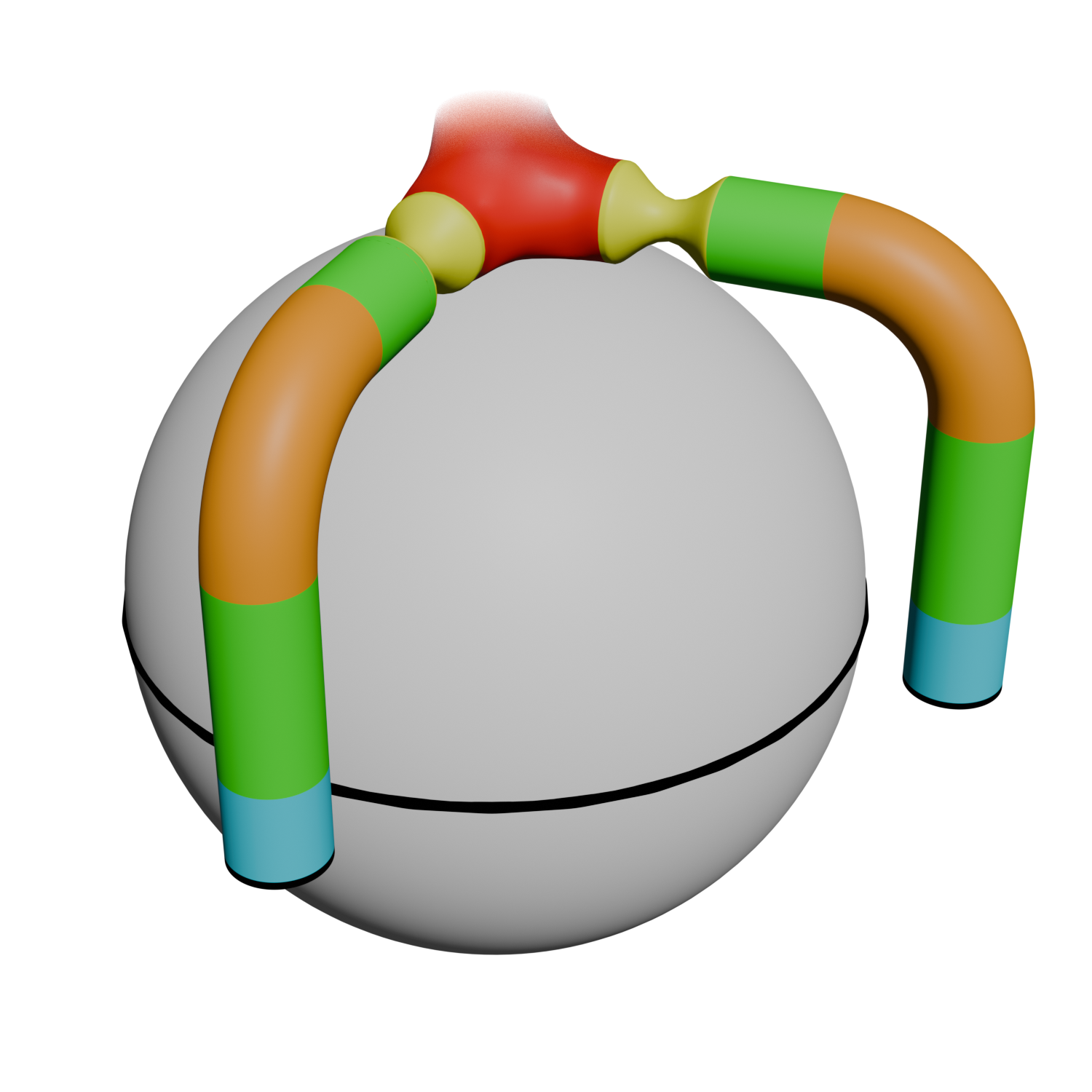
To embed the EP-complex $K(M)$ into a ball of constant radius (see Proposition 46) in $\mathbb{R}^{D}$ for $D=\mathcal{O}(m)$ , we construct it from isometric copies of different building blocks: circles, caps attaching to circles, triple junctions and three different types of L-arms connecting circles and triple junctions.

Refer to caption — Figure 3: A sphere with 4 holes and a cap attaching to circles corresponding to non-zero entries in their respective rows. Rows with more than 2 non-zero entries create triple junctions.

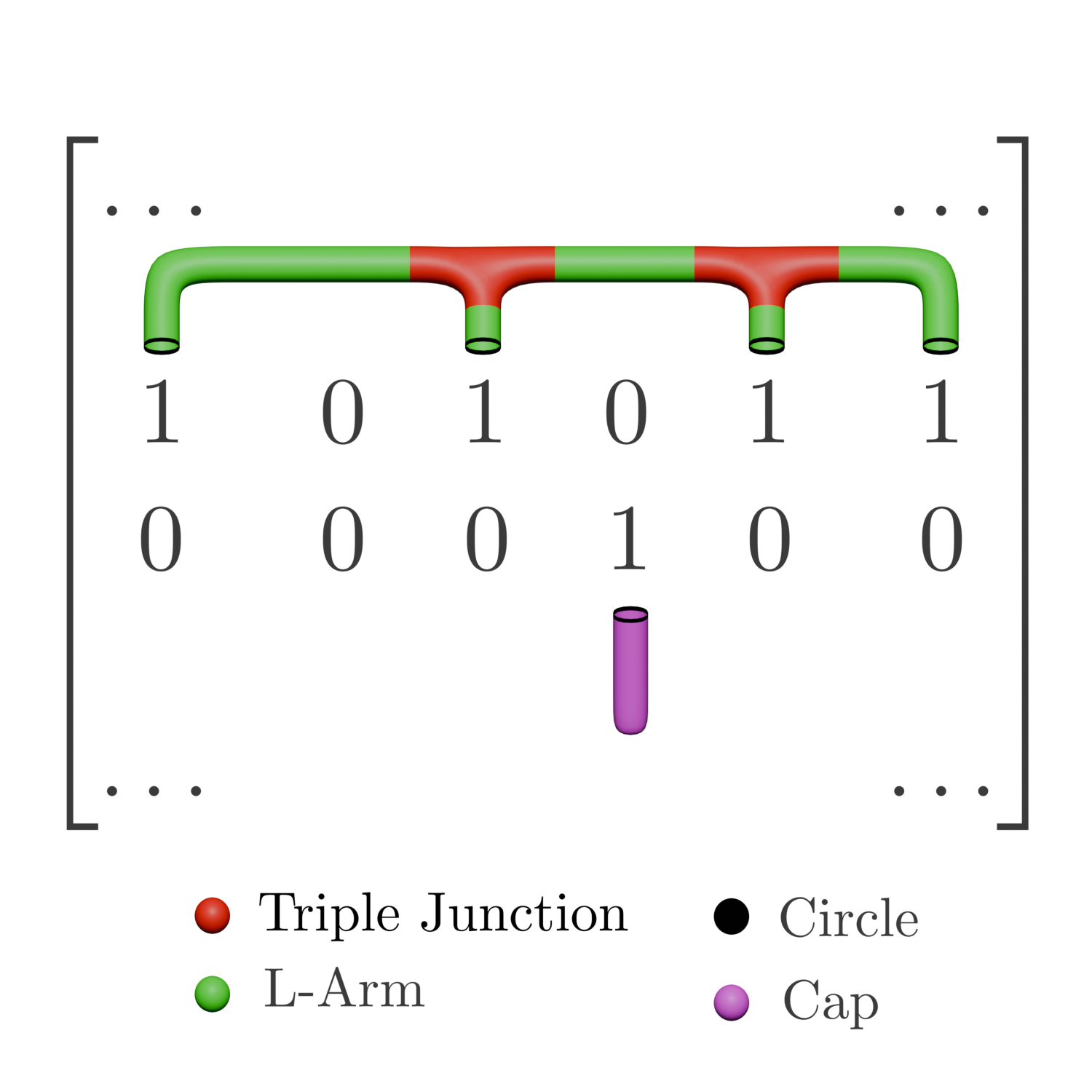
The idea is to embed each of the circles and triple junctions “in their own dimension”; this ensures they are far enough apart so that small $t$ -neighborhoods around them do not overlap. We then connect them with $L$ -arms. The precise construction is as follows.

1.

For each column of $M$ , add a (one-dimensional) circle $r_{0}\mathbb{S}^{1}$ of radius $r_{0}=1/10$ . For each circle, we add a dimension ( $\#\text{columns}$ (with non-zero entries) dimensions in total) and embed it centered at the coordinate vector $(0,\dots,0,1,0,\dots,0)^{\top}\in\mathbb{R}^{\#\text{columns}}$ . We also add 2 supplementary dimensions; each circle is oriented such that each of their tangent spaces (the 2D plane each is contained in) is spanned by these 2 extra dimensions.
2.
For each row, we consider different cases according to the number of non-zero entries.
- $\blacksquare$
  
  1 non-zero entry. Attach a cap to the circle pointing along a further dimension. The straight section of the cap has length $3r_{0}$ , and the half-sphere “on top” has radius $r_{0}$ .
- $\blacksquare$
  
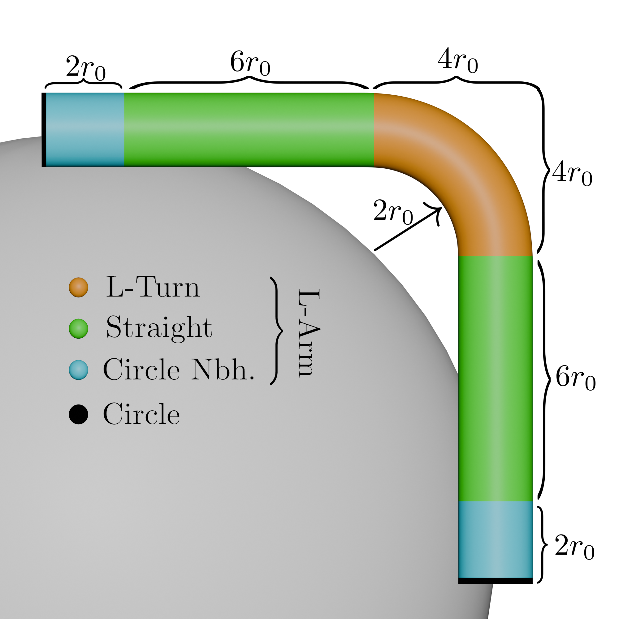
  2 non-zero entries. We add an L-arm connecting the two circles, traveling along the plane spanned by their 2 respective vectors; see the third image in Figure 4.
- $\blacksquare$
  
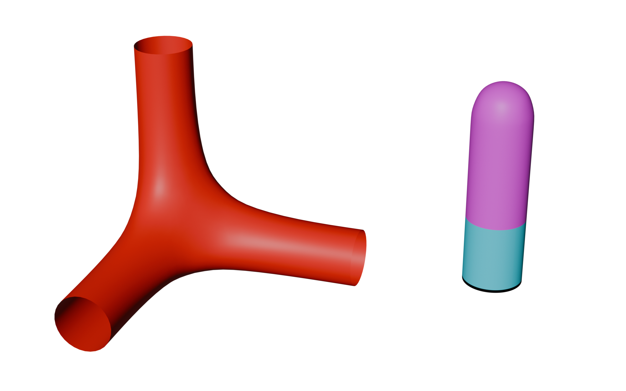
  $\geq 3$ non-zero entries. We add one dimension for each non-zero entry which is not the first or last non-zero entry of its row. For each such entry, we embed a triple junction centered at the unit vector associated to the added dimension, with its three arms pointing in directions tangent to $\mathbb{S}^{D-1}=\{x\in\mathbb{R}^{D}:\|x\|=1\}$ , towards the coordinate vectors specified by the circle corresponding to its column and the two adjacent – possibly separated by zeros – $1$ s in its row. An adjacent $1$ itself represents either a triple junction, or a circle associated to the column containing the first or last 1 in the row, as illustrated in Figure 3. The total number of dimensions is $\mathcal{O}(m)$ .
3.

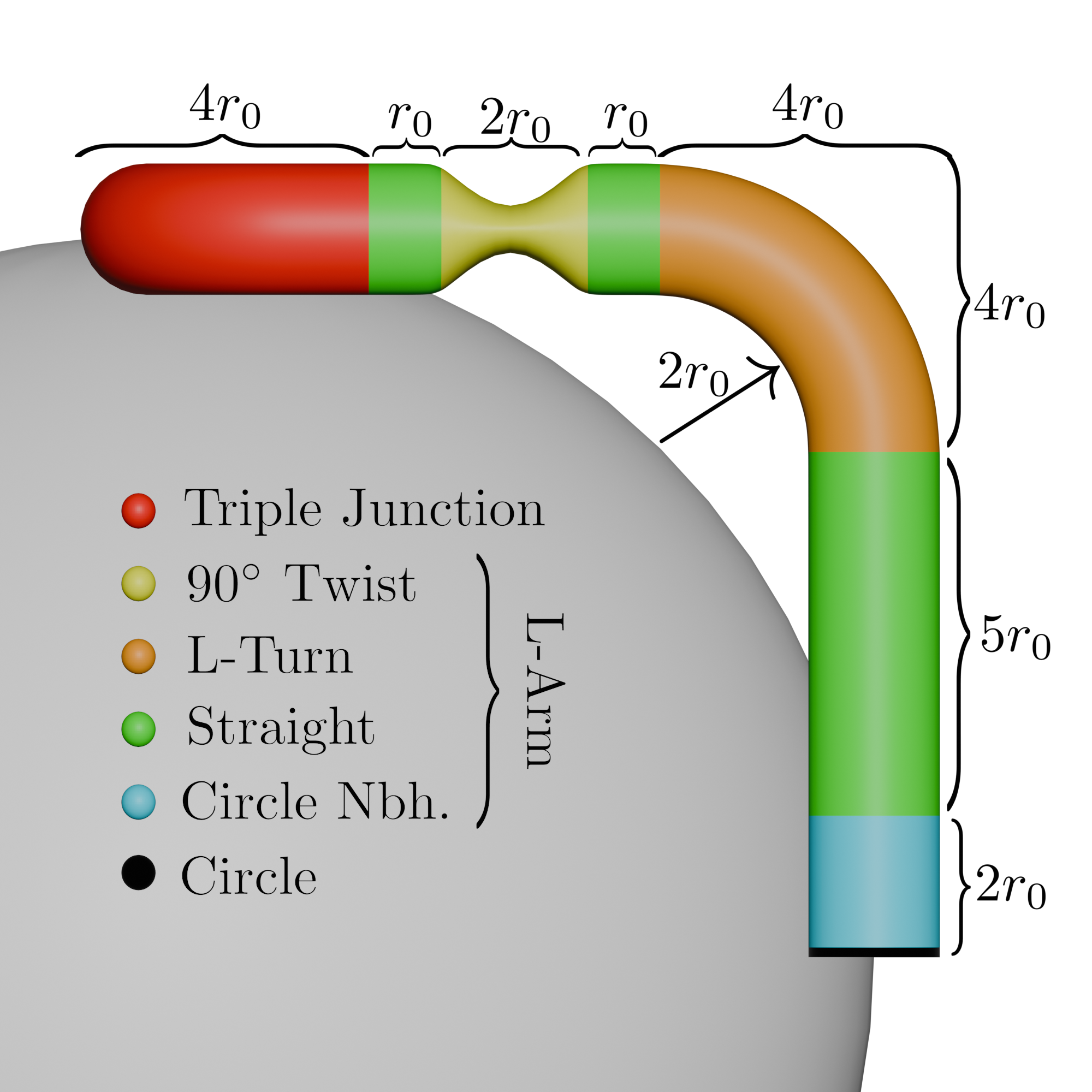
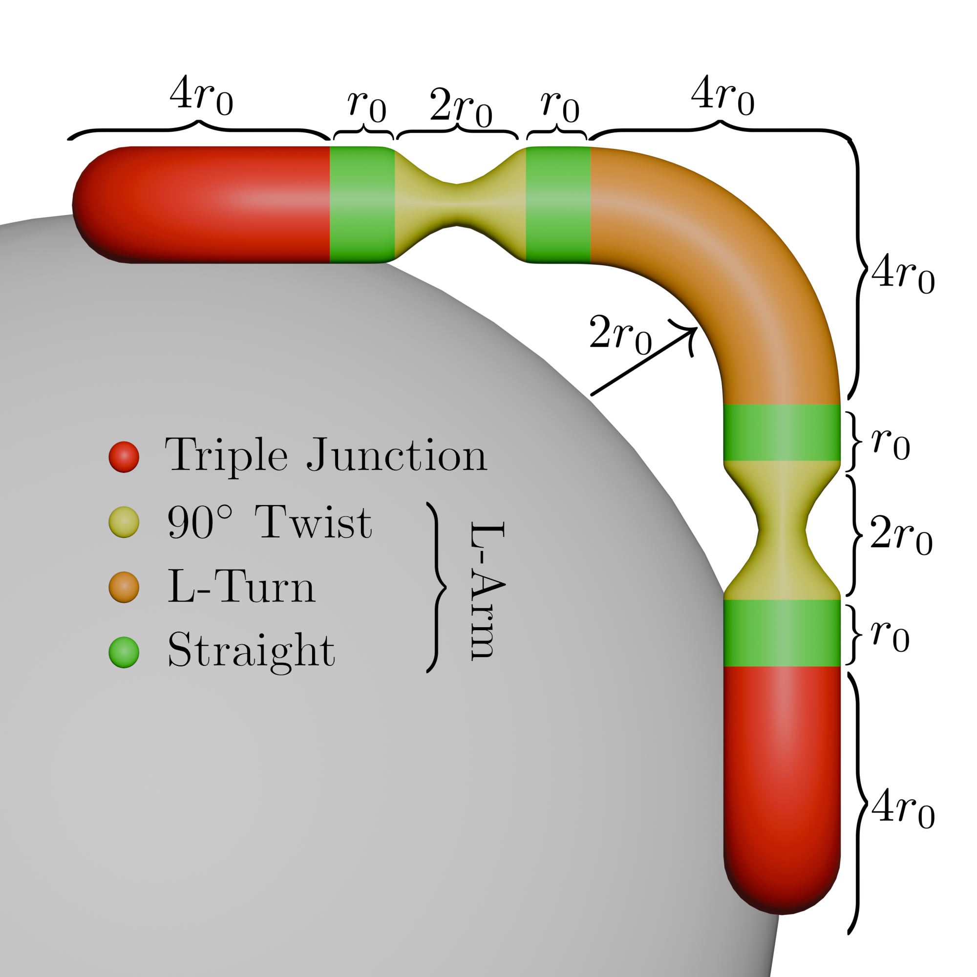
If a triple junction points towards another triple junction or a circle, we embed an L-arm connecting the two. These L-arms are homeomorphic to $\mathbb{S}^{1}\times[0,1]$ , and their anatomy is more precisely defined in Figure 4. The L-arms attaching to triple junctions include a twist to make the circle plane align with the boundary on the triple junction.

The complex $\mathcal{K}$ is homeomorphic to the EP complex, so $\dim H_{2}(\mathcal{K})=\dim((\operatorname*{im}M)^{\bot})$ [27].

While the embedding and the proofs for the multiplicative case are more involved, much of the reasoning is actually quite similar, albeit more technical. A first step is to ascertain that the geometry of $\mathcal{K}$ is simple enough to allow for good samples to be constructed.

Proposition 46.

Let $s>0$ , and $M$ a matrix with $m$ non-zero $\mathbb{F}_{2}$ -entries. Then

1.

A subset $\mathcal{S}\subseteq\mathcal{K}\subseteq\mathbb{R}^{D}$ of $\mathcal{O}(m/s^{2})$ points with $d_{H}(\mathcal{S},\mathcal{K})\leq s$ can be found in time $\mathcal{O}(m/s^{2})$ .
2.

The complex $\mathcal{K}$ admits a constant-time distance oracle and a diameter bound independent of $M$ .

Next, we need to make sure that the barcode of the VR-complex of the compact metric space $\mathcal{K}$ encodes its homology sufficiently well, and that approximations can recover the homology information of $\mathcal{K}$ .

Lemma 47.

Let $X\subseteq\mathbb{R}^{k}$ be an embedded metric space that admits a neighborhood deformation retraction $r:X^{t_{0}}\to X$ . Then, there are maps $\pi_{t}:|\textnormal{\v{C}}(X)_{t}|\to X$ ; $0<t\leq t_{0}$ , natural in $t$ that induce isomorphisms on all homology groups.

Lemma 48.

Let $X\subseteq\mathbb{R}^{k}$ be an embedded metric space. Suppose there is some $t_{0}>0$ such that for all $0<t\leq t_{0}$ we have maps $\pi_{t}:|\textnormal{\v{C}}(X)_{t}|\to X$ natural in $t$ that induce isomorphisms on homology groups. Then $|\operatorname{VR}(X)_{t/2}|\to|\textnormal{\v{C}}(X)_{t}|\xrightarrow{\pi_{t}}X$ induces isomorphisms on homology groups for all $t\leq t_{0}$ .

Proposition 49.

For a parameter $t_{0}>0$ that is independent of $M$ , there is a $t_{0}$ -neighborhood deformation retraction $\mathcal{K}^{t_{0}}\to\mathcal{K}$ of the embedded EP-complex $\mathcal{K}$ associated to $M$ .

Proof of Theorem 40.

Assume there is an $\varepsilon/2$ -approximation algorithm A for $\varepsilon<t_{0}/8$ , where $t_{0}>0$ is from Proposition 49. By Proposition 46, we obtain a finite metric space $\mathcal{S}$ with $d_{H}(\mathcal{S},\mathcal{K})\leq\varepsilon/2$ for the embedding $\mathcal{K}$ from Construction 1. Lemma 47 and Lemma 48 applied to the retraction from Proposition 49 yields an isomorphism of persistence modules

H_{2}(\operatorname{VR}(\mathcal{K})_{\bullet})|_{(0,t_{0}/2]}\xrightarrow{% \cong}\bigoplus_{\dim((\operatorname*{im}M)^{\bot})}\mathbbm{1}_{(0,t_{0}/2]},% \text{ with $\mathbbm{1}_{(0,t_{0}/2]}$ the interval module on $(0,t_{0}/2]$.}

By Hausdorff stability of the barcode (for compact metric spaces), we have

d_{I}\Big(H_{2}(\operatorname{VR}(\mathcal{S})_{\bullet})|_{(0,t_{0}/2]},% \bigoplus_{\dim((\operatorname*{im}M)^{\bot})}\mathbbm{1}_{(0,t_{0}/2]}\Big)% \leq\varepsilon/2<t_{0}/16\ .

By the triangle inequality, $d_{I}\Big({\textnormal{{A}}}(\mathcal{S})|_{(0,t_{0}/2]},\bigoplus_{\dim((% \operatorname*{im}M)^{\bot})}\mathbbm{1}_{(0,t_{0}/2]}\Big)\leq\varepsilon<t_{% 0}/8.$ As the inequality is strict, in the barcode of ${\textnormal{{A}}}(\mathcal{S})|_{(0,t_{0}/2]}$ there will be exactly $\dim((\operatorname*{im}M)^{\bot})$ many intervals of length strictly greater than $t_{0}/4$ , as any interval is only modified in length by at most $2\varepsilon<t_{0}/4$ . By Proposition 46, the construction of $\mathcal{S}$ takes $\mathcal{O}(m)$ time, and the evaluation ${\textnormal{{A}}}(\mathcal{S})$ is well-defined and takes $\mathcal{O}(m^{q})$ time, concluding the proof. $\hfill\blacktriangleleft$

5 On the hardness of multiplicative approximations

Oftentimes, a multiplicative definition of the interleaving distance and the resulting approximation of barcodes is better suited for certain applications, especially for multiscale analyses, e.g., of materials [37]. For multiplicative approximations, an algorithm taking $\tilde{\mathcal{O}}(|X|^{\omega})$ time (ignoring $\varepsilon$ -dependent factors) arises from the scheme in [50] in conjunction with the matrix multiplication time persistence algorithm in [43]. For large enough doubling dimension, Theorem 42 shows that improvement is unlikely.

$\blacktriangleright$ Remark 50.

The setting of Theorem 42 being that of metric spaces embedded in some $\mathbb{R}^{D}$ , the reasoning easily adapts to multiplicative approximations of barcodes of Čech complexes.

The proof of this theorem is very similar in spirit to the additive case: Embed the EP-complex $K=K(M)$ into Euclidean space $\mathbb{R}^{2d+3}$ , and extract its information about $\operatorname{rank}(M)$ from the barcode of a subsample $\mathcal{S}$ on its surface.

This time, as the size of the matrix $M$ increases, we cannot increase the embedding dimension, and there will intuitively be increasingly little space for the embedding $\mathcal{K}$ . We will thus only be able to prove an isomorphism

H_{2}(\operatorname{VR}(\mathcal{K})_{\bullet})_{(0,t_{m}]}\xrightarrow{\cong}% \bigoplus_{\dim((\operatorname*{im}M)^{\bot})}\mathbbm{1}_{(0,t_{m}]}

where $t_{m}=Cm^{-1/d}$ is dependent on the number of non-zero entries in $M$ . As the approximation algorithm A is multiplicative, and thus increasingly accurate on smaller scales $(0,s]$ , we will still be able to read the necessary information from the barcode of a sufficiently dense subsample $\mathcal{S}\subseteq K$ .

Here, we simply note that the construction of the complex for the multiplicative reduction harbors a number of technical challenges, since we need to find a way to navigate different sections of the constructed geometric complex efficiently, striking a compromise between keeping points of the complex sufficiently far apart in the embedding, while also packing them closely enough so that navigating the complex is not too computationally expensive. The multiplicative hardness then follows in essentially the same way as the additive case, by combining the additive approximation from subsampling with multiplicative approximations.

6 Discussion

In this paper, we showed both 1) upper bounds on the complexity of computing additive approximations to invariants of persistence modules under simple geometric assumptions on the underlying metric space and 2) a reduction from matrix rank to approximations of barcodes of the VR or Čech filtration, giving rise to lower bounds on approximations for barcodes in the absence of these assumptions. The upper bounds we show are significant in two ways. In the multiparameter setting, they are the first of their kind, showing that invariants of the measure bifiltration on doubling spaces with bounded diameter can be analyzed probabilistically through uniform samples of size independent of the number of input points. In the one-parameter setting, our results give rise to a recognizable barrier between regimes where multiplicative approximations are feasible and those where the number of points is large enough that an additive approximation of stable barcodes becomes easier to compute.

Our lower bounds show that such a distinction of different regimes is meaningful, as multiplicative approximations are generally expensive to compute, and additive approximations become so for a sufficiently exact approximation quality and with no control over the doubling dimension.

Our results raise the following natural follow-up questions.

1.

What is the practical relevance of the upper bounds derived in the first part of the paper? Can an algorithm engineering approach be used for performance gains over state-of-the-art implementations, or are the algorithms of a purely theoretical nature?
2.

Are there geometrically informative filtrations whose (stable) barcode can be approximated more efficiently than the VR or Čech filtrations?
3.

Are there other multifiltrations that allow computational improvements over the 1-parameter case?
4.

Can the barcode of the VR or Čech filtration be approximated more effectively if one only seeks a partial approximation, say, of the $k$ longest intervals? Note for this that the spectral sequence algorithm [28] can be used to achieve the converse: To probe the homological features in order of nondecreasing persistence.

References

[1] Michał Adamaszek and Juraj Stacho. Complexity of simplicial homology and independence complexes of chordal graphs. Computational Geometry, 57:8–18, 2016. doi:10.1016/j.comgeo.2016.05.003.
[2] Henry Adams and Žiga Virk. Lower Bounds on the Homology of Vietoris–Rips Complexes of Hypercube Graphs. Bulletin of the Malaysian Mathematical Sciences Society, 47(3):72, 2024. doi:10.1007/s40840-024-01663-x.
[3] Ángel Javier Alonso. A Sparse Multicover Bifiltration of Linear Size. In Oswin Aichholzer and Haitao Wang, editors, 41st International Symposium on Computational Geometry (SoCG 2025), volume 332 of Leibniz International Proceedings in Informatics (LIPIcs), pages 6:1—-6:18, Dagstuhl, Germany, 2025. Schloss Dagstuhl – Leibniz-Zentrum für Informatik. doi:10.4230/LIPIcs.SoCG.2025.6.
[4] Simon Apers, Sander Gribling, Sayantan Sen, and Dániel Szabó. A (simple) classical algorithm for estimating Betti numbers. Quantum, 7:1202, December 2023. doi:10.22331/q-2023-12-06-1202.
[5] Ulrich Bauer and Herbert Edelsbrunner. The Morse theory of Čech and Delaunay complexes. Transactions of the American Mathematical Society, 369(5):3741–3762, December 2016. doi:10.1090/tran/6991.
[6] Ulrich Bauer, Michael Kerber, and Jan Reininghaus. Clear and Compress: Computing Persistent Homology in Chunks. In Peer-Timo Bremer, Ingrid Hotz, Valerio Pascucci, and Ronald Peikert, editors, Topological Methods in Data Analysis and Visualization III, pages 103–117, Cham, 2014. Springer International Publishing. doi:10.1007/978-3-319-04099-8_7.
[7] Ulrich Bauer and Fabian Roll. Wrapping Cycles in Delaunay Complexes: Bridging Persistent Homology and Discrete Morse Theory. In Wolfgang Mulzer and Jeff M. Phillips, editors, 40th International Symposium on Computational Geometry (SoCG 2024), volume 293 of Leibniz International Proceedings in Informatics (LIPIcs), pages 15:1–15:16, Dagstuhl, Germany, 2024. Schloss Dagstuhl – Leibniz-Zentrum für Informatik. doi:10.4230/LIPIcs.SoCG.2024.15.
[8] Jacob Billings, Manish Saggar, Jaroslav Hlinka, Shella Keilholz, and Giovanni Petri. Simplicial and topological descriptions of human brain dynamics. Network Neuroscience, 5(2):549–568, June 2021. doi:10.1162/netn_a_00190.
[9] Patrick Billingsley. Convergence of Probability Measures. John Wiley & Sons, New York, second edition, 1999.
[10] Andrew J Blumberg and Michael Lesnick. Stability of 2-Parameter Persistent Homology. Foundations of Computational Mathematics, 24(2):385–427, April 2024. doi:10.1007/s10208-022-09576-6.
[11] Mickaël Buchet, Bianca B. Dornelas, and Michael Kerber. Sparse Higher Order Čech Filtrations. In Erin W Chambers and Joachim Gudmundsson, editors, 39th International Symposium on Computational Geometry (SoCG 2023), volume 258 of Leibniz International Proceedings in Informatics (LIPIcs), pages 20:1—-20:17, Dagstuhl, Germany, 2023. Schloss Dagstuhl – Leibniz-Zentrum für Informatik. doi:10.4230/LIPIcs.SoCG.2023.20.
[12] Mickaël Buchet, Frédéric Chazal, Steve Y Oudot, and Donald R Sheehy. Efficient and robust persistent homology for measures. Computational Geometry, 58:70–96, 2016. doi:10.1016/j.comgeo.2016.07.001.
[13] Gunnar Carlsson. Topology and data. Bulletin of the American Mathematical Society, 46(2):255–308, January 2009. doi:10.1090/S0273-0979-09-01249-X.
[14] W. Chachólski, M. Scolamiero, and F. Vaccarino. Combinatorial presentation of multidimensional persistent homology. Journal of Pure and Applied Algebra, 221(5):1055–1075, 2017. doi:10.1016/j.jpaa.2016.09.001.
[15] Frédéric Chazal, Vin de Silva, and Steve Oudot. Persistence stability for geometric complexes. Geometriae Dedicata, 173(1):193–214, 2014. doi:10.1007/s10711-013-9937-z.
[16] Frederic Chazal, Brittany Fasy, Fabrizio Lecci, Bertrand Michel, Alessandro Rinaldo, and Larry Wasserman. Subsampling Methods for Persistent Homology. In Francis Bach and David Blei, editors, Proceedings of the 32nd International Conference on Machine Learning, volume 37 of Proceedings of Machine Learning Research, pages 2143–2151, Lille, France, 2015. PMLR. URL: https://proceedings.mlr.press/v37/chazal15.html.
[17] Oliver Chubet, Don Sheehy, and Siddharth Sheth. Simple Construction of Greedy Trees and Greedy Permutations. arXiv preprint, pages 1–27, 2024. doi:10.48550/arXiv.2412.02554.
[18] Kenneth L. Clarkson. Nearest neighbor searching in metric spaces: Experimental results for sb(s). Technical report, Bell Laboratories, 2002. URL: https://kenclarkson.org/Msb/white_paper.pdf.
[19] Jacobus Conradi, Anne Driemel, and Benedikt Kolbe. (1+ $\epsilon$ )–ANN Data Structure for Curves via Subspaces of Bounded Doubling Dimension. Computing in Geometry and Topology, 3(2):1–22, 2024. doi:10.57717/cgt.v3i2.45.
[20] René Corbet, Michael Kerber, Michael Lesnick, and Georg Osang. Computing the Multicover Bifiltration. Discrete & Computational Geometry, 70(2):376–405, 2023. doi:10.1007/s00454-022-00476-8.
[21] René Corbet, Michael Kerber, Michael Lesnick, and Georg Osang. Computing the multicover bifiltration, 2022. arXiv:2103.07823.
[22] Daniel Dadush, Cristóbal Guzmán, and Neil Olver. Fast, Deterministic and Sparse Dimensionality Reduction, pages 1330–1344. Society for Industrial and Applied Mathematics, Philadelphia, PA, 2018. doi:10.1137/1.9781611975031.87.
[23] Vin De Silva and Gunnar Carlsson. Topological estimation using witness complexes. In Proceedings of the First Eurographics Conference on Point-Based Graphics, SPBG’04, pages 157–166, Goslar, DEU, 2004. Eurographics Association. doi:10.2312/SPBG/SPBG04/157-166.
[24] Vin de Silva and Robert Ghrist. Coverage in sensor networks via persistent homology. Algebraic & Geometric Topology, 7(1):339–358, April 2007. doi:10.2140/agt.2007.7.339.
[25] Tamal K Dey, Fengtao Fan, and Yusu Wang. Graph induced complex on point data. Computational Geometry, 48(8):575–588, 2015. doi:10.1016/j.comgeo.2015.04.003.
[26] R. M. Dudley. The Speed of Mean Glivenko-Cantelli Convergence. Ann. Math. Statist., 40(6):40–50, 1969. URL: http://dml.mathdoc.fr/item/1177697802.
[27] H. Edelsbrunner and S. Parsa. On the computational complexity of Betti numbers: reductions from matrix rank. In Proceedings of the Twenty-Fifth Annual ACM-SIAM Symposium on Discrete Algorithms, SODA ’14, pages 152–160, USA, 2014. Society for Industrial and Applied Mathematics.
[28] Herbert Edelsbrunner and John L. Harer. Computational Topology: An Introduction. American Mathematical Society, 2010.
[29] Herbert Edelsbrunner, David Letscher, and Afra Zomorodian. Topological persistence and simplification. Discrete and Computational Geometry, 28(4):511–533, 2002. doi:10.1007/s00454-002-2885-2.
[30] Anass B El-Yaagoubi, Moo K Chung, and Hernando Ombao. Topological Data Analysis for Multivariate Time Series Data. Entropy, 25(11), 2023. doi:10.3390/e25111509.
[31] David Eppstein, Sariel Har-Peled, and Anastasios Sidiropoulos. Approximate greedy clustering and distance selection for graph metrics. Journal of Computational Geometry, 11(1):629–652, 2020. doi:10.20382/jocg.v11i1a25.
[32] Guillin Fournier. On the rate of convergence in Wasserstein distance of the empirical measure. Probability Theory and Related Fields, 2015. doi:10.1007/s00440-014-0583-7.
[33] Marcio Gameiro, Yasuaki Hiraoka, Shunsuke Izumi, Miroslav Kramar, Konstantin Mischaikow, and Vidit Nanda. A topological measurement of protein compressibility. Japan Journal of Industrial and Applied Mathematics, 32(1):1–17, 2015. doi:10.1007/s13160-014-0153-5.
[34] Teofilo F. Gonzalez. Clustering to minimize the maximum intercluster distance. Theoretical Computer Science, 38:293–306, 1985. doi:10.1016/0304-3975(85)90224-5.
[35] Sariel Har-Peled and Manor Mendel. Fast construction of nets in low dimensional metrics, and their applications. In Proceedings of the Twenty-First Annual Symposium on Computational Geometry, SCG ’05, pages 150–158, New York, NY, USA, 2005. Association for Computing Machinery. doi:10.1145/1064092.1064117.
[36] Maria Herick, Michael Joachim, and Jan Vahrenhold. Adaptive approximation of persistent homology. Journal of Applied and Computational Topology, 8(8):2327–2366, December 2024. doi:10.1007/s41468-024-00192-7.
[37] Yasuaki Hiraoka, Takenobu Nakamura, Akihiko Hirata, Emerson G. Escolar, Kaname Matsue, and Yasumasa Nishiura. Hierarchical structures of amorphous solids characterized by persistent homology. Proceedings of the National Academy of Sciences, 113(26):7035–7040, 2016. doi:10.1073/pnas.1520877113.
[38] Dorit S. Hochbaum and David B. Shmoys. A best possible heuristic for the k-center problem. Math. Oper. Res., 10(2):180–184, 1985. doi:10.1287/moor.10.2.180.
[39] Christoph Hofer, Roland Kwitt, Marc Niethammer, and Andreas Uhl. Deep learning with topological signatures. In Proceedings of the 31st International Conference on Neural Information Processing Systems, NIPS’17, pages 1633–1643, Red Hook, NY, USA, 2017. Curran Associates Inc.
[40] Violeta Kovacev-Nikolic, Peter Bubenik, Dragan Nikolić, and Giseon Heo. Using persistent homology and dynamical distances to analyze protein binding. Statistical applications in genetics and molecular biology, 15(1):19–38, March 2016. doi:10.1515/sagmb-2015-0057.
[41] Michael Lesnick and Matthew Wright. Computing Minimal Presentations and Bigraded Betti Numbers of 2-Parameter Persistent Homology. SIAM Journal on Applied Algebra and Geometry, 6(2):267–298, 2022. doi:10.1137/20M1388425.
[42] David Loiseaux, Mathieu Carrière, and Andrew J. Blumberg. A framework for fast and stable representations of multiparameter persistent homology decompositions. In Proceedings of the 37th International Conference on Neural Information Processing Systems, NIPS ’23, Red Hook, NY, USA, 2023. Curran Associates Inc.
[43] Dmitriy Morozov and Primoz Skraba. Persistent (Co)Homology in Matrix Multiplication Time. In Oswin Aichholzer and Haitao Wang, editors, 41st International Symposium on Computational Geometry (SoCG 2025), volume 332 of Leibniz International Proceedings in Informatics (LIPIcs), pages 68:1–68:16, Dagstuhl, Germany, 2025. Schloss Dagstuhl – Leibniz-Zentrum für Informatik. doi:10.4230/LIPIcs.SoCG.2025.68.
[44] Nina Otter, Mason A Porter, Ulrike Tillmann, Peter Grindrod, and Heather A Harrington. A roadmap for the computation of persistent homology. EPJ Data Science, 6(1):17, 2017. doi:10.1140/epjds/s13688-017-0109-5.
[45] Steve Oudot. Persistence Theory: From Quiver Representations to Data Analysis, volume 209. American Mathematical Society, 2015.
[46] Jan Reininghaus, Stefan Huber, Ulrich Bauer, and Roland Kwitt. A stable multi-scale kernel for topological machine learning. In 2015 IEEE Conference on Computer Vision and Pattern Recognition (CVPR), pages 4741–4748, 2015. doi:10.1109/CVPR.2015.7299106.
[47] Vanessa Robins and Katharine Turner. Principal component analysis of persistent homology rank functions with case studies of spatial point patterns, sphere packing and colloids. Physica D: Nonlinear Phenomena, 334:99–117, 2016. doi:10.1016/j.physd.2016.03.007.
[48] Sara Scaramuccia, Federico Iuricich, Leila De Floriani, and Claudia Landi. Computing multiparameter persistent homology through a discrete Morse-based approach. Computational Geometry, 89:101623, August 2020. doi:10.1016/j.comgeo.2020.101623.
[49] Alexander Schmidhuber and Seth Lloyd. Complexity-theoretic limitations on quantum algorithms for topological data analysis. PRX Quantum, 4:040349, December 2023. doi:10.1103/PRXQuantum.4.040349.
[50] Donald R. Sheehy. Linear-Size Approximations to the Vietoris–Rips Filtration. Discrete & Computational Geometry, 49(4):778–796, June 2013. doi:10.1007/s00454-013-9513-1.
[51] Donald R. Sheehy. The Persistent Homology of Distance Functions under Random Projection. In Proceedings of the thirtieth annual symposium on Computational geometry, pages 328–334, New York, NY, USA, June 2014. ACM. doi:10.1145/2582112.2582126.
[52] Donald R. Sheehy. A Sparse Delaunay Filtration. In Kevin Buchin and Éric Colin de Verdière, editors, 37th International Symposium on Computational Geometry (SoCG 2021), volume 189 of Leibniz International Proceedings in Informatics (LIPIcs), pages 58:1–58:16, Dagstuhl, Germany, 2021. Schloss Dagstuhl – Leibniz-Zentrum für Informatik. doi:10.4230/LIPIcs.SoCG.2021.58.
[53] Donald R. Sheehy and Siddharth Sheth. Sketching persistence diagrams, 2021. doi:10.4230/LIPIcs.SoCG.2021.57.
[54] T. Sousbie. The persistent cosmic web and its filamentary structure – i. theory and implementation. Monthly Notices of the Royal Astronomical Society, 414(1):350–383, 2011. doi:10.1111/j.1365-2966.2011.18394.x.
[55] Katharine Turner, Yuriy Mileyko, Sayan Mukherjee, and John Harer. Fréchet Means for Distributions of Persistence Diagrams. Discrete and Computational Geometry, 52(1):44–70, 2014. doi:10.1007/s00454-014-9604-7.
[56] Jonathan Weed and Francis Bach. Sharp asymptotic and finite-sample rates of convergence of empirical measures in Wasserstein distance, 2017. arXiv:1707.00087.
[57] Afra Zomorodian and Gunnar Carlsson. Computing Persistent Homology. Discrete & Computational Geometry, 33(2):249–274, 2005. doi:10.1007/s00454-004-1146-y.

[bib.bib1] [1] Michał Adamaszek and Juraj Stacho. Complexity of simplicial homology and independence complexes of chordal graphs. Computational Geometry, 57:8–18, 2016. doi:10.1016/j.comgeo.2016.05.003.

[bib.bib2] [2] Henry Adams and Žiga Virk. Lower Bounds on the Homology of Vietoris–Rips Complexes of Hypercube Graphs. Bulletin of the Malaysian Mathematical Sciences Society, 47(3):72, 2024. doi:10.1007/s40840-024-01663-x.

[bib.bib3] [3] Ángel Javier Alonso. A Sparse Multicover Bifiltration of Linear Size. In Oswin Aichholzer and Haitao Wang, editors, 41st International Symposium on Computational Geometry (SoCG 2025), volume 332 of Leibniz International Proceedings in Informatics (LIPIcs), pages 6:1—-6:18, Dagstuhl, Germany, 2025. Schloss Dagstuhl – Leibniz-Zentrum für Informatik. doi:10.4230/LIPIcs.SoCG.2025.6.

[bib.bib4] [4] Simon Apers, Sander Gribling, Sayantan Sen, and Dániel Szabó. A (simple) classical algorithm for estimating Betti numbers. Quantum, 7:1202, December 2023. doi:10.22331/q-2023-12-06-1202.

[bib.bib5] [5] Ulrich Bauer and Herbert Edelsbrunner. The Morse theory of Čech and Delaunay complexes. Transactions of the American Mathematical Society, 369(5):3741–3762, December 2016. doi:10.1090/tran/6991.

[bib.bib6] [6] Ulrich Bauer, Michael Kerber, and Jan Reininghaus. Clear and Compress: Computing Persistent Homology in Chunks. In Peer-Timo Bremer, Ingrid Hotz, Valerio Pascucci, and Ronald Peikert, editors, Topological Methods in Data Analysis and Visualization III, pages 103–117, Cham, 2014. Springer International Publishing. doi:10.1007/978-3-319-04099-8_7.

[bib.bib7] [7] Ulrich Bauer and Fabian Roll. Wrapping Cycles in Delaunay Complexes: Bridging Persistent Homology and Discrete Morse Theory. In Wolfgang Mulzer and Jeff M. Phillips, editors, 40th International Symposium on Computational Geometry (SoCG 2024), volume 293 of Leibniz International Proceedings in Informatics (LIPIcs), pages 15:1–15:16, Dagstuhl, Germany, 2024. Schloss Dagstuhl – Leibniz-Zentrum für Informatik. doi:10.4230/LIPIcs.SoCG.2024.15.

[bib.bib8] [8] Jacob Billings, Manish Saggar, Jaroslav Hlinka, Shella Keilholz, and Giovanni Petri. Simplicial and topological descriptions of human brain dynamics. Network Neuroscience, 5(2):549–568, June 2021. doi:10.1162/netn_a_00190.

[bib.bib9] [9] Patrick Billingsley. Convergence of Probability Measures. John Wiley & Sons, New York, second edition, 1999.

[bib.bib10] [10] Andrew J Blumberg and Michael Lesnick. Stability of 2-Parameter Persistent Homology. Foundations of Computational Mathematics, 24(2):385–427, April 2024. doi:10.1007/s10208-022-09576-6.

[bib.bib11] [11] Mickaël Buchet, Bianca B. Dornelas, and Michael Kerber. Sparse Higher Order Čech Filtrations. In Erin W Chambers and Joachim Gudmundsson, editors, 39th International Symposium on Computational Geometry (SoCG 2023), volume 258 of Leibniz International Proceedings in Informatics (LIPIcs), pages 20:1—-20:17, Dagstuhl, Germany, 2023. Schloss Dagstuhl – Leibniz-Zentrum für Informatik. doi:10.4230/LIPIcs.SoCG.2023.20.

[bib.bib12] [12] Mickaël Buchet, Frédéric Chazal, Steve Y Oudot, and Donald R Sheehy. Efficient and robust persistent homology for measures. Computational Geometry, 58:70–96, 2016. doi:10.1016/j.comgeo.2016.07.001.

[bib.bib13] [13] Gunnar Carlsson. Topology and data. Bulletin of the American Mathematical Society, 46(2):255–308, January 2009. doi:10.1090/S0273-0979-09-01249-X.

[bib.bib14] [14] W. Chachólski, M. Scolamiero, and F. Vaccarino. Combinatorial presentation of multidimensional persistent homology. Journal of Pure and Applied Algebra, 221(5):1055–1075, 2017. doi:10.1016/j.jpaa.2016.09.001.

[bib.bib15] [15] Frédéric Chazal, Vin de Silva, and Steve Oudot. Persistence stability for geometric complexes. Geometriae Dedicata, 173(1):193–214, 2014. doi:10.1007/s10711-013-9937-z.

[bib.bib16] [16] Frederic Chazal, Brittany Fasy, Fabrizio Lecci, Bertrand Michel, Alessandro Rinaldo, and Larry Wasserman. Subsampling Methods for Persistent Homology. In Francis Bach and David Blei, editors, Proceedings of the 32nd International Conference on Machine Learning, volume 37 of Proceedings of Machine Learning Research, pages 2143–2151, Lille, France, 2015. PMLR. URL: https://proceedings.mlr.press/v37/chazal15.html.

[bib.bib17] [17] Oliver Chubet, Don Sheehy, and Siddharth Sheth. Simple Construction of Greedy Trees and Greedy Permutations. arXiv preprint, pages 1–27, 2024. doi:10.48550/arXiv.2412.02554.

[bib.bib18] [18] Kenneth L. Clarkson. Nearest neighbor searching in metric spaces: Experimental results for sb(s). Technical report, Bell Laboratories, 2002. URL: https://kenclarkson.org/Msb/white_paper.pdf.

[bib.bib19] [19] Jacobus Conradi, Anne Driemel, and Benedikt Kolbe. (1+ $\epsilon$ )–ANN Data Structure for Curves via Subspaces of Bounded Doubling Dimension. Computing in Geometry and Topology, 3(2):1–22, 2024. doi:10.57717/cgt.v3i2.45.

[bib.bib20] [20] René Corbet, Michael Kerber, Michael Lesnick, and Georg Osang. Computing the Multicover Bifiltration. Discrete & Computational Geometry, 70(2):376–405, 2023. doi:10.1007/s00454-022-00476-8.

[bib.bib21] [21] René Corbet, Michael Kerber, Michael Lesnick, and Georg Osang. Computing the multicover bifiltration, 2022. arXiv:2103.07823.

[bib.bib22] [22] Daniel Dadush, Cristóbal Guzmán, and Neil Olver. Fast, Deterministic and Sparse Dimensionality Reduction, pages 1330–1344. Society for Industrial and Applied Mathematics, Philadelphia, PA, 2018. doi:10.1137/1.9781611975031.87.

[bib.bib23] [23] Vin De Silva and Gunnar Carlsson. Topological estimation using witness complexes. In Proceedings of the First Eurographics Conference on Point-Based Graphics, SPBG’04, pages 157–166, Goslar, DEU, 2004. Eurographics Association. doi:10.2312/SPBG/SPBG04/157-166.

[bib.bib24] [24] Vin de Silva and Robert Ghrist. Coverage in sensor networks via persistent homology. Algebraic & Geometric Topology, 7(1):339–358, April 2007. doi:10.2140/agt.2007.7.339.

[bib.bib25] [25] Tamal K Dey, Fengtao Fan, and Yusu Wang. Graph induced complex on point data. Computational Geometry, 48(8):575–588, 2015. doi:10.1016/j.comgeo.2015.04.003.

[bib.bib26] [26] R. M. Dudley. The Speed of Mean Glivenko-Cantelli Convergence. Ann. Math. Statist., 40(6):40–50, 1969. URL: http://dml.mathdoc.fr/item/1177697802.

[bib.bib27] [27] H. Edelsbrunner and S. Parsa. On the computational complexity of Betti numbers: reductions from matrix rank. In Proceedings of the Twenty-Fifth Annual ACM-SIAM Symposium on Discrete Algorithms, SODA ’14, pages 152–160, USA, 2014. Society for Industrial and Applied Mathematics.

[bib.bib28] [28] Herbert Edelsbrunner and John L. Harer. Computational Topology: An Introduction. American Mathematical Society, 2010.

[bib.bib29] [29] Herbert Edelsbrunner, David Letscher, and Afra Zomorodian. Topological persistence and simplification. Discrete and Computational Geometry, 28(4):511–533, 2002. doi:10.1007/s00454-002-2885-2.

[bib.bib30] [30] Anass B El-Yaagoubi, Moo K Chung, and Hernando Ombao. Topological Data Analysis for Multivariate Time Series Data. Entropy, 25(11), 2023. doi:10.3390/e25111509.

[bib.bib31] [31] David Eppstein, Sariel Har-Peled, and Anastasios Sidiropoulos. Approximate greedy clustering and distance selection for graph metrics. Journal of Computational Geometry, 11(1):629–652, 2020. doi:10.20382/jocg.v11i1a25.

[bib.bib32] [32] Guillin Fournier. On the rate of convergence in Wasserstein distance of the empirical measure. Probability Theory and Related Fields, 2015. doi:10.1007/s00440-014-0583-7.

[bib.bib33] [33] Marcio Gameiro, Yasuaki Hiraoka, Shunsuke Izumi, Miroslav Kramar, Konstantin Mischaikow, and Vidit Nanda. A topological measurement of protein compressibility. Japan Journal of Industrial and Applied Mathematics, 32(1):1–17, 2015. doi:10.1007/s13160-014-0153-5.

[bib.bib34] [34] Teofilo F. Gonzalez. Clustering to minimize the maximum intercluster distance. Theoretical Computer Science, 38:293–306, 1985. doi:10.1016/0304-3975(85)90224-5.

[bib.bib35] [35] Sariel Har-Peled and Manor Mendel. Fast construction of nets in low dimensional metrics, and their applications. In Proceedings of the Twenty-First Annual Symposium on Computational Geometry, SCG ’05, pages 150–158, New York, NY, USA, 2005. Association for Computing Machinery. doi:10.1145/1064092.1064117.

[bib.bib36] [36] Maria Herick, Michael Joachim, and Jan Vahrenhold. Adaptive approximation of persistent homology. Journal of Applied and Computational Topology, 8(8):2327–2366, December 2024. doi:10.1007/s41468-024-00192-7.

[bib.bib37] [37] Yasuaki Hiraoka, Takenobu Nakamura, Akihiko Hirata, Emerson G. Escolar, Kaname Matsue, and Yasumasa Nishiura. Hierarchical structures of amorphous solids characterized by persistent homology. Proceedings of the National Academy of Sciences, 113(26):7035–7040, 2016. doi:10.1073/pnas.1520877113.

[bib.bib38] [38] Dorit S. Hochbaum and David B. Shmoys. A best possible heuristic for the k-center problem. Math. Oper. Res., 10(2):180–184, 1985. doi:10.1287/moor.10.2.180.

[bib.bib39] [39] Christoph Hofer, Roland Kwitt, Marc Niethammer, and Andreas Uhl. Deep learning with topological signatures. In Proceedings of the 31st International Conference on Neural Information Processing Systems, NIPS’17, pages 1633–1643, Red Hook, NY, USA, 2017. Curran Associates Inc.

[bib.bib40] [40] Violeta Kovacev-Nikolic, Peter Bubenik, Dragan Nikolić, and Giseon Heo. Using persistent homology and dynamical distances to analyze protein binding. Statistical applications in genetics and molecular biology, 15(1):19–38, March 2016. doi:10.1515/sagmb-2015-0057.

[bib.bib41] [41] Michael Lesnick and Matthew Wright. Computing Minimal Presentations and Bigraded Betti Numbers of 2-Parameter Persistent Homology. SIAM Journal on Applied Algebra and Geometry, 6(2):267–298, 2022. doi:10.1137/20M1388425.

[bib.bib42] [42] David Loiseaux, Mathieu Carrière, and Andrew J. Blumberg. A framework for fast and stable representations of multiparameter persistent homology decompositions. In Proceedings of the 37th International Conference on Neural Information Processing Systems, NIPS ’23, Red Hook, NY, USA, 2023. Curran Associates Inc.

[bib.bib43] [43] Dmitriy Morozov and Primoz Skraba. Persistent (Co)Homology in Matrix Multiplication Time. In Oswin Aichholzer and Haitao Wang, editors, 41st International Symposium on Computational Geometry (SoCG 2025), volume 332 of Leibniz International Proceedings in Informatics (LIPIcs), pages 68:1–68:16, Dagstuhl, Germany, 2025. Schloss Dagstuhl – Leibniz-Zentrum für Informatik. doi:10.4230/LIPIcs.SoCG.2025.68.

[bib.bib44] [44] Nina Otter, Mason A Porter, Ulrike Tillmann, Peter Grindrod, and Heather A Harrington. A roadmap for the computation of persistent homology. EPJ Data Science, 6(1):17, 2017. doi:10.1140/epjds/s13688-017-0109-5.

[bib.bib45] [45] Steve Oudot. Persistence Theory: From Quiver Representations to Data Analysis, volume 209. American Mathematical Society, 2015.

[bib.bib46] [46] Jan Reininghaus, Stefan Huber, Ulrich Bauer, and Roland Kwitt. A stable multi-scale kernel for topological machine learning. In 2015 IEEE Conference on Computer Vision and Pattern Recognition (CVPR), pages 4741–4748, 2015. doi:10.1109/CVPR.2015.7299106.

[bib.bib47] [47] Vanessa Robins and Katharine Turner. Principal component analysis of persistent homology rank functions with case studies of spatial point patterns, sphere packing and colloids. Physica D: Nonlinear Phenomena, 334:99–117, 2016. doi:10.1016/j.physd.2016.03.007.

[bib.bib48] [48] Sara Scaramuccia, Federico Iuricich, Leila De Floriani, and Claudia Landi. Computing multiparameter persistent homology through a discrete Morse-based approach. Computational Geometry, 89:101623, August 2020. doi:10.1016/j.comgeo.2020.101623.

[bib.bib49] [49] Alexander Schmidhuber and Seth Lloyd. Complexity-theoretic limitations on quantum algorithms for topological data analysis. PRX Quantum, 4:040349, December 2023. doi:10.1103/PRXQuantum.4.040349.

[bib.bib50] [50] Donald R. Sheehy. Linear-Size Approximations to the Vietoris–Rips Filtration. Discrete & Computational Geometry, 49(4):778–796, June 2013. doi:10.1007/s00454-013-9513-1.

[bib.bib51] [51] Donald R. Sheehy. The Persistent Homology of Distance Functions under Random Projection. In Proceedings of the thirtieth annual symposium on Computational geometry, pages 328–334, New York, NY, USA, June 2014. ACM. doi:10.1145/2582112.2582126.

[bib.bib52] [52] Donald R. Sheehy. A Sparse Delaunay Filtration. In Kevin Buchin and Éric Colin de Verdière, editors, 37th International Symposium on Computational Geometry (SoCG 2021), volume 189 of Leibniz International Proceedings in Informatics (LIPIcs), pages 58:1–58:16, Dagstuhl, Germany, 2021. Schloss Dagstuhl – Leibniz-Zentrum für Informatik. doi:10.4230/LIPIcs.SoCG.2021.58.

[bib.bib53] [53] Donald R. Sheehy and Siddharth Sheth. Sketching persistence diagrams, 2021. doi:10.4230/LIPIcs.SoCG.2021.57.

[bib.bib54] [54] T. Sousbie. The persistent cosmic web and its filamentary structure – i. theory and implementation. Monthly Notices of the Royal Astronomical Society, 414(1):350–383, 2011. doi:10.1111/j.1365-2966.2011.18394.x.

[bib.bib55] [55] Katharine Turner, Yuriy Mileyko, Sayan Mukherjee, and John Harer. Fréchet Means for Distributions of Persistence Diagrams. Discrete and Computational Geometry, 52(1):44–70, 2014. doi:10.1007/s00454-014-9604-7.

[bib.bib56] [56] Jonathan Weed and Francis Bach. Sharp asymptotic and finite-sample rates of convergence of empirical measures in Wasserstein distance, 2017. arXiv:1707.00087.

[bib.bib57] [57] Afra Zomorodian and Gunnar Carlsson. Computing Persistent Homology. Discrete & Computational Geometry, 33(2):249–274, 2005. doi:10.1007/s00454-004-1146-y.

Persistence Meets Resistance: Doubling down on Hardness

Abstract

Keywords and phrases:

Category:

Funding:

Copyright and License:

2012 ACM Subject Classification:

DOI:

Event:

Editors:

Series and Publisher:

1 Introduction

Question 1.

Question 2.

Question 3.

Question 4.

Our contributions in context.

Structure of the paper.

2 Preliminaries

Persistent homology with one parameter.

Definition 1 (Vietoris–Rips Complex).

▶ Remark 2.

Definition 3 (Interleaving distance).

▶ Remark 4.

Definition 5 ((Gromov–)Hausdorff Distance).

Theorem 6 ((Gromov–)Hausdorff Stability).

Multiparameter persistent homology.

Definition 7.

Definition 8.

Definition 9.

▶ Remark 10.

Definition 11.

▶ Remark 12.

Lemma 13.

Definition 14 (Prokhorov Distance).

Definition 15 (Gromov–Prokhorov distance).

Theorem 16 (Embedded measure bifiltration stability).

Theorem 17 (Measure bifiltration stability).

Definition 18.

3 Approximations from small doubling dimension

3.1 Revisiting greedy permutations

Definition 19 (Greedy Permutation).

Definition 20.

Theorem 21.

Corollary 22.

Definition 23.

Theorem 24.

▶ Remark 25.

Proof.

▶ Remark 26.

Corollary 27.

▶ Remark 28.

▶ Remark 29.

3.2 Random Subsampling

▶ Remark 30.

Definition 31.

Lemma 32.

Theorem 33.

▶ Remark 34.

Definition 35.

Theorem 36.

▶ Remark 37.

Proof.

Corollary 38.

▶ Remark 39.

4 When are approximations hard?

Theorem 40.

▶ Remark 41.

Theorem 42.

Corollary 43.

Corollary 44.

▶ Remark 45.

On the hardness of additive approximations

Construction 1.

Proposition 46.

Lemma 47.

Lemma 48.

Proposition 49.

Proof of Theorem 40.

5 On the hardness of multiplicative approximations

$\blacktriangleright$ Remark 2.

$\blacktriangleright$ Remark 4.

$\blacktriangleright$ Remark 10.

$\blacktriangleright$ Remark 12.

$\blacktriangleright$ Remark 25.

$\blacktriangleright$ Remark 26.

$\blacktriangleright$ Remark 28.

$\blacktriangleright$ Remark 29.

$\blacktriangleright$ Remark 30.

$\blacktriangleright$ Remark 34.

$\blacktriangleright$ Remark 37.

$\blacktriangleright$ Remark 39.

$\blacktriangleright$ Remark 41.

$\blacktriangleright$ Remark 45.

$\blacktriangleright$ Remark 50.