VP, VNP and Algebraic Branching Programs over Min-Plus Semirings

Abstract
Arithmetic circuit complexity studies the complexity of computing polynomials using only arithmetic operations such as addition, multiplication, subtraction, and division. Polynomials over rings of integers model counting problems. Similarly, polynomials over semirings such as tropical semirings model optimization problems. Circuits over semirings then model so called pure algorithms, algorithms that only use the operations in the semiring.
In this paper, we do a complexity-theoretic study of the power and limitations of circuits (which represent dynamic programs) over semirings:
-
We define over min-plus semirings, which can faithfully represent problems such as computing min-weight perfect matchings and min-weight Hamiltonian cycles where we have efficiently verifiable certificates. Unlike over rings, we complement the values in the certificate for free as complementation is impossible over min-plus semirings. We prove a dichotomy theorem that states that if we only complement logarithmically many values, this class is same as over min-plus semirings. If we complement super-logarithmically many values, then .
-
We consider constant-width ABPs (which are also called incremental dynamic programs that are restricted to use only a constant number of registers) and show that even simple problems like computing the min-weight -edge-matching is impossible with width (or registers). However, with width (or registers), such programs can compute everything. More generally, we show that constant-depth formulas are efficiently simulated by constant-width ABPs.
-
We show that an exponential hypercube sum (min in the semiring) over even provably weak models such as width- ABPs and products of linear forms are the same as .
Keywords and phrases:
Min-plus semirings, Pure dynamic programming, Incremental dynamic programming, Registers, Algebraic branching programs, ABP width, Circuit depth, Algebraic formulasCategory:
Track A: Algorithms, Complexity and GamesFunding:
Harshil Mittal: Institute postdoctoral fellowship from IIT MadrasCopyright and License:
![[Uncaptioned image]](x1.png) © Balagopal Komarath, Harshil Mittal, and Jayalal Sarma; licensed under Creative Commons License CC-BY 4.0
© Balagopal Komarath, Harshil Mittal, and Jayalal Sarma; licensed under Creative Commons License CC-BY 4.0
2012 ACM Subject Classification:
Theory of computation Algebraic complexity theoryAcknowledgements:
We thank Dhara Thakkar for helpful discussions during the initial phase of this work. The first author would like to thank Bireswar Das and Anuj Tawari for helpful discussions related to tropical circuits. The second author is also grateful to the anonymous reviewers of his PhD thesis [8] (which contained a preliminary version of some part of the work presented herein, and it was done while the second author was a PhD student at IIT Gandhinagar).Editors:
Sayan Bhattacharya, Danupon Nanongkai, Michael Benedikt, and Gabriele PuppisSeries and Publisher:
 Leibniz International Proceedings in Informatics, Schloss Dagstuhl – Leibniz-Zentrum für Informatik
1 Introduction
Arithmetic circuit complexity studies the complexity of computing polynomials using only addition and multiplication over an underlying field . The central open problem in arithmetic circuit complexity is an analogue of the vs problem called the vs problem. The class consists of polynomial-families111More precisely, polynomial-families with polynomially-bounded degree & number of variables. over any field that can be computed by polynomial-sized arithmetic circuits (using operations and ), and the class consists of families expressible as an exponential size hyper-cube sum over families in . Here, the exponential size hyper-cube sum is the analogue of the quantifier over exponentially many certificates that are verifiable in that defines . It is also known that assuming the generalized Riemann Hypothesis, over the field of complex numbers , separating from is necessary to separate from as well.
A natural generalization of arithmetic circuits is to allow semi-rings instead of rings. Such circuits computing over Boolean semi-rings (see [24]) and -semi-rings over the natural numbers, which model an interesting subset of algorithms for optimization problems, (see Jukna [10]) have been studied. For example, several graph minimization problems take as input an -vertex graph with costs (often reals or non-negative reals, i.e., from or ) associated to its edges (we may assume that missing edges of are present with a cost of ), and the goal is to minimize a certain linear function of costs of edges in over all subgraphs of satisfying a certain property . That is, such a problem aims to compute:
where ’s and ’s are constants (i.e., independent of input edge costs) from or . In particular, for many natural optimization problems, such as Shortest - Path, Minimum Perfect Matching, Minimum Spanning Tree and Minimum Hamiltonian Cycle problems, the property is that the subgraph of is an - path, a perfect matching, a spanning tree and a Hamiltonian cycle of respectively, all ’s are and all ’s are . When all ’s are non-negative integers (i.e., from ), we can model the problem equivalently as the computation of the following polynomial function over min-plus semiring or , where (i.e., semiring’s addition) denotes the minimum operation and (i.e., semiring’s multiplication) denotes the usual addition, and the value substituted for variable is the input assigned to edge :
Therefore, it is interesting to study the complexity of computing these polynomials using models that use only and operations.
1.1 Pure DP algorithms as Circuits
Many problems of the above form admit polynomial-time dynamic programming (DP) algorithms. For example, Shortest - Path problem can be solved in time using Bellman-Ford algorithm [1]. When edge costs are non-negative, this algorithm can be formulated as a DP. The DP table has entries ’s for all , where is the minimum cost of any -to- path of length in graph , and it is computed using the recurrence . This algorithm can also be viewed as a circuit (over ) of size and depth as follows: For each , the circuit has a layer consisting of gates computing ’s for all . The of these gates is a (i.e., min) gate which is fed outputs of gates computing ’s for all . The of these gates is a (i.e., ) gate which is fed (already computed by a lower layer) and the variable . More generally, polynomial-time pure DP algorithms (i.e., ones using only and operations) can be viewed as polynomial-sized circuits over the corresponding min-plus semiring. So, lower bounds on size of -circuits to compute a polynomial can be viewed as lower bounds on time needed by pure DP algorithms to solve the corresponding problem.
In 2015, Jukna showed that the polynomials corresponding to Minimum Perfect Matching problem on bipartite graphs (i.e., Permanent polynomial) and Minimum Spanning Tree problem need sized circuits using only and as constants over [10]. So, although these problems can be solved in polynomial-time using Edmond’s blossom algorithm (which works on non-bipartite graphs too) [14] and Borụvka’s or Kruskal’s or Prim’s algorithm [19, 16, 20] respectively, no pure DP algorithm using only and as constants can solve them in polynomial (even sub-exponential) time over . In 1982, Jerrum and Snir showed that any circuit computing permanent needs many ’s over and [9]. So, even if pure DP algorithms are allowed to use an unlimited number of operations (i.e., contribution of ’s to overall runtime is ignored), these algorithms remain less powerful than general algorithms.
1.2 Incremental DP algorithms as ABPs
The DP corresponding to Bellman-Ford algorithm is an incremental algorithm, i.e., each operation has the input cost of an edge as one of its two arguments. That is, the corresponding circuit (described earlier) is skew, i.e., each gate has an input variable as one of its two inputs. So, as skew circuits are equivalent to algebraic branching programs, this algorithm can be viewed as a width ABP (over ) of size consisting of layers. Lower bounds on ABP size to compute a polynomial over min-plus semirings can be viewed as lower bounds on time needed by incremental DPs to solve the corresponding problem.
1.3 -Register Incremental DPs as Width- ABPs
We can restrict every round/phase of the incremental DP algorithm to compute only a few (i.e., ) table entries using the table entries computed in the previous round. Such algorithms can be viewed as width- ABPs (i.e., ABPs wherein every layer has nodes) over or . Over fields, it is known that constant width ABPs can be efficiently simulated using formulas (see, for example, Proposition 7.1 in [3]); the same proof also works over and . So, for any constant , -register incremental DP algorithms can be efficiently simulated using memoization-free DP algorithms.
In 1988, Ben-Or & Cleve also showed that width- ABPs can efficiently simulate (and so, are computationally equivalent to) formulas over fields [4]. However, their construction is such that it works with additive inverses of polynomials; so, it does not work as is over semirings and .
1.4 Memoization-free Pure DP algorithms as Formulas
A DP algorithm typically relies on the optimal substructure and overlapping subproblems properties of the problem to trade-off space for time. The first one says that the optimum solution of an instance can be found by combining optimum solutions for sub-instances. The second one says that the optimum solution of the same sub-instance may be needed to compute optimum solutions for multiple larger instances, and so memoization (i.e., storing its value so that it is readily available whenever needed, instead of recomputing it when needed) helps. Consider memoization-free pure DP algorithms, i.e., pure DPs wherein we restrict that the overlapping subproblems structure of the problem is not allowed to be exploited (i.e., any table entry computed in a round can be used to update only one other table entry in the next round). Such algorithms can be viewed as formulas (i.e., circuits wherein every gate has fan-out ) over or . Valiant [22] showed that ABPs can efficiently simulate formulas over fields; this proof also works over and . So, incremental DPs can efficiently simulate memoization-free DPs.
1.5 Related Work
Jukna showed that there are polynomials that require exponential size for circuits [10] and there are polynomials computable by poly-size circuits but require super-polynomial size ABPs [11]. Mahajan, Nimbhorkar, and Tawari [17] showed lower bounds for constant-depth formulas with certain restrictions on fan-in computing the shortest path polynomial. Kluk and Nederlof [13] showed that for any , there is a graph on vertices such that any circuit computing the corresponding Independent Set (resp. Travelling Salesman and Directed Spanning Tree) polynomial needs (resp. ) gates.
1.6 Our Results
Our main goal is to understand the computational power of all the four models discussed in the introduction and to establish a complexity-theoretic framework to study pure algorithms for optimization problems over semirings.
Efficient Verifiability.
In Boolean and arithmetic complexity, the classes and capture all efficiently verifiable problems. We define a complexity class in the semiring setting that is a natural analogue of these classes. The straight-forward extension of the definition of to semirings do not work as we can show that with this definition. In Section 3, we define an analogue of VNP over and . Our definition allows summand to be a polynomial in complements of hypercube variables (apart from the original variables and hypercube variables); we discuss how, unlike fields, such a relaxation strengthens the obvious definition (i.e., without complements) over and . Intuitively, this happens because providing complemented bits compensates for the inability of a pure DP/circuit over and to flip a bit (i.e., convert and to and respectively) on its own.
We have the following verifier-based interpretation of over min-plus semirings: For any , there exists such that is the minimum (i.e., ) of over all - substitutions of variables. Given any substitution of input variables and a constant , suppose our goal is to check whether . When , there is an - substitution of variables that attained the minimum, i.e., for which . View this substitution (and its complement ) as a “certificate”. Also, if , then no matter what certificate (i.e., - substitution of variables) is given, we always have . This way, we can view polynomial-sized circuit/polynomial-time pure DP computing as a “verifier”. As such verifiers cannot flip bits, we restrict certificates to also contain flipped values of all bits.
We analyze the relationship between and as the number of hypercube variables allowed to be complemented is varied in ’s definition. We show the following dichotomy theorem (the super-script denotes the number of complemented hyper-cube variables):
Theorem 1.
For semirings or , when , and when , where denotes the number of hypercube variables allowed to be complemented in the definition of .
Also, in Remark 7 in full version [15] of this paper, we discuss that the analysis involved in the proof of the above theorem also shows that and cannot be exponentially separated when ; in contrast, these are exponentially separated when .
Similar to the case of fields, contains the permanent and Hamiltonian cycle families. However, unlike fields (of characteristic ), a result by Grochow [7] implies that Hamiltonian cycle cannot be obtained as an efficient projection of permanent over ; so, permanent is not complete.
ABP width as a resource.
A famous result in arithmetic circuit complexity by Ben-Or and Cleve shows that poly-size formulas and width- ABPs have the same computational power. The proof of this theorem has two main parts. First, Brent [2] proved that any formula of size has an equivalent formula of depth . Second, Ben-Or and Cleve [4] proved that a formula of depth- can be simulated by width- ABPs of size .
One of the striking results in the arithmetic circuits over fields is that of Brent’s depth reduction that shows that any size formula can be simulated by size formula of depth . In Appendix A.3 in full version [15] of this paper, we adapt it to work over semiring . In the original proof, there is a critical a step that needs a polynomial to have additive inverse; so, this step does not work as is over min-plus semirings. Over , we circumvent this difficulty by making use of absorption in a certain way (see Appendix A.3 in full version [15] of this paper for details). We leave the case of as an open problem.
Proposition 2 (Brent’s Depth reduction for Formulas over ).
Any size formula over can be simulated by a size formula of depth .
It remains to investigate the power of constant width ABPs over semirings. First, we exhibit a simple polynomial that width- ABPs cannot compute.
Theorem 3 (Non-universality of Width-2 ABPs).
No width- ABP can compute over and .
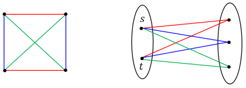
So, 2-register incremental DPs cannot compute (even with unlimited runtime), for example, minimum weight 2-matching of (i.e., complete graph on four vertices), or minimum weight shortest path of (i.e., complete bipartite graph with parts of sizes two and three) from one vertex of the two-sized part to its other vertex ; see Figure 1.
This impossibility is proved using a cut-and-paste argument that is similar to some lower bounds for monotone arithmetic circuit models. We analyze how the paths producing the required monomials intersect with each other; at an intersection point, their sub-paths are patched together to identify a new path which produces a problematic monomial. For monotone arithmetic circuits, the problematic monomial can be any monomial that does not divide any monomial in the polynomial since the model does not allow cancellations. However, this is not sufficient for semirings as monomials can be cancelled by absorption (e.g., over , over both and ). Over these semirings, to prove that a monomial is problematic, we have to show that the value of the monomial is less than the polynomial’s value for some substitution of the variables by constants. Indeed, this is what we do in our impossibility proof. This polynomial has also been used to prove impossibility results for restricted width- ABPs over fields [21].
In contrast, we show that 3-register incremental DPs can compute any polynomial. We prove the more general result:
Theorem 4 (Low Depth Formulas to low Width ABPs).
For any , consider any depth alternating formula of size over or . Then, there is a width ABP of size that simulates the formula .
Note that all polynomials are computable by formulas of depth . By substituting in the above theorem, we conclude that width- ABPs can compute any polynomial. In particular, minimum weight 2-matching of and minimum weight shortest -to- path of have poly-size width- ABPs because the corresponding polynomials are sparse (i.e., have polynomial-sized formulas). This illustrates a stark contrast between power of -register and -register incremental DPs.
Interpreted for arbitrary , the above results shows that any memoization-free alternating DP algorithm that is highly parallelized (i.e., consists of only a few update rounds) can be efficiently simulated using an incremental DP algorithm that updates only a few table entries per round.
Combined with a known DP algorithm for Shortest Path problem based on merging equal-length subpaths, Theorem 4 gives the following corollary (see details in Section 5):
Corollary 5 (Width-reduction for ABPs).
Any ABP of size over or can be converted into an equivalent width ABP of size for any . So, in particular, any ABP over or can be converted into an equivalent logarithmic width ABP with a quasi-polynomial blow-up in its size.
In Section 6, we show that despite their non-universality, 2-register incremental DP algorithms can at least compute all - bivariate polynomials (i.e., every monomial has coefficient or ) over efficiently. The proof of this result crucially relies on absorption properties of semirings.
Theorem 6 (Width-2 ABPs for - Bivariate polynomials over ).
Any - bivariate polynomial over is computable by a size width-2 ABP.
1.7 Proof Outlines
In Section 4, we show that width-2 ABPs cannot compute over and . A high level description of this proof is as follows: First, we show that any ABP computing the above polynomial must have three paths, one for each monomial, such that each of these three paths contains both variables of the corresponding monomial exactly once each and no variable from the other two monomials. Then, we traverse the ABP from left-to-right and mark a layer based on the first variable occurrence amongst the edges of these three paths. Next, we traverse further to mark another layer based on the first variable occurrence amongst the edges of the remaining two paths. At this marked layer, we analyze the possible orientations of edges from the three paths entering into and exiting from it. For each possibility, we show a way to patch sub-paths from two of the three paths to form a new path; further, we analyze the possible weights of this new path and for each possibility, we show that the weight of this new path takes a value strictly lesser than the value taken by for some choice of variable substitution, which is a contradiction. We make this argument precise in the proof of Theorem 3.
In Section 5, we show how to simulate any size depth alternating formula using a width ABP of size over and . A high-level description of this proof is as follows: We associate a carefully chosen format matrix with each of the levels of the formula. Moving bottom-to-top, we describe how to obtain width ABPs that computes the outputs of nodes in any level (in format associated with level ) using the width ABPs already built to compute outputs of nodes in level (in format associated with level ). We make this construction precise in the proof of Theorem 4.
In Section 6, we show that despite their non-universality, width-2 ABPs can at least compute all - (i.e., all monomials have coefficients or ) bivariate polynomials over . A high level description of this proof is as follows: If a monomial has both a higher power and a higher power than another monomial, then the former monomial always (i.e., for any possible variable subsitution) takes larger values than (and so, can be safely absorbed into) the latter monomial. After such absorptions, the monomials that remain are such that the higher their powers, the lower their powers. We construct a width-2 ABP that has all ’s along the top level and all ’s along the bottom level. The two levels are joined by suitably placed bridges. Any source-to-sink path first covers up some region of the bottom level, takes a bridge to jump to the top level, and then covers up some region of the top level. The earlier it takes the bridge jump, the lower its weight’s power and higher its weight’s power. Similarly, the later it takes the bridge jump, the higher its weight’s power and lower its weight’s power. This enables us to have a path for each monomial. We make this construction idea precise in the proof of Theorem 6.
2 Preliminaries
Let be a set equipped with addition (denoted as ) and multiplication (denoted as ) operations. Then, is called a semiring if i) is a commutative monoid, ii) is a monoid, iii) multiplying (from either side) the additive identity with any element of gives back the additive identity, and iv) multiplication (from either side) distributes over addition. Based on the definition of monoid, the first and second conditions together can be alternatively put as follows: i) is closed under and , ii) both and are associative, iii) is commutative, and iv) there exist additive and multiplicative identities. Semirings generalize rings (which, in turn, generalize fields by allowing elements to not have multiplicative inverses) by allowing elements to not have additive inverses.
Min-plus semirings and .
We use and to denote the semirings and respectively, where is the set of all real numbers, is the set of all non-negative real numbers, denotes the minimum operation (which serves as the semirings’ addition operation), and denotes usual addition (which serves as the semirings’ multiplication operation). The multiplicative and additive identities of and are and respectively. Note that and are idempotent, i.e., for all (or ). For any variable and any integer , we use to denote .
Polynomials over and .
An -variate polynomial over min-plus semiring ( or ) is of the form (where the coefficients ’s are elements of , and only finitely many of them are ), which naturally defines a function from to as follows: For every , the corresponding function maps to , i.e., polynomial ’s value upon substituting variables as respectively. For any two polynomials and over , if the value taken by is always (i.e., for each possible substitution of the variables from ) at least the value taken by , then defines the same function as . So, can be absorbed into , i.e., we shall treat and as same. For example, over (but not ), and over both and . This is because for all , and for all (or ). Also, if two polynomials and over define the same function from to , we shall treat them as equivalent to each other with respect to computation; that is, if a computational model (e.g., formula, circuit, ABP) computes , then we shall also say that it computes , and vice versa.
It may be worth noting that the above examples can be generalized to get the following identities: i) For any polynomials and over , we have , and ii) for any polynomials over (or ) and any integer , we have . In the second identity, any other term (where ) in multinomial expansion of LHS gets absorbed into . So, for instance, degree complete homogeneous symmetric polynomial, degree power sum symmetric polynomial and power of degree 1 elementary/complete homogeneous symmetric polynomial over (or ) define the same function.
Due to space limitations, we omit adding more preliminaries here; see full version [15] of this paper for preliminaries related to -families and -projections, ABPs and their weak, weakest & general models, and permanent & Hamiltonian cycle families over min-plus semirings.
It may be worth noting that as described in [5], any univariate polynomial over can be written as a product of linear factors based on its tropical roots/break points, i.e., points at which slope of the univariate polynomial (viewed as a function) changes; equivalently, these are the points where the minimum is attained by at least two monomials. See Figure 12 in full version [15] of this paper for an example. So, any univariate polynomial over can be computed using a weak/general width- ABP. Also, any univariate polynomial can be computed by a weakest width-2 ABP (see Figure 13 in full version [15] of this paper). In this paper, we mostly work with weakest ABPs (except in Section 3.4, which considers general ABPs).
3 and its Analogue over and
Recall that over any field , the class consists of all -families expressible as a hypercube sum over a family in using polynomially-many hypercube variables which take Boolean values and . Note that the additive and multiplicative identities of and are and respectively. So, an obvious attempt to define over and would be to keep the same definition except that the hypercube variables take Boolean values and (instead of and ). That is, would consist of all -families for which there exists a -family and polynomials & such that , where are hypercube variables. Now, view as a polynomial in whose coefficients are polynomials in . That is, is of the form for some polynomials ’s in . Plugging this ’s expression in ’s expression,
Changing the order of the two summations (i.e., actually, two minimums), we get
which has polynomial-sized circuit; so, this definition of makes it coincide with .
3.1 Allowing Complements of Hypercube variables
Over any field , suppose that we modify the definition of to say that the hypercube sum’s summand is allowed to be a polynomial in the complements of hypercube variables (apart from the original variables and hypercube variables), where the complement of any hypercube variable takes values and when takes values and respectively. However, since for any hypercube variable , this modified definition of is same as its original definition. Now, let us mimic this modification over and as follows: Define to consist of those -families for which there exists a -family and polynomials & such that , where the complement of any hypercube variable takes values and when takes values and respectively. Unlike fields (where ), cannot be realized as a polynomial expression in over and . So, it is conceivable that this modified definition may strictly strengthen the obvious definition of attempted above (i.e., separate it from ). To show that this is indeed true, we prove that the permanent family (which needs sized circuits over and [9] and so, ) satisfies this definition as follows: Recall that . Note that every map from to can be specified by a - matrix of size , where for every , its row indicates binary encoding of ’s image under . Also, all permutations (i.e., bijective maps) correspond to those such matrices wherein all rows are distinct. So, we write
where for every , denotes the binary encoding of , and denotes the indicator function (i.e., it takes values and when the statement enclosed within is true and false respectively). Thus, we get the following expression for :
3.2 Spectrum of number of Complementable Hypercube variables – A Dichotomy Theorem
While our first attempt to define allowed no hypercube variable to be complemented, the modified definition above allowed all the polynomially-many hypercube variables to be complemented. Between these two extremes, lies a spectrum of definitions based on how many hypercube variables are allowed to be complemented. For any function , let denote the class corresponding to the definition that allows many hypercube variables to be complemented. We analyze how the relationship between and changes as is varied. In particular, we show the following dichotomy theorem.
Theorem 1.
[Restated, see original statement.]
For semirings or , when , and when , where denotes the number of hypercube variables allowed to be complemented in the definition of .
First, we show that when as follows: Consider the family defined as , where denotes the function for which . As described earlier, can be written as a hypercube sum using hypercube variables and their complements. Also, needs sized circuits over and [9]. Therefore, , as desired.
Next, we show that when as follows: Consider any family . Then, there exists a family and polynomials & such that . Now, view as a polynomial in whose coefficients are polynomials in . That is, is of the following form:
for some polynomials ’s in . Also, any summand wherein some hypercube variable and its complement both have a positive power vanishes. That is, if both and are for some , then the summand evaluates to . This is because for such a summand, when , and when . So, all such summands can be safely dropped. So, we are left with only those summands wherein for each , only one of and appears. Thus, we can express in the following form:
for some polynomials ’s in , and where for each , when , and when . Next, plugging the above expression of in the expression of , and then changing the order of the two summations (i.e., actually, two minimums), we get the following expression for :
Note that because the summand corresponding to for all and for all is ; here, for each , is defined as 0 when not-comp, and when comp. So, we get
| (1) |
For every , let denote the polynomial obtained from by substituting as for all and as for all . Then, note that
| (2) |
Therefore, using (1) and (2), we get . So, as has an sized circuit for each , it follows that can be computed by a circuit of size . Thus, we have , as desired.
3.3 via Hypercube sum over Width-2 ABPs
The proof of (and so, ) over fields in [18] works almost as is over and too (explained in Appendix A.5 in full version [15] of this paper). For any -family , this proof converts circuit computing into an equivalent polynomial-sized multiplicatively disjoint circuit , expresses as the sum of values of parse trees of , and then re-expresses this sum in terms of indicator variables (which serve as hypercube variables) to go over all subgraphs of , using certain indicators to ensure that only the summands corresponding to parse trees survive. This gives
where , are hypercube variables,
Let (respectively ) be the left child (resp. right child) of in the circuit .
As ’s, ’s, ’s, ’s and ’s have polynomial-sized formulas, so does . In full version [15] of this paper, we show that each of these also has a polynomial-sized width-2 ABP. Then, concatenating (to get the product of) all these polynomially-many width-2 ABPs would give a polynomial-sized width-2 ABP that computes , thereby strengthening to , where consists of families expressible as hypercube sum over a family with polynomial-sized width-2 ABPs over (or ).
3.4 via Hypercube sum over general Width-1 ABPs
Over , we show that each of ’s, ’s, ’s, ’s and ’s (as in the previous subsection) are also expressible as hypercube sum over product of constant many linear forms; due to space limitations here, we present this proof in full version [15] of this paper. Then, multiplying all these expressions together would give a way to express (and so, also ) as a hypercube sum over product of polynomially-many linear forms, thereby strengthening to , where consists of families expressible as hypercube sum over a family with polynomial-sized width-1 general (i.e., edge labels can be linear forms) ABPs over .
3.5 Hamiltionian Cycle family in
In full version [15] of this paper, we show that the Hamiltonian cycle family belongs to ; due to space limitations, we omit this proof here.
In 2015, Grochow proved that over any totally ordered semiring, Hamiltonian cycle family cannot be obtained as a monotone affine -projection of the permanent family (see Theorem 4.2 in [7]). So, in particular, , cannot be obtained as a -projection of over . Therefore, since , it follows that is not hard under -projections.
4 Non-Universality of Width-2 ABPs over and
Theorem 3 (Non-universality of Width-2 ABPs).
[Restated, see original statement.]
No width- ABP can compute over and .
Proof.
For the sake of contradiction, assume that there is a width- ABP that computes over (or ). Assume that no edge of is labelled . This is safe because any source-to-sink path containing an edge labelled contributes nothing (i.e., contributes , which is the additive identity) to the sum of weights of all source-to-sink paths. First, we show the following lemma; due to space limitations here, its proof is presented in full version [15] of this paper.
Lemma 1.
For each , there is a source-to-sink path in that has exactly one , exactly one and none of the other four variables (proved for below, and similar argument holds for and too).
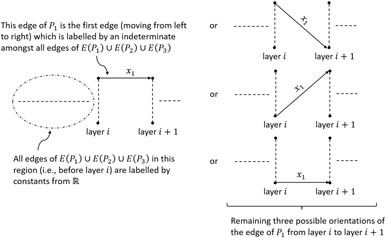
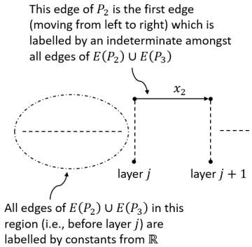
Amongst the edges that appear in , consider a first (moving from left to right) edge that is labelled by an indeterminate. Without loss of generality, assume that this edge belongs to path , and it is labelled by . Also, let and denote the indices of the layers containing the tail and head of this edge respectively. This edge has four possible orientations, i.e., top level of layer to top level of layer , top level of layer to bottom level of layer , bottom level of layer to top level of layer , and bottom level of layer to bottom level of layer (see Figure 2). Next, amongst the edges that appear in after layer , consider a first (again, moving from left to right) edge that is labelled by an indeterminate. Without loss of generality, assume that this edge belongs to path , and it is labelled by . Also, let and denote the indices of the layers containing the tail and head of this edge respectively. Assume that this edge is directed from top level of layer to top level of layer (see Figure 3); the cases corresponding to the other three orientations of this edge can be analyzed in a similar way.
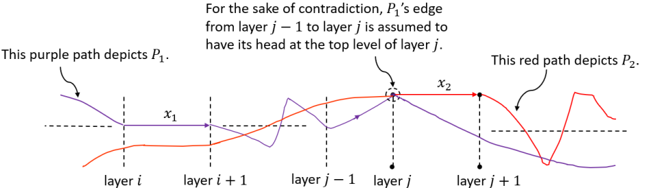
Consider the following two cases: 1) and 2) . We present the proof for Case 1 now, and we present the proof of Case 2 in Appendix A.4 in full version [15] of this paper; its analysis is similar to that of Case 1. First, we show that the edge of from layer to layer must have its head at the bottom level of layer . Suppose not. That is, assume that ’s edge from layer to layer has its head at top level (see Figure 4). Then, ’s portion from layers has no variable, and ’s portion from layers has either zero or one . So, concatenating ’s portion from layers with ’s portion from layers gives a source-to-sink path in whose weight is of the form or for some (or ). We derive a contradiction in both cases as follows: In the former case, . Substituting and gives . In the latter case, . Substituting and gives . This proves that the edge of from layer to layer has its head at bottom level of layer .
Next, consider the edge of from layer to layer . Its tail is same as the head of the edge of from layer to layer (which, as argued above, is at the bottom level of layer ). We show that the head of this edge must be at the bottom level of layer . Suppose not. That is, assume that the edge of from layer to layer is directed from bottom level to top level (see Figure 5). Then, ’s portion from layers has one , and ’s portion from layers has either zero or one . So, concatenating ’s portion from layers with ’s portion from layers gives a source-to-sink path in whose weight is of the form or for some (or ). We derive a contradiction in both cases as follows: In the former case, . Substituting and gives . In the latter case, . Substituting and gives . This proves that the edge of from layer to layer has its head at bottom level of layer .
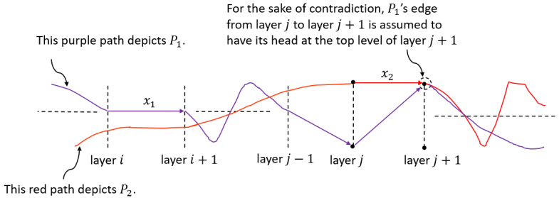
Now, consider the edge of from layer to layer . This edge must be different from the edge joining the top level of layer to the top level of layer ; this is because the latter edge is labelled with , which does not belong to . Also, we show that this edge cannot be directed from bottom level of layer to top level of layer . Suppose not (see Figure 6). Then, ’s portion from layers has one , and ’s portion from layers has no variables or one or one . So, concatenating ’s portion from layers with ’s portion from layers gives a source-to-sink path in whose weight is of the form or or for some (or ). We derive a contradiction in these three cases as follows: In the first case, . Substituting and gives . In the second case, . Substituting and gives . In the third case, . Substituting and gives .
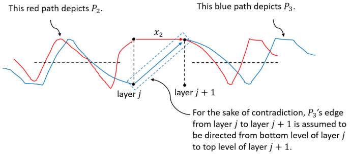
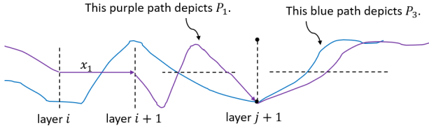
Thus, the edge of from layer to layer has its head at the bottom level of layer . Also, as proved earlier, the edge of from layer to layer has its head at the bottom level of layer . Now, see Figure 7. Note that ’s portion from layers has zero or one . Also, ’s portion from layers has i) no variables, or ii) one , or iii) one . So, concatenating ’s portion from layers with ’s portion from layers gives a source-to-sink path in whose weight is of the form , , , , or for some (or ). We derive a contradiction in these six cases as follows: In the first case, . Substituting and gives . In the second case, . Substituting and gives . In the third case, . Substituting and gives . In the fourth case, . Substituting and gives . In the fifth case, . Substituting and gives . In the sixth case, . Substituting & gives . This proves Theorem 3.
5 Low Depth Formulas to Low Width ABPs over and
Theorem 4 (Low Depth Formulas to low Width ABPs).
[Restated, see original statement.]
For any , consider any depth alternating formula of size over or . Then, there is a width ABP of size that simulates the formula .
So, in particular, logarithmic depth alternating formulas can be efficiently simulated using logarithmic width ABPs. We present the proof of Theorem 4 below.
Proof.
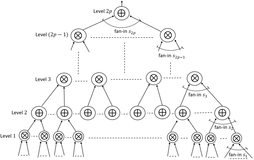
Moving bottom-to-top in the formula , we number the levels as , and let denote the fan-in’s of gates in these levels respectively (see Figure 8). For each , define the format matrix (associated with Level ) as follows222The non- values are highlighted in red for clarity.:
Observe the following format conversions:
-
Using once to get (for any variable/constant ):
-
For every ,
-
–
Using and once each to get :
where first matrix in LHS is obtained by permuting columns of , second matrx in LHS is transpose of , and the matrix in RHS is .
-
–
Using and once each to get :
where first matrix in LHS is , the matrix in RHS is , and second matrix in LHS is obtained from by changing Col1 to ColCol2, scaling Col2 by , permuting columns , and permuting rows ; due to space limitations here, more details about this part are presented in full version [15] of this paper.
-
–
Now, we describe how the above format conversions lead to the desired construction. First, for each Level 1 gate, repeatedly use -to- conversion to get a sequence of matrices that compute its output in format. Next, for each Level 2 gate, repeatedly use -and--to- conversion to get a sequence of matrices that compute its output in format. Next, for each Level 3 gate, repeatedly use -and--to- conversion to get a seqeunce of matrices that computes its output in format. Continuing this process, we finally get a sequence of matrices that compute the output of the top gate (i.e., Level gate) in format. To get ABP size, we put an extra multiplicative factor of as each matrix here has non- entries; so, there are edges between any two layers of the width ABP so constructed. This proves Theorem 4.
It is known that Shortest - Path polynomial over has a depth alternating formula of size (see Section 3.2 in [17]). The corresponding pure DP is as follows: For all vertices and lengths , it stores , i.e., minimum cost of any -to- path that uses edges. To compute ’s, it uses the following recurrence:
where . In the corresponding formula, every (i.e., ) gate has fan-in , every (i.e., ) gate has fan-in and depth of the circuit is . So, the overall formula size is .
This DP works because the optimal path can be obtained by guessing vertices at which the path would be broken if it were to be divided into equal length sub-paths, and then combining optimal paths of lengths each between all pairs of consecutive guessed vertices (computed earlier by the DP). This may be problematic if these optimal paths share common vertices (and so, their merger gives a walk, instead of a path). It is not an issue over (and also, ) because when all costs are non-negative, an optimal path can be recovered from an optimal walk by skipping its portion between first and last appearances of any vertex (i.e., skipping cycles within the walk). Over , we cannot say the same as a skipped cycle may have negative cost (and so, its removal from the walk increases the total cost); nevertheless, we can still use the same DP for acyclic graphs (as then, walks are same as paths) or more generally, graphs containing only non-negative cycles.
Now, as the polynomial computed by any size ABP over or can be seen as a projection of Shortest Path polynomial of a size acyclic graph, we can use the above DP to simulate the ABP by a depth alternating formula of size . Then, using Theorem 4, this formula can be simulated by a width ABP of size . So, we get the following corollary:
Corollary 5 (Width-reduction for ABPs).
[Restated, see original statement.]
Any ABP of size over or can be converted into an equivalent width ABP of size for any . So, in particular, any ABP over or can be converted into an equivalent logarithmic width ABP with a quasi-polynomial blow-up in its size.
6 Width-2 ABPs for - Bivariate Polynomials over
Theorem 6 (Width-2 ABPs for - Bivariate polynomials over ).
[Restated, see original statement.]
Any - bivariate polynomial over is computable by a size width-2 ABP.
Proof.
Let denote the coefficient monomials of , listed in non-increasing order of powers (i.e., ). Suppose that (say ) for some . Then, consider the and monomials, i.e., and respectively. If , then for all possible substitutions of and from and thus, the monomial can be safely dropped (i.e., it gets absorbed into the monomial). Similarly, if , then for all possible substitutions of and from and thus, the monomial can be safely dropped (i.e., it gets absorbed into the monomial). So, after exhaustively making such absorptions, we safely assume that . Next, let us analyze the relative order of magnitudes of powers. Suppose that for some . Then, consider the and monomials, i.e., and respectively. Since and , for all possible substitutions of and from and thus, the monomial can be safely dropped (i.e., it gets absorbed into the monomial). So, after exhaustively making such absorptions, we safely assume that . Due to space limitations here, we present the remaining proof in full version [15] of this paper.
7 Conclusion and Open Problems
As mentioned earlier, the key question that motivated us to begin this work (but is still unresolved) is whether there is an analogue of Ben-Or & Cleve’s result [4] over min-plus semirings and . That is, can formulas be efficiently simulated using bounded-width ABPs over and ? Jukna observed that the sub-semiring is isomorphic to the Boolean semiring via the isomorphism and (see, for example, Lemma 7 in [10]). Using his observation, it can be argued that an analogue of Ben-or & Cleve’s result over min-plus semirings would imply that polynomial-sized monotone Boolean formulas can be simulated using polynomial-sized monotone bounded-width branching programs, i.e., -- thus refuting a conjecture of Grigni and Sipser [6], that function (which is known to belong to -) does not belong to -.
Another direction could be to build upon lower bound proof devised by Jukna and Schnitger in 2016 [12]. They showed that any ABP computing a polynomial (over or ) must have at least as many disjoint cuts333Subset of variable labelled edges that intersects every source-to-sink path. as the length444Smallest monomial degree in any polynomial defining the same function as . of ; so, as size of each cut is at least the cover number555Smallest number of variables which when substituted as make evaluate to . of , the ABP’s size must be at least the product of length and cover number. Their proof works even for unbounded-width ABPs, but it gives only polynomial lower bounds. Strengthening their argument in the context of bounded-width ABPs to get stronger lower bounds is an interesting open problem.
Next, although we defined an analogue of the class over and , it remains to identify -families complete for the class (if any) under -projections. As discussed earlier, permanent family cannot be complete due to [7]; but, is it -complete? Another potential candidate polynomial for over and is the Hamiltonian cycle family .
Also, our arguments for non-universality for width-2 ABPs (Theorem 3) works only for weakest width-2 ABPs. It would be interesting to generalize it to even more general width-2 ABPs. Further, while we showed , it is unclear if this hold true over as well. If yes, it would subsume the result that as weakest width-2 ABPs can efficiently simulate general width- ABPs over . This is because for any constant and variable , can be computed by scaling first row and second column of by and its multiplicative inverse (i.e., ) respectively, where the format matrix supports addition via .
References
- [1] Richard Bellman. On a routing problem. Quarterly of applied mathematics, 16(1):87–90, 1958.
- [2] Richard P Brent. The parallel evaluation of general arithmetic expressions. Journal of the ACM (JACM), 21(2):201–206, 1974. doi:10.1145/321812.321815.
- [3] Karl Bringmann, Christian Ikenmeyer, and Jeroen Zuiddam. On algebraic branching programs of small width. Journal of the ACM (JACM), 65(5):1–29, 2018. doi:10.1145/3209663.
- [4] Richard Cleve. Computing algebraic formulas with a constant number of registers. In Proceedings of the twentieth annual ACM symposium on Theory of computing, pages 254–257, 1988.
- [5] Shelby Cox. Notes on tropical language and applications. https://websites.umich.edu/˜spcox/notes_1.pdf.
- [6] Michelangelo Grigni and Michael Sipser. Monotone complexity. In Proceedings of the London Mathematical Society Symposium on Boolean Function Complexity, pages 57–75, 1992.
- [7] Joshua A Grochow. Monotone projection lower bounds from extended formulation lower bounds. Theory of Computing, 13(18):1–15, 2017. doi:10.4086/TOC.2017.V013A018.
- [8] M Harshil. Diverse Solutions, Modifying Graph Eigenvalues and Bounded-Width ABPs. PhD thesis, Indian Institute of Technology Gandhinagar, 2025.
- [9] Mark Jerrum and Marc Snir. Some exact complexity results for straight-line computations over semirings. Journal of the ACM (JACM), 29(3):874–897, 1982. doi:10.1145/322326.322341.
- [10] Stasys Jukna. Lower bounds for tropical circuits and dynamic programs. Theory of Computing Systems, 57(1):160–194, 2015. doi:10.1007/S00224-014-9574-4.
- [11] Stasys Jukna. Incremental versus non-incremental dynamic programming. Oper. Res. Lett., 46(3):278–281, 2018. doi:10.1016/J.ORL.2018.02.003.
- [12] Stasys Jukna and Georg Schnitger. On the optimality of Bellman–Ford–Moore shortest path algorithm. Theoretical Computer Science, 628:101–109, 2016. doi:10.1016/J.TCS.2016.03.014.
- [13] Kacper Kluk and Jesper Nederlof. Lower bounds on pure dynamic programming for connectivity problems on graphs of bounded path-width. arXiv preprint arXiv:2512.23121, 2025. doi:10.48550/arXiv.2512.23121.
- [14] Vladimir Kolmogorov. Blossom V: a new implementation of a minimum cost perfect matching algorithm. Mathematical Programming Computation, 1(1):43–67, 2009. doi:10.1007/S12532-009-0002-8.
- [15] Balagopal Komarath, Harshil Mittal, and Jayalal Sarma. Vp, vnp and algebraic branching programs over min-plus semirings, 2026. arXiv:2605.09551.
- [16] Joseph B Kruskal. On the shortest spanning subtree of a graph and the traveling salesman problem. Proceedings of the American Mathematical society, 7(1):48–50, 1956.
- [17] Meena Mahajan, Prajakta Nimbhorkar, and Anuj Tawari. Shortest path length with bounded-alternation (min,+) formulas. International Journal of Advances in Engineering Sciences and Applied Mathematics, 11(1):68–74, 2019.
- [18] Guillaume Malod and Natacha Portier. Characterizing Valiant’s algebraic complexity classes. Journal of complexity, 24(1):16–38, 2008. doi:10.1016/J.JCO.2006.09.006.
- [19] Jaroslav Nešetřil, Eva Milková, and Helena Nešetřilová. Otakar boruvka on minimum spanning tree problem translation of both the 1926 papers, comments, history. Discrete mathematics, 233(1-3):3–36, 2001. doi:10.1016/S0012-365X(00)00224-7.
- [20] Robert Clay Prim. Shortest connection networks and some generalizations. The Bell System Technical Journal, 36(6):1389–1401, 1957.
- [21] Chandan Saha, Ramprasad Saptharishi, and Nitin Saxena. The power of depth 2 circuits over algebras. In Ravi Kannan and K. Narayan Kumar, editors, IARCS Annual Conference on Foundations of Software Technology and Theoretical Computer Science, FSTTCS 2009, December 15-17, 2009, IIT Kanpur, India, volume 4 of LIPIcs, pages 371–382. Schloss Dagstuhl – Leibniz-Zentrum für Informatik, 2009. doi:10.4230/LIPIcs.FSTTCS.2009.2333.
- [22] Leslie G Valiant. Completeness classes in algebra. In Proceedings of the eleventh annual ACM symposium on Theory of computing, pages 249–261, 1979. doi:10.1145/800135.804419.
- [23] LG Valiant, S Skyum, S Berkowitz, and C Rackoff. Fast parallel computation of polynomials using few processors. SIAM Journal on Computing, 12(4):641, 1983.
- [24] Heribert Vollmer. Arithmetic Circuits, pages 173–214. Springer Berlin Heidelberg, Berlin, Heidelberg, 1999.